Continuous and discontinuous phase transitions and partial synchronization in stochastic three-state oscillators

Abstract

We investigate both continuous (second-order) and discontinuous (first-order) transitions to macroscopic synchronization within a single class of discrete, stochastic (globally) phase-coupled oscillators. We provide analytical and numerical evidence that the continuity of the transition depends on the coupling coefficients and, in some nonuniform populations, on the degree of quenched disorder. Hence, in a relatively simple setting this class of models exhibits the qualitative behaviors characteristic of a variety of considerably more complicated models. In addition, we study the microscopic basis of synchronization above threshold and detail the counterintuitive subtleties relating measurements of time averaged frequencies and mean field oscillations. Most notably, we observe a state of suprathreshold partial synchronization in which time-averaged frequency measurements from individual oscillators do not correspond to the frequency of macroscopic oscillations observed in the population.

I Introduction

A great number of physical systems consist of individual entities with periodic, or nearly periodic, dynamics. Ranging from collections of chemical consitutents to groups of social entities – for example, applauding individuals whose clapping is repetitive – these systems serve as a battleground of sorts for the competition between the dynamics of individual constituents and the large scale cooperation favored in many cases by the nature of their mutual interactions. Owing to the ubiquity and certainly, in part, to the dramatic nature of the emergent synchronized behavior in such naturally oscillating settings, the subject has been intensely studied in the physics literature for several decades, with the Kuramoto oscillator and its kin serving as prototypical models on which many studies are based strogatz ; winfree ; kuramoto ; strogatz2 .

Recently, a simple class of models of macroscopic synchronization have provided a number of additional insights into the large-scale phenomena ocurring in noisy discrete coupled oscillators, including detailed characterizations of both the universal critical behavior of the continous phase transition threestate1 ; threestate2 as well as the effects of spatial disorder in such populations threestate3 . While retaining many qualitative characteristics of more complex models, the discrete oscillators remain sufficiently simple to provide results unattainable in most of the paradigmatic settings.

In this paper, we generalize our class of stochastic, discrete oscillator models and detail its use in a variety of new contexts. By generalizing the form of the inter-oscillator coupling, we show that our class of mean field models encompasses oscillators which can undergo either supercritical or subcritical Hopf bifurcations, depending on the microscopic specifics of the coupling. In addition, we study dichotomously disordered populations of oscillators and show that the bifurcation can be either supercritical or subcritical depending on the degree of disorder in the population. Such behaviors are reminiscent of a number of significantly more complex oscillator models gianuzzi07 ; filatrella07 ; tanaka ; acebron ; choi ; pazo ; hong0 , including Daido’s generalized Kuramoto oscillators daido , where either disoder or microscopic coupling specifics can alter the nature (continuous or discontinuous) of the transition. However, our model provides a far simpler setting for observing both continous and discontinous transitions to synchronization.

In addition, we study the microscopic underpinnings of synchronization above threshold. In particular, we look at time-averaged frequency and its relationship to phase synchronization above threshold (which turns out to be interestingly counterintuitive). Again, we do this for a specific model from our general class (for both single and dichotomously disordered populations), but we expect the results to hold for our entire class of models undergoing a Hopf bifurcation. This is somewhat similar to the partial synchronization seen in other models rosenblum07 , but again, our model is simpler and, perhaps, more transparent.

In Sec. II we present our model and highlight its essential parameters. Here we note that for systems of oscillators with identical transition rates between states the control parameter for the phase transition is the coupling strength among oscillators; when the array includes oscillators with different transition rates, the degree of disorder is also a control parameter. In Sec. III we show that depending on the values of microscopic parameters, this model can exhibit both subcritical (or first-order) and supercritical (or second-order) phase transitions, as a function of the coupling strength and also as a function of the degree of disorder. Section IV deals with the microscopic underpinnings of the synchronization phenomenon and the connection between phase synchronization and frequency entrainment in our system. Section V presents a summary and further discussion of our results.

II The Model

In this section we present our model in some detail, repeating some of our early presentations threestate1 ; threestate2 ; threestate3 because of important (albeit simple) generalizations of the model. We begin by considering a stochastic three-state model governed by transition rates $g$ (see Fig. 1), where each state may be interpreted as a discrete phase threestate1 ; threestate2 ; threestate3 . Because the transitions among states are unidirectional and do not conform to deterministic rate laws, the model retains a qualitative link with a noisy phase oscillator.

Figure 1: Three-state unit with transition rates $g$.

The linear evolution equation of a single oscillator is $\partial\bm{P}(t)/\partial t=M\bm{P}(t)$, where the components $P_{i}(t)$ of the column vector $P(t)=(P_{1}(t)~{}P_{2}(t)~{}P_{3}(t))^{T}$ ($T$ denotes the transpose) are the probabilities of being in states $i$ at time $t$, where $i=1,2,3$ and

$$M=\begin{pmatrix}-g&0&g\\ g&-g&0\\ 0&g&-g\end{pmatrix}.$$ (1)

The system reaches a steady state for $P_{1}^{*}=P_{2}^{*}=P_{3}^{*}=1/3$. The oscillator’s periodicity, as contained in the timescale of the cycle $i=1\rightarrow 2\rightarrow 3\rightarrow 1...$, is determined by $g$; that is, the time evolution of our simple model qualitatively resembles that of the discretized phase of a generic noisy oscillator with the intrinsic eigenfrequency set by the value of $g$.

To study interacting arrays of these oscillators, we couple individual units by allowing the transition rates of each unit to depend on the states of the units to which it is connected. Specifically, for $N$ identical units we choose the transition rate of a unit $\nu$ from state $i$ to state $i+1$ as

$$g_{i}=g\exp\left[{\frac{a(UN_{i+1}+VN_{i-1}+WN_{i})}{n}}\right],$$ (2)

where $i=1,2,3$ and $i+1=1$ when $i=3$, $a$ is the coupling parameter, $g$ is the transition rate parameter, $n$ is the number of oscillators to which unit $\nu$ is coupled, and $N_{k}$ is the number of units among the $n$ that are in state $k$. We introduce the real constants $U$, $V$, and $W$ to encompass in a general way our two previous coupling functions threestate1 ; threestate2 ; threestate3 . Each unit may thus transition to the state ahead or remain in its current state, and the propensity for such a change depends on the states of its nearest neighbors. In our earlier works we considered the globally coupled system, $n=N-1$, and also nearest neighbor coupling in square, cubic, or hypercubic arrays, $n=2d$ ($d=$ dimensionality). Here we focus on globally coupled arrays.

For a population of $N\to\infty$ identical units in the mean field (globally coupled) version of this model we can replace $N_{k}/N$ with the probability $P_{k}$, thereby arriving at a nonlinear equation for the mean field probability, $\partial\bm{P}(t)/\partial t=M[\bm{P}(t)]\bm{P}(t)$, with

$$M[\bm{P}(t)]=\begin{pmatrix}-g_{1}&0&g_{3}\\ g_{1}&-g_{2}&0\\ 0&g_{2}&-g_{3}\end{pmatrix}.$$ (3)

Normalization allows us to eliminate $P_{3}(t)$ and obtain a closed set of equations for $P_{1}(t)$ and $P_{2}(t)$. We can then linearize about the fixed point $(P_{1}^{*},P_{2}^{*})=(1/3,1/3)$, yielding a Jacobian $A(a,g,U,V,W)$ with a set of complex conjugate eigenvalues which determine the stability of this asynchronous state. Specifically, we find that

$$\lambda_{\pm} =C\big{(}-9+3a\Delta_{UW}$$ (4)

$$\pm i\sqrt{3}(3+a(U+W-2V))\big{)},$$

where $C\equiv ge^{a(U+V+W)/3}/6$ is a nonzero constant for all finite $U$, $V$, and $W$ and we introduce the abbreviation $\Delta_{mn}\equiv m-n$. The eigenvalues cross the imaginary axis at $a_{c}=3/\Delta_{UW}$, yielding

$$\lambda_{\pm}^{*}=\pm i\omega(U,V,W)$$ (5)

with

$$\omega(U,V,W)\equiv g\sqrt{3}e^{a(U+V+W)/\Delta_{UW}}\frac{\Delta_{UV}}{\Delta_{UW}}.$$ (6)

For $\Delta_{UW}\neq 0$ and $\omega(U,V,W)\neq 0$ (that is, $\Delta_{UV}\neq 0$), $a_{c}$ represents a Hopf bifurcation point, indicating the emergence of macroscopic oscillations indicative of synchronization. Furthermore, we require that $\Delta_{UW}>0$ to ensure the bifurcation happens at a positive value of $a$. We note that in previous studies we have used $(U,V,W)=(1,-1,0)$, yielding $a_{c}=3$ and $\omega=2g\sqrt{3}$ threestate3 , and $(U,V,W)=(1,0,-1)$, yielding $a_{c}=1.5$ and $\omega=g\sqrt{3}/2$ threestate1 ; threestate2 . In addition, we stress that while a range of models may prove useful for exploring the phase transition behavior near threshold (see, for example, threestate1 ; threestate2 ), only models with $W=0$ provide physically appealing characteristics far above threshold (see, for example, threestate3 ). Specifically, only for $W=0$ does the frequency of a perfectly synchronized set of oscillators maintain a nonzero finite value ($g$). Below we explore in more detail the nature of the Hopf bifurcation associated with the class of models described by the permitted values $(U,V,W)$.

Figure 2: (Color online) In a single population of globally coupled oscillators, two physically distinct Hopf transitions can be observed depending on the choices of $U$, $V$, and $W$. The top panel represents $(U,V,W)=(1,-2,0)$ and clearly shows characteristics of a continous transition, including hysteresis. Squares represent solutions starting from ordered (mostly synchronized) initial conditions, while circles represent solutions starting from disordered (random) initial conditions. The bottom panel represents $(U,V,W)=(2,-1,0)$ and displays a continous transition with critical exponent $\beta$ given by the classical value 1/2. The inset shows a log-log plot near the critical point. For comparison, a dashed line with a slope of 1/2 is shown along with the order parameter curve (solid line) to verify this scaling relation.

In addition to the single population case, we consider globally coupled arrays of oscillators that can have one of $\mathcal{N}\leq N$ different transition rate parameters, $g=\gamma_{u}$, $u=1,\ldots,\mathcal{N}$. As detailed in threestate3 , the probability vector is now $3\mathcal{N}$-dimensional, $\bm{P}(t)=(P_{1,\gamma_{1}}~{}P_{2,\gamma_{1}}~{}P_{3,\gamma_{1}}~{}\cdots~{}P_{1,\gamma_{\mathcal{N}}}~{}P_{2,\gamma_{\mathcal{N}}}~{}P_{3,\gamma_{\mathcal{N}}})^{T}$, and the added subscript on the components of $\bm{P}(t)$ keeps track of the transition rate parameter. Explicitly, the component $P_{i,\gamma_{u}}$ is the probability that a unit with transition rate parameter $g=\gamma_{u}$ is in state $i$. The evolution of the probability vector is given by the set of coupled nonlinear differential equations $\partial\bm{P}(t)/\partial t=M_{\mathcal{N}}[\bm{P}(t)]\bm{P}(t)$, with

$$M_{\mathcal{N}}[\bm{P}(t)]=\begin{pmatrix}\mathcal{M}_{\gamma_{1}}&0&\ldots&0\\ 0&\mathcal{M}_{\gamma_{2}}&\ldots&0\\ :&:&:&:\\ 0&\ldots&0&\mathcal{M}_{\gamma_{\mathcal{N}}}\end{pmatrix}.$$ (7)

Here

$$\mathcal{M}_{\gamma_{u}}=\begin{pmatrix}-g_{1}(\gamma_{u})&0&g_{3}(\gamma_{u})\\ g_{1}(\gamma_{u})&-g_{2}(\gamma_{u})&0\\ 0&g_{2}(\gamma_{u})&-g_{3}(\gamma_{u})\end{pmatrix},$$ (8)

and

$$g_{i}(\gamma_{u}) =\gamma_{u}\exp\bigg{[}a\sum_{k=1}^{\mathcal{N}}\varphi(\gamma_{k})$$ (9)

$$\times\left(UP_{i+1,\gamma_{k}}+VP_{i-1,\gamma_{k}}+WP_{i,\gamma_{k}}\right)\bigg{]}.$$

The function $\varphi(\gamma_{k})$ is the fraction of units which have a transition rate parameter $g=\gamma_{k}$.

Because it closely appeals to physical intuition threestate3 for oscillators far above threshold, we limit ourselves to the case $(U,V,W)=(1,-1,0)$ for dichotomously disordered oscillators. We further limit our focus here to uniform distributions $\varphi(\gamma_{k})=1/{\mathcal{N}}$, but note that relaxing this constraint has been shown to preserve the qualitative features of the model threestate3 . For uniform distributions and $(U,V,W)=(1,-1,0)$, probability normalization again allows us to reduce this to a system of $2\mathcal{N}$ coupled ordinary differential equations. We can then linearize about the disordered state $\bm{P}(t)=(1/3~{}1/3~{}\ldots~{}1/3)^{T}$ and arrive at a $2\mathcal{N}\times 2\mathcal{N}$ Jacobian parameterized by a collection of $\mathcal{N}$ transition rate parameters ${\gamma_{i}}$ and a coupling strength $a$.

While it has been shown that the qualitative essence of the model remains similar for $\mathcal{N}=2,3,4$ and even for completely disordered populations threestate3 , we focus here only on the simple dichotomously disordered case, $\mathcal{N}=2$. As shown in threestate3 , the four eigenvalues $(\lambda_{+},\lambda_{+}^{*},\lambda_{-},\lambda_{-}^{*})$ of the corresponding Jacobian are given by

$$\frac{{\rm Re}\lambda_{\pm}}{\gamma_{1}+\gamma_{2}} =\frac{1}{8}\left[a-6\pm\mathcal{B}(a,\mu)\cos\left(\mathcal{C}(a,\mu)\right)\right],$$ (10)

$$\frac{{\rm Im}\lambda_{\pm}}{\gamma_{1}+\gamma_{2}} =\frac{1}{8}\left[\sqrt{3}(a+2)\pm\mathcal{B}(a,\mu)\sin\left(\mathcal{C}(a,\mu)\right)\right],$$

where

$$\mathcal{B}(a,\mu) \equiv\sqrt{2}\left[a^{4}-6a^{2}\mu^{2}+3\mu^{4}(a^{2}+3)\right]^{1/4},$$ (11)

$$\mathcal{C}(a,\mu) \equiv\frac{1}{2}\tan^{-1}\left(\frac{-\sqrt{3}(a^{2}-(a+3)\mu^{2})}{a^{2}+3(a-1)\mu^{2}}\right).$$

and

$$\mu\equiv\frac{2|\gamma_{1}-\gamma_{2}|}{(\gamma_{1}+\gamma_{2})}.$$ (12)

Aside from an overall factor $(\gamma_{1}+\gamma_{2})$, Eqs. (10) depend only on the relative width variable $\mu$, and therefore the critical coupling $a_{c}$, that is, the value of $a$ at which Re $\lambda_{+}=0$, depends only on $\mu$. As Re $\lambda_{-}$ does not vanish for any $a$, $a_{c}$ corresponds to a Hopf bifurcation, and our $\mathcal{N}=2$ model exhibits macroscopic oscillations indicative of large-scale cooperation. We note that $a_{c}$ increases with increasing $\mu$, indicating that a stronger coupling is necessary to overcome increasingly different values of $\gamma_{1}$ and $\gamma_{2}$.

In what follows, we make use of the synchrony order paramter $r$ to characterize the emergence of phase synchrony hong . This parameter is defined as

$$r=\langle R\rangle,\qquad R\equiv\frac{1}{N}\lvert\sum_{j=1}^{N}e^{i\phi_{j}}\rvert.$$ (13)

Here $\phi$ is a discrete phase, taken to be $2\pi(k-1)/3$ for state $k\in\{1,2,3\}$ at site $j$. The brackets represent an average over time in the steady state and an average over all independent trials. Therefore, $r$ serves as a measure of phase synchronization.

III Continuous and Discontinuous Transitions to Synchrony

In the mean field limit, the order of the phase transition to synchrony is closely tied to the nature of the Hopf bifurcation. Specifically, a subcritical Hopf bifurcation corresponds to a discontinuous (sometimes called first-order) phase transition, while a supercritical Hopf bifurcation indicates a continuous (second-order) transition. As such, we place special emphasis in this manuscript on the sign of $l_{1}$, the first Lyapunov coefficient, which provides information on the nature of the Hopf bifurcation and, by extension, on the order of the phase transition.

Figure 3: The first Lyapunov coefficient $l_{1}$ is shown for Hopf bifurcations taking place at $\epsilon^{H}=(a_{c}(\mu),\mu)$. The bifurcation can be either subcritical or supercritical depending on the relative width variable.

In general, $l_{1}$ can be calculated using the projection technique given in kuznetsov , which relies on a multivariate Taylor expansion of the vector field describing the dynamics in question about an equilibrium point. For a general $n$-dimensional dynamical system $\dot{x}=f(x,\epsilon)$ with an equilibrium point $x=x^{H}$ undergoing a Hopf bifurcation at parameter value $\epsilon=\epsilon^{H}$, $l_{1}$ is given by kuznetsov

$$l_{1}=\frac{1}{2\omega} \mbox{Re}(\langle p,C(q,q,\bar{q})\rangle-2\langle p,B(q,A^{-1}B(q,\bar{q}))\rangle$$ (14)

$$+\langle p,B\left(\bar{q},(2i\omega I-A)^{-1}B(q,q)\right)\rangle),$$

where $\langle.,.\rangle$ is the typical complex scalar product, $I$ is the identity matrix, and $p$ and $q$ are right and left eigenvectors of the Jacobian $A=\frac{\partial f}{\partial x}\big{|}_{x=x^{H}}$ given by

$$Aq =i\omega q$$ (15)

$$A^{T}p =-i\omega p.$$

Furthermore, $p$ is chosen so that $\langle p,q\rangle=1$, and $B(u,v)$ and $C(u,v,w)$ are multilinear, $n$-dimensional vector functions corresponding to the lowest order nonlinear coefficients in the Taylor expansion of the vector field. That is,

$$B(u,v) =\sum_{j,k=1}^{n}\frac{\partial^{2}f(\psi,\epsilon^{H})}{\partial\psi_{j}\partial\psi_{k}}\bigg{|}_{\psi=x^{H}}u_{j}v_{k},$$ (16)

$$C(u,v,w) =\sum_{j,k,l=1}^{n}\frac{\partial^{3}f(\psi,\epsilon^{H})}{\partial\psi_{j}\partial\psi_{k}\partial\psi_{l}}\bigg{|}_{\psi=x^{H}}u_{j}v_{k}w_{l},$$

with $x^{H}$ indicating the equilibrium point of the vector field around which we expand and $\epsilon^{H}$ the bifurcation parameter, $\epsilon$, evaluated at the bifurcation point.

Figure 4: (Color online) A subcritical Hopf bifurcation occurs for $\mu=3/4$. Squares represent solutions starting from ordered (mostly synchronized) initial conditions, while circles represent solutions starting from disordered (random) initial conditions. Dark (blue) points correspond to population one, $\gamma_{1}=2.5$, and light (pink) points to population two, $\gamma_{2}=5.5$. The transition is clearly discontinuous as $a$ crosses $a_{c}\approx 3.55$. In addition, a region of multistability and corresponding hysteresis exists just below threshold.

III.1 Continuous and Discontinuous Transitions in a Single Population of Identical Oscillators

For the case of a single population of oscillators described by Eqs. (2) and (3), $l_{1}$ can be analytically calculated using the technique outlined above. Specifically, we set $g=1$ (without loss of generality) and consider the equilibrium point $\bm{P}=(1/3,1/3)$ at $\epsilon^{H}\equiv a_{c}$ and find $q$ and $p$ to be

$$q =\left(-\frac{1}{2}+\frac{i\sqrt{3}}{2},1\right),$$ (17)

$$p =\left(\frac{i-\sqrt{3}}{3i+\sqrt{3}},\frac{2i}{3i+\sqrt{3}}\right),$$

independent of $U$, $V$, and $W$. Then, calculating the multivariable functions $B(u,v)$ and $C(u,v,w)$ with Eq. (16) and using $\omega$ as defined in Eq. (6) along with Eqs. (14) and (17), we find after simplification that

$$l_{1}=-\frac{9\sqrt{3}(U+V-2W)}{4\Delta_{UW}}.$$ (18)

As a result, the nature of the Hopf bifurcation depends on the choices $U$, $V$, and $W$. Specifically, if we assume $U>V$, we have

$$l_{1} <0\mbox{ for }W<\frac{U+V}{2};$$ (19)

$$l_{1} >0\mbox{ for }W>\frac{U+V}{2}.$$

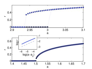
A similar result holds for $U<V$, but we shall here restrict ourselves to the intuitively reasonable models positing $U\geq 0$ and $V\leq 0$; that is, the oscillators one state ahead of the one in question can only increase (or not affect) the transition rate and those behind can only decrease (or not affect) the transition rate. To verify these predictions, we show numerical solutions to the mean field equations in Fig. 2; the top panel represents an example in the subcritical regime ($(U,V,W)=(1,-2,0)$) while the bottom panel shows an example in the supercritical regime ($(U,V,W)=(2,-1,0)$). A clear distinction can be made in the neighborhood of the critical point. We also note that the continuous transition is characterized by the classical mean field exponent $\beta=1/2$.

We further observe that the choice $(U,V,W)=(1,0,-1)$ leads to $l_{1}=-27\sqrt{3}/4\approx-11.69$, indicating a supercritical Hopf bifurcation and rendering the model applicable to studies of continuous phase transitions threestate1 ; threestate2 . With universality in mind, we stress that any choice of parameters $(U,V,W)$ yielding a supercritical bifurcation should show similar critical behavior. On the other hand, the choice $(U,V,W)=(1,-1,0)$, while physically appealing above threshold, falls at a singular point separating the subcritical and supercritical cases ($l_{1}=0$). The flexibility inherent in the choice of coefficients $X$, $Y$, and $Z$ speaks to the richness of our generic three-state oscillator and highlights its utility in studying synchronization in both supercritical (see threestate1 ; threestate2 ) and subcritical regimes. We proceed to study the model in the presence of dichotomous disorder and show that, for a given choice $(U,V,W)$, the level of disorder can also alter the nature of the Hopf bifurcation and hence the order of the phase transition. We select the physically appealing choice $(1,-1,0)$ and, while the behavior near the critical point may depend in some sense on this choice, we stress that our overarching goal remains unhindered. That is, we are able to provide an example indicating that disorder alone can affect the nature of the transition. The ubiquity of this phenomenon across the entire range of models remains an open question for future work, though we note that similar results are observed for all parameter choices mentioned in this paper.

Figure 5: (Color online) A supercritical Hopf bifurcation occurs for $\mu=7/4$. Squares represent solutions starting from an ordered (mostly synchronized) initial condition, while circles represent solutions starting from a disordered (random) initial condition (repetition with other ordered and disordered initial conditions leads to essentially the same results). Dark (blue) points correspond to population one, $\gamma_{1}=0.25$, and light (pink) points to population two, $\gamma_{2}=3.75$. The transition is clearly continuous as $a$ crosses $a_{c}\approx 5.44$, and there is a noticeable absence of hysteresis. Dotted line is drawn to guide the eye. The inset indicates that, in the neighborhood of the critical point, the order parameter follows power law behavior with the correct mean field critical exponent ($\beta=1/2$).

III.2 Continuous and Discontinuous Transitions in a Dichotomously Disordered Population

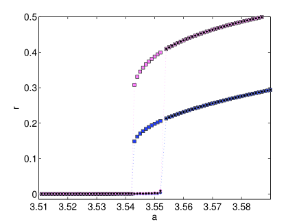
Interestingly, the dichotomously disordered system corresponding to Eqs. (7), (8), and (9) with $\mathcal{N}=2$ and $(U,V,W)=(1,-1,0)$ can undergo either a subcritical or supercritical bifurcation depending on the value of $\mu$ characterizing the individual transition rates. The transition to synchrony occurs at a single value of the coupling $a_{c}(\mu)$ dependent on the relative width parameter threestate3 . As such, $a$ and $\mu$ are not truly independent parameters, and we can in principle eliminate $a$ and consider $\mu$ to be the bifurcation parameter of interest. Then, using the machinery of Eqs. (14), (15), and (16), it is a straightforward but tedious exercise to numerically evaluate the first Lyapunov coefficient $l_{1}(\mu)$ corresponding to the Hopf bifurcation occurring at $(\mu,a(\mu))$. As shown in Fig. 3, the sign of $l_{1}$ varies depending on the relative width parameter (which in turn determines the critical coupling $a_{c}$). Hence, the phase transition to synchrony can appear continuous or discontinuous depending on the relative difference between the transition rate parameters in the two populations.

Figure 6: (Color online) Each plot shows a histogram of time-averaged frequencies (in the steady state), where the vertical axis represents the number of units (out of $N=3500$ total units) having the frequency $\bar{\omega}$. The power spectrum of $P_{1,\gamma_{1}}$ overlays each histogram. The top panel is below synchronization threshold ($a=2.65$), while the middle ($a=3.05$) and lower panels ($a=3.45$) are both above threshold.

To verify these predictions, we solve the mean field equations numerically in both the subcritical ($\mu=3/4$) and supercritical ($\mu=7/4$) regimes. In the former case, we consider the case $\gamma_{1}=2.5$, $\gamma_{2}=5.5$. Figure 4 clearly indicates that the transition to synchrony is marked by a discontinuous change in the order parameter $r$ as $a$ eclipses $a_{c}\approx 3.55$. In addition, a small region of marked hysteresis appears just below threshold. Remarkably, this indicates that a stable disordered solution coexists with a stable, synchronized solution (the stable limit cycle) just before threshold.

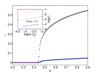
By contrast, the case $\mu=7/4$ corresponds to a supercritical Hopf bifurcation reminiscent of a continuous phase transition. As shown in Fig 5, the transition is characterized by a continously increasing order parameter; no hysteresis is evident. We note also that the order parameter displays a power law increase near the onset of the bifurcation marked by the mean field critical exponent $\beta=1/2$. This is expected both from the Hopf bifurcation theorem, which prescribes the $(a-a_{c})^{1/2}$ dependence of the limit cycle radius (closely related to $r$, the order parameter) near the onset of synchrony, and also because of the analogy with phase transitions in an infinite-dimensional space (see threestate1 ; threestate2 ).

Interestingly, these results indicate that the degree of spatial disorder may fundamentally alter the nature of the phase transition to synchrony. In both the subcritical and supercritical cases, synchronization is marked by the destabilization of the non-synchronous state at a single value of $a_{c}$, giving rise to emergent oscillations in a macroscopic variable [for example, $P_{1,\gamma_{i}}(t)$]. Hence, both cases retain the qualitative features of synchronization in disordered populations discussed in our previous work threestate3 ; however, the details of the onset of such cooperation distinguish the two cases.

Figure 7: (Color online) Each plot shows a histogram of time-averaged frequencies (in the steady state), where the vertical axis represents the number of units (out of $N=3500$ total units) having the frequency $\bar{\omega}$. Population one, characterized by $\gamma_{1}=2.5$, is represented by the dark (blue) histogram, while population two, characterized by $\gamma_{2}=5.5$, is represented by the light (pink) one. Power spectra of $P_{1,\gamma_{1}}$ (dark, blue) and $P_{1,\gamma_{2}}$ (light, pink) overlay the histograms. The top panel is below synchronization threshold ($a=3.20$), while the middle ($a=3.60$) and lower panels ($a=3.86$) are just above threshold. For aesthetic purposes, the horizontal range is relatively shifted in the three panels.

IV Microscopic Underpinnings of Synchronization

Having detailed two distinct mechanisms by which synchronization might arise, we now explore in detail the microscopic subtleties underlying synchronization above threshold. As detailed in threestate1 ; threestate2 ; threestate3 and mentioned above, synchronization occurs in the mean field limit via the destabilization of a nonsynchronous fixed point. Specifically, a single pair of complex conjugate eigenvalues corresponding to the linearized fixed point cross the imaginary axis at $a_{c}$, giving rise to stable oscillations in the macroscopic variables characterizing the system [in our case, the components of $\bm{P}(t)$]. While the onset of this behavior is dependent on the choice $(U,V,W)$ and also the magnitude of disorder within the system (Sec. III), the qualitative features of the synchronized state remain identical above threshold in both the subcritical and supercritical case. Hence, we limit our attention to several illustrative cases, but note that our results hold also for the supercritical case (and in fact then entire range of $\mu$). Specifically, in what follows, we take $(U,V,W)=(1,-1,0)$ and consider a single population as well as a dichotomously disordered population with $\mu=3/4$.

Figure 8: (Color online) The central figure shows a histogram of waiting times $T_{1step}$ for a sampling of $N=60$ units once the steady state has been reached. The vertical black line indicates the waiting time corresponding to the peak in the power spectrum of $P_{1}(t)$ (that is, the waiting time corresponding to the frequency of the macroscopic oscillations). The inset shows a similar histogram for a single unit. $a=3.05$ (above threshold), $\gamma=1$ in all plots.

Figure 9: (Color online) The central figure shows a histogram of waiting times $T_{1step}$ for a sampling of $N=30$ units from each population once the steady state has been reached. Dark (blue) represents population one, while light (red) represents population 2. The vertical black line indicates the waiting time corresponding to the peak in the power spectrum of $P_{1}(t)$ (that is, the waiting time corresponding to the frequency of the macroscopic oscillations). The insets show similar histograms for single units; the top histogram is for a unit from population one, the bottom from population two. $a=3.60$ (above threshold), $\gamma_{1}=2.5$, and $\gamma_{2}=5.5$ in all plots.

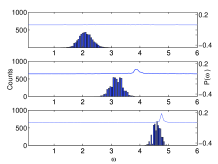
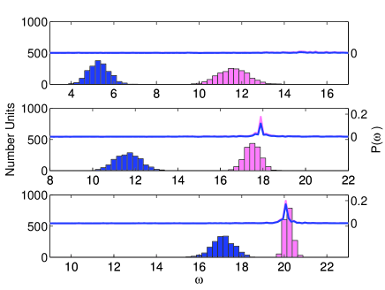
In particular, the threshold $a_{c}$ is marked by the onset of coherent temporal oscillations in the components of $\bm{P}(t)$. We characterize the microscopic underpinnings of these oscillations by considering $\bar{\omega_{i}}$, the time-averaged frequency of oscillator $i$ in the steady state. We perform simulations on globally coupled lattices of $N=3500$ units of a single population with $\gamma=1$ and also of a dichotomously disordered population with $\gamma_{1}=2.5$ and $\gamma_{2}=5.5$. As shown in Figs. 6 and 7, the distribution of frequencies $\bar{\omega_{i}}$ clusters around the values prescribed by $\gamma$ (or $\gamma_{1}$ and $\gamma_{2}$ for populations one and two, respectively) far below threshold (top panels). Specifically, for a deterministic oscillator with transition rate $\gamma$, $\bar{\omega_{i}}$ is given by $2\pi\gamma/3$; when $\gamma=1$ (or $\gamma_{1}=2.5$ and $\gamma_{2}=5.5$), this gives the central peak of the histogram for the relevant population. We compare these histograms with the power spectra $\left(\tilde{P}_{1,\gamma_{i}}(\omega)\tilde{P}^{*}_{1,\gamma_{i}}(\omega)\right)^{1/2}$, where $\tilde{P}_{1,\gamma_{i}}(\omega)$ is the Fourier transform of $P_{1,\gamma_{i}}(t)$. As threshold is eclipsed (middle panels), a peak arises in the power spectrum of the macroscopic variables $P_{1,\gamma_{i}}$, though the frequency of this peak does not correspond with the individual $\bar{\omega_{i}}$’s of oscillators constituting the population. In the dichotomous case, this peak only roughly corresponds with the time averaged frequencies from population two and completely exceeds even the maximum $\bar{\omega_{i}}$ characterizing population one. As $a$ is further increased, the descrepency between the time-averaged frequency histograms and the macroscopic oscillation frequencies decreases. In addition, in the disordered case, the histograms for the two populations become increasingly narrow and closer to one another (bottom panel). We note that as $a$ becomes tremendously large, the histograms become extremely narrow and begin to overlap at a frequency determined by the frequency of the macroscopic oscillations, as expected (indicative of perfect synchronization). Nonetheless, the behavior for finite, intermediate $a$ is rather counterintuitive and points to a rich microscopic dynamics underlying the cooperative behavior.

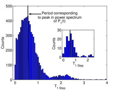
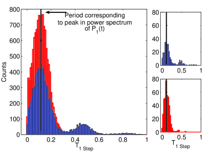
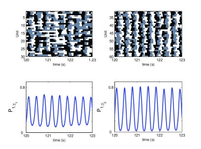
To further explore these trends, we consider the stochastic variable $T_{1~{}step}$, the waiting time in a single state for an individual oscillator. $T_{1~{}step}$ represents the time the oscillator spends in a single state $i$ before transitioning to the subsequent state $i+1$. For computational efficiency, we record $T_{1~{}step}$ for a representative subpopulation of $60$ units ($30$ units from each population, one and two, in the disordered case). Figures 8 and 9 show histograms of the variable $T_{1~{}step}$ taken over this representative subpopulation once steady state was reached. Clearly, all relevant subpopulations consist of oscillators whose steps most often correspond to the frequency of the macroscopic oscillation (shown by the solid vertical line). That is, the peak of the histograms occur at a value $T$ comensurate with the frequency peak in the power spectrum of the components of $\bm{P}(t)$. However, Fig. 8 shows that the distribution of $T_{1~{}step}$ is bimodal, with a significant peak occuring at $T_{1~{}step}\approx 2.2$ which downward biases the time-averaged frequencies $\omega_{i}$ of individual units. We note that as coupling $a$ increases significantly above threshold, the distribution becomes unimodal with a peak at $T_{1~{}step}$ corresponding to the frequency of macroscopic oscillation. In the disordered case, only population one, characterized by significantly lower time-averaged $\bar{\omega}$’s, shows a bimodal distribution with a significant peak at $T_{1~{}step}\approx 0.45$. In fact, these long waiting times, while not the dominant macroscopic behavior, pervade the microscopic dynamics in such a way that the time-averaged frequencies become downward biased and no longer accurately represent the macroscopic dynamics. Interestingly, population two has become sufficiently synchronized that the second peak is effectively nonexistent, and thus the frequencies overlap more closely with the macroscopic “mean field” frequency. The right insets of Figs. 8 and 9 show histograms for single units chosen from the populations (or subpopulations). Again, the unit chosen from the single population case shows a bimodal distribution with significant “anamolous” peaks near $T_{1~{}step}\approx 2.2$. In the disordered case, the unit from population one shows a bimodal waiting time distribution characterized by occasional waiting times in the neighborhood of $T\approx 0.45$ in addition to those corresponding to the macroscopic oscillations. Finally, in Fig. 10 we show the time evolution of the subpopulations along with the macroscopic variable $P_{1,\gamma_{i}}$ for each population. At any given time, the majority of oscillators in each population is synchronized, leading to the smooth oscillations of the macroscopic variable. However, isolated single units are prone to long waiting times, particularly in the less synchronized population (population one, left panel, in this example). These anamolously long waiting times, which serve to bias the time averaged frequencies $\bar{\omega_{i}}$ of each individual unit, nevertheless do not substantially disrupt the macroscopic oscillations, largely because the occurance of coincident long waits is fairly uncommon. That is, the long waiting times do not appear in any significantly correlated way among individual constituents of the population.

Figure 10: (Color online) The top panels show the evolution of a representative sub-system ($N=30$ units of each population). Dark, medium, and light represent states 1,2, and 3, respectively. The bottom panels show the macroscopic variable $P_{1,\gamma_{i}}$ for each population. The left panels correspond to population one ($\gamma_{1}=2.5$), while the right panels correspond to population two ($\gamma_{2}=5.5$). $a=3.60$ (above threshold) for all plots.

V Discussion

We have shown that a class of simple, discrete models of stochastic phase coupled oscillators can undergo either a subcritical or supercritical bifurcation to macroscopic synchrony, depending on the chosen form of the microscopic coupling. As such, the different instances of the model can be used to study either continuous phase transitions threestate1 ; threestate2 or discontinuous transitions exhibiting hysteresis, a characterstic seen in detailed theoretical models of, e.g., coupled Josephson junctions filatrella07 but only observed in significantly more complex coupled oscillator models daido ; gianuzzi07 ; filatrella07 ; tanaka ; acebron ; choi ; pazo ; hong0 . We stress that universality suggests that all models in this class exhibiting continous phase transitions should show similar behavior near the critical point, and this served as the basis of our eariler studies threestate1 ; threestate2 . Nevertheless, it is remarkable that minor modifications in microscopic coupling can alter the nature of the bifurcation in such a fundamental way.

In addition, we have shown that in dichotomously disordered populations, both subcritical and supercritical Hopf bifurcations can occur, and the distinction is completely determined by the relative width $\mu$ characterizing the transition rate disorder between the two populations. While the qualitative features of the transitions within each class (subcritical and supercritical) appear identical, the distinction between classes points to fundamentally different mechanisms underlying the initial emergence of phase synchronization. In particular, it is striking that the level of disorder within a population, as measured by $\mu$, can significantly alter the behavior near the critical point (though we stress that behavior even moderately above threshold is qualitatively indistinguishable).

Finally, we have studied the microscopic basis of phase synchronization above threshold. It is initially counterintuitive that phase synchronization, defined in terms of the Hopf bifurcation and temporal oscillations in the macroscopic variable $\bm{P}(t)$ (and measured in the order parameter $r$), is not contingent upon the existence of overlapping distributions of $\bar{\omega_{i}}$. That is, our results regarding the discrete oscillator model highlight the complexity of microscopic dynamics underlying macroscopic cooperation and point to a potentially misleading subtlety. Whereas phase synchronization is often considered a stronger condition than frequency entrainment – defined using an order parameter built upon the notion that a fraction of units display identical time-averaged frequencies in the oscillator population – we here report subtle microscopic features which distinguish the two without establishing a clear hierarchy. For example, Hong et al. hong show that for disordered populations of Kuramoto oscillators, the lower critical dimension for frequency entrainment is lower than that for phase synchronization in locally coupled oscillators, indicating the relative ease with which frequency entrainment is achieved. They note that the two transitions coincide in the case of globally coupled units. Contrast that with our dichotomously disordered population, for which phase synchronization occurs without any overlap in the frequency distributions: that is, no oscillator from population one has the same frequency as any oscillator from population two. While a direct comparison is not plausible owing to the specific differences between models and order parameters, we stress that any order parameter related to time-averaged measurements of frequencies would, for our model, be misleading and provide potentially counterintuitive results. The emergence of a nonzero $r$, which measures phase synchronization, corresponds with the loss of stability of the asynchronous fixed point (the Hopf bifurcation). This does not guarantee similar distributions of time-averaged frequencies in the two populations; in fact, we can readily see that synchronization occurs while the frequency distributions are entirely distinct. Furthermore, the frequency of the macroscopic oscillations of the mean field does not always coincide with the time-averaged frequencies of the oscillators constituting the population (or any subpopulation). Only when coupling is sufficiently large to substantially reduce the anamolously long waiting times which bias $\bar{\omega_{i}}$ will the frequency distributions begin to overlap one another and coincide with the frequency of the mean field oscillations. Because these long waiting times appear more readily in the population with the smaller $\gamma_{i}$, the time-averaged frequencies of the two populations are disproportionately affected, meaning that the populations will appear to behave quite differently in terms of average frequency. This in fact underlies the stark differences in the degree of synchronization between two populations as measured by the order parameter $r$, and provides an intuitive description capable of explaining this discrepancy. Our previous results show that completely disordered populations show qualitative similarities with the dichotomously disordered case threestate3 ; hence, we are led to cautiously speculate that wholly disordered populations are also characterized by waiting times $T_{1~{}step}$ distributed with long tails, and hence time-averaged frequencies become downwardly biased, meaning that the order parameter for frequency entrainment, in the typical sense, will not accurately reflect the macroscopic cooperation. Further studies along these lines are currently in progress.

Finally, the results of this work raise the following question: how dependent is the above phenomenon on the choice of a discrete phase model? Would similarly counterintuitve results arise in continous phase oscillators? In fact, a recent study by Rosenblum and Pikovsky rosenblum07 suggests that a similar (though not identical) state of partial synchronization arises in continous oscillators coupled in a highly nonlinear fashion. Specifically, they find that in globally coupled oscillators, phases exist in which certain subpopulations are characterized by time-averaged frequencies which are not commensurate with the oscillations of the mean field, that is, they are not locked with the macroscopic oscillations induced in the population. While once again the differences between the models make direct comparison difficult, it is nevertheless clear that measurements of time-averaged frequencies provide potentially counterintuitive results, even in globally coupled arrays. In the case of our stochastic discrete oscillators, the behvavior is quite transparent once viewed in terms of $T_{1~{}step}$, though it is not clear whether a similar mechanism underlies the phenomenon in the continous phase model. Uncovering the relationship between the superthreshold phase in our model and that in the continous oscillator model of rosenblum07 remains an open question, but even the superficial similarities between the results motivate continued efforts along these lines.

References

- (1) S. H. Strogatz, Nonlinear Dynamics and Chaos (Westview Press, 1994).
- (2) A. T. Winfree, J. Theor. Biol. 16, 15 (1967).
- (3) Y. Kuramoto, Chemical Oscillations, Waves, and Turbulence (Springer, Berlin, 1984).
- (4) S. H. Strogatz, Physica D 143, 1 (2000).
- (5) K. Wood, C. Van den Broeck, R. Kawai, and K. Lindenberg, Phys. Rev. Lett. 96, 145701 (2006).
- (6) K. Wood, C. Van den Broeck, R. Kawai, and K. Lindenberg, Phys. Rev. E 74, 031113 (2006).
- (7) K. Wood, C. Van den Broeck, R. Kawai, and K. Lindenberg, Phys. Rev. E, 041107 (2007).
- (8) F. Giannuzzi, D. Marinazzo, G. Nardulli, M. Pellicoro, and S. Stramaglia. Phys. Rev. E 75, 051104 (2007).
- (9) G. Filatrella, N. F. Pedersen, and K. Wiesenfeld. Phys. Rev. E 75, 017201 (2007).
- (10) H-A. Tanaka, A. J. Lichtenberg, and S. Oishi, Phys. Rev. Lett. 78, 2104 (1997).
- (11) J. A. Acebrón, L. L. Bonilla, and R. Spigler, Phys. Rev. E 62, 3437 (2000).
- (12) M. Y. Choi, H. J. Kim, D. Kim, and H. Hong, Phys. Rev. E 61, 371 (2000).
- (13) D. Pazó, Phys. Rev. E 72, 046211 (2005).
- (14) H. Hong, M. Y. Choi, B-G. Yoon, K. Park, and K-S Soh, J. Phys. A: Math. Gen. 32, L9 (1999).
- (15) H. Daido. Physica D 91, 24-66 (1996); Phys. Rev. Lett 73, 760 (1994).
- (16) Yu. A. Kuznetsov, Elements of Applied Bifurcation Theory, 2nd ed. (Springer, New York, 1998).
- (17) H. Hong, H. Park, and M. Choi, Phys. Rev. E 71, 054204 (2004); H. Hong, H. Park, and M. Choi, Phys. Rev. E 72, 036217 (2005).
- (18) M. Rosenblum and A. Pikovski. Phys. Rev. Lett 98, 064101 (2007).