Disease spreading in populations of moving agents

Abstract

We study the effect of motion on disease spreading in a system of random walkers which additionally perform long-distance jumps. A small percentage of jumps in the agent motion is sufficient to destroy the local correlations and to produce a large drop in the epidemic threshold, well explained in terms of a mean-field approximation. This effect is similar to the crossover found in static small-world networks, and can be furthermore linked to the structural properties of the dynamical network of agent interactions.

Many information/communication and social systems can be modeled as complex networks barabasireview ; newmanreview ; boccalettireview . One of the main reasons for studying such networks is to understand the mechanisms by which information, rumors and diseases spread over them. Recent works have pointed out the importance of incorporating the peculiar topology of the underlying network in the theoretical description of disease spreading anderson92 ; murray ; hethcote . Epidemic models are in fact heavily affected by the connectivity patterns characterizing the population in which the infective agent spreads. Both the nature of the final state, and the dynamics of the disease process, strongly depend on the coupling topology. Specifically, spreading occurs faster in small-world systems, i.e. in networks with shorter characteristic path lenghts wattsbook ; kuperman . Moreover, the epidemic threshold is affected by the properties of the degree distribution $P(k)$. For instance, the divergence of the second-order moment of $P(k)$ leads, in uncorrelated scale-free networks, to the surprising result of the absence of an epidemic threshold and its associated critical behavior pv00 ; moreno02 ; newman02 . This implies that scale-free networks are prone to the spreading of infections at whatever spreading rate the epidemic agents possess.

Most of the results present in the literature so far refer to cases where the disease spreading takes place over a wiring topology that is static, i.e. the underlying network is fixed in time, or grown, once forever. A more realistic possibility is to consider the networks themselves as dynamical entities. This means that the topology is allowed to evolve and adapt in time, driven by some external factors or by the very same spreading process. For instance, Refs.gross ; bagnoli have considered disease spreading on adaptive networks in which the susceptible agents have perception of the risk of infection, and are able to avoid contact with infected agents by rewiring their network connections. In this Letter we study disease spreading on a system of mobile agents. The agents are random walkers which can additionally perform long-distance jumps, and are only able to interact with agents falling within a given interaction radius apart from them. Hence, the interaction network between individuals is a dynamical one, because the links evolve in time according to the agent movement. The focus of our work is on the influence of the motion on the disease spreading. With the aim of large scale simulations, we will show that the motion, usually neglected in epidemic models, has instead a profound effect on the dynamics of the spreading and on the epidemic threshold. In particular, a small number of long-distance jumps in the agent motion is sufficient to produce a large drop in the epidemic threshold, as that observed in static small-world networks kuperman . The case of infecting moving individuals has been considered only in few other works Boccara92 ; gonzalez04 ; eubank04 ; colizza06 ; frasca06 ; nekovee07 , although the effects on the epidemic threshold have never been studied in detail before. This is a quite important issue both in social and in artificial networks. E.g., recently the analogy with epidemic spreading has been exploited to propose routing algorithms in highly mobile networks of computers Neglia05 ; mascolo06

We consider a system of $N$ identical agents independently moving in a two-dimensional cell of linear size $D$, with periodic boundary conditions. Fixing the value of $D$ is equivalent to fix the agent density $\rho=N/D^{2}$. The agents are represented as point particles, and their positions and velocities at time $t$ are indicated as $\mathbf{r}_{i}(t)$ and $\mathbf{v}_{i}(t)\equiv(v_{i}(t)\cos\theta_{i}(t),v_{i}(t)\sin\theta_{i}(t))$, $i=1,...,N$. We further impose that the agents move with a velocity modulus which is constant in time and equal for all the agents, i.e. $v_{i}(t)=v,\forall i=1,..,N$ and $\forall t$. At time $t=0$ the $N$ particles were distributed at random. At each time step, the agents change stochastically the direction angles $\theta_{i}(t)$. The positions and the orientations of the particles are thus updated according to the following rule:

$$\theta_{i}(t) = \xi_{i}$$

$$\mathbf{r}_{i}(t+1) = \mathbf{r}_{i}(t)+\mathbf{v}_{i}(t)$$ (1)

where $\xi_{i}$ are $N$ independent identically distributed random variables chosen at each time with uniform probability in the interval $[-\pi,\pi]$. In addition, to include the possibility that agents can move through the bidimensional world with time scales much shorter than those related to disease, as in the case of infected individuals travelling by flights colizza06 , we consider that agents can perform long-distance jumps. This is accounted for by defining a parameter, $p_{j}\in[0,1]$, that quantifies the probability for an agent to perform a jump into a completely random position. In summary, at each time step, each agent evolves: following Eqs. (1), with a probability $1-p_{j}$, or performing a jump, with probability $p_{j}$. In the latter case the position of the agent is updated into a new position chosen at random in the cell. Models with different jumping rules frasca06 , non-indentical and interacting agents, have also been considered, and the results will be reported elsewhere. Finally, the main parameters controlling the moving agents in our model are: $\rho$, $v$ and $p_{j}$.

Among the possible mechanisms of disease spreadings anderson92 ; murray ; hethcote , we focus on the SIR model, that divides the $N$ agents into three disjoint groups: susceptible (S), infective (I) and recovered (R). We indicate as $N_{S}(t)$, $N_{I}(t)$ and $N_{R}(t)$, respectively, the number of agents in the three groups at time $t$, with the total number of agents $N_{S}(t)+N_{I}(t)+N_{R}(t)=N$ being constant in time. A small number of agents is set in the infective state at $t=0$ as the seed of the infection, while all the others start from the susceptible state. The process through which the disease spreads can be summarized as following. An interaction radius $r$ is fixed ($r=1$ in all our calculations), and this defines the interaction network: at each time step $t$ each agent interacts only with those agents located within a neighborhood of radius $r$. For a given susceptible agent, the probability of being infected increases with the number of infected individuals in the neighborhood. More precisely, if an agent is in the $S$ state at time $t$, and exactly one of its neighbors is in the $I$ state, then it moves into the $I$ state with probability $\lambda$ and stays in the $S$ state with probability $1-\lambda$. If $N_{I_{r}}$ is the number of infected individuals in the neighborhood of the agent, then its probability of being infected is $1-(1-\lambda)^{N_{I_{r}}}$. In addition to this, each infected agent can move into the $R$ state with probability $\mu$, and then cannot catch the disease anymore. This sets the average duration time of the infection: $\tau=\frac{1}{\mu}$.

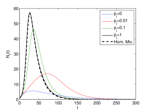
In our model we implement the motion rules and we update, at each time step, the disease state of every agent. The model is simulated for a number of time steps sufficiently high to ensure that, at the end, there are no more infected individuals in the population. During a simulation, the number $N_{I}(t)$ of infected grows up, reaches a peak value, and then decreases. Typical cases are shown in Fig. 1,

Figure 1: (Color online). Number of infected individuals as a function of time $t$. We have considered a system with $N=1000$, $\rho=1$, $v=0.1$, $\lambda=0.1$, $\mu=0.05$ and different values of $p_{j}$. The system is started with $1\%$ of the agents set in the infective states. Results are averages over 100 runs. The dashed line is the result in the homogeneous mixing approximation of Eqs. (2)

where it can be noticed that a larger value of $p_{j}$ increases the spread of the infection. In fact, the peak of infected individuals is higher in the presence of a larger probability of jumping. We have verified that this is also true for the total number of individuals which have contracted the disease at the end of the process. Both the two issues have important practical consequences, since on one hand the disease involves a higher percentage of the population, and, on the other hand, it requires more resources to deal with a higher peak of infected individuals.

The behavior for large $p_{j}$ and/or large $v$ can be interpreted in terms of a mean-field approximation. In fact, in such limit, we expect that the spatial correlations in the disease states are destroyed by the agent motion, and we assume that the homogeneous mixing (HM) hypothesis is valid. Under this hypothesis, all the individuals have the same probability of contacting any other individual (i.e., the population mixes at random) anderson92 ; murray ; hethcote ; Boccara92 , and the equations for the system of infectious mobile agents read:

$$i(t+1) = i(t)+s(t)\left[1-\left(1-\lambda i(t)\right)^{a}\right]-\mu i(t)$$

$$r(t+1) = r(t)+\lambda i(t)$$ (2)

$$s(t+1) = \rho-i(t+1)-r(t+1)$$

where $s(t)=N_{S}(t)/D^{2}$, $i(t)=N_{I}(t)/D^{2}$, $r(t)=N_{R}(t)/D^{2}$, are respectively the densities of susceptible, infected and recovered individuals at time $t$, and $a=\pi r^{2}$. The third equation is simply derived from the conservation of the number of agents. The second equation indicates that the increase of recovered individuals at time $t+1$ is proportional to the number of infected individuals which get recovered, i.e. to $\lambda i(t)$. The first equation can be derived by taking into account that the density of infected individuals at time $t+1$ is decreased by $\lambda i(t)$ and increased by the density of susceptibles catching the disease. This last term is proportional to $s(t)$ times a contagion probability $p_{cont}$. The contagion probability is given by $p_{cont}=1-\bar{p}_{cont}$, where $\bar{p}_{cont}$ represents the probability of not being infected. $\bar{p}_{cont}$ is the probability that an agent will not being infected by none of its neighbors, i.e. $\bar{p}_{cont}=\left(1-\lambda\frac{N_{I}(t)}{D^{2}}\right)^{a}$, with $a$ representing the area in which each agent may sense other infective individuals, that in our case is equal to $\pi r^{2}$. The number of infective agents as a function of the time in the HM approximation computed from Eqs. (2), with $\lambda=0.1$ and $\mu=0.05$, is reported as a dashed line in Fig. 1. As expected, the curves for the model approach the dashed line when $p_{j}\rightarrow 1$. The mean field approach gives us also information on the epidemic threshold. In fact, for small $i(t)$ we can approximate $\left(1-\lambda i(t)\right)^{a}\simeq 1-a\lambda i(t)$, and we get from Eqs. (2) the iterative rule $i(t+1)=i(t)+\pi r^{2}\lambda s(t)i(t)-\mu i(t)$. This allows to distinguish two cases. In fact, by assuming $s(0)\simeq\rho$, we get $i(1)>i(0)$ when $\sigma\equiv\lambda/\mu>\frac{1}{\pi r^{2}\rho}$, while $i(1)<i(0)$ when $\sigma\equiv\lambda/\mu<\frac{1}{\pi r^{2}\rho}$. Thus, under the HM hypothesis we derive a critical threshold:

$$\sigma_{c}=\frac{1}{\pi r^{2}\rho}$$ (3)

Hence, when $\sigma<\sigma_{c}$, the number of infected decrease monotonically, while for $\sigma>\sigma_{c}$ an epidemic outbreak occurs. Also notice that $\sigma_{c}=\frac{1}{<k>}$ as found in Erdős and Rényi random graphs newmanreview ; boccalettireview , where $<k>$ is the average number of first neighbours of an agent, that in our case is equal to $\rho\pi r^{2}$.

Figure 2: (Color online). Epidemic threshold as a function of the system density $\rho$. We have considered $N=1000$, $v=0.1$, and $\mu=0.05$. Different curves correspond to different values of $p_{j}$. Results are averages over 100 runs. The dashed line is the prediction in the homogeneous mixing approximation.

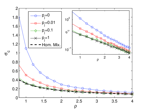
In Fig. 2 we report the epidemic thresholds $\sigma_{c}$ computed numerically for the model of infective agents moving with different values of $p_{j}$. For a given density $\rho$, We observe that $\sigma_{c}$ is a decreasing function of the density $\rho$. Moreover, for a given value of $\rho$, the threshold decreases with the jumping probability $p_{j}$. In the same figure we report for comparison the prediction of Eq. (3), as a dashed line. We notice that the homogeneous mixing approximation becomes more and more accurate when $p_{j}$ tends to 1. The convergence to the HM threshold of Eq. (3) as a function of $p_{j}$ is rather fast. For instance, already at $p_{j}=0.1$, the threshold in the model is, for any value of $\rho$ reported, practically indistinguishable from the HM one. In Fig. 2 we have considered a fixed velocity $v=0.1$. We have also studied $\sigma_{c}$ as a function of $v$, at a fixed density and for different values of $p_{j}$. We observed that for small values of $v$, the epidemic threshold tends to the prediction of the HM when $p_{j}$ tends to 1, while, for large enough values of $v$, the epidemic threshold is consistent with the homogenous mixing one, independently of $p_{j}$.

Figure 3: (Color online). Scaled epidemic threshold $\sigma_{c}(p_{j})/\sigma_{c}(p_{j}=0)$ as a function of $p_{j}$. We have considered $v=0.1$ and $\mu=0.05$. Different curves correspond to different values of the density $\rho$. Results are averages over 100 runs.

Finally we investigate in more details the effects of $p_{j}$ on the epidemic threshold. In Fig. 3 we report, as a function of $p_{j}$, the value of the threshold $\sigma_{c}(p_{j})$, normalized by $\sigma_{c}(p_{j}=0)$, for different values of the density $\rho$. We observe a rapid drop in the curves (note the logarithmic scale for $p_{j}$), meaning that a small number of long-range jumps produce a large decrease in the epidemic threshold. The plateau observed for $p_{j}$ larger than $10^{-2}$ implies that in order to have a significant change in the epidemic threshold (and in the disease incidence) in our model of moving agents, the jumping probability has to be extremely small. This is in line with other results, stressing the role of the large scale properties of the airline transportation networks in determining the global diffusion pattern of emerging diseases colizza06 , and can have important implications in the immunization of real communication networks gomez06 . Different curves in the figure correspond to different densities. As $\rho$ decreases, the drop in the curve occurs for smaller and smaller values of $p_{j}$, suggesting that no finite critical value of $p_{j}$ can be determined this way. This behavior is similar to the crossover observed in the characteristic path length of small-world networks as a function of the rewiring probability wattsbook ; Barrat00 . We notice, however, that in our case the effect is due to the agent movement and not to the rewiring of static links.

Figure 4: Characteristic path length $L_{G}$ (circles) and clustering coefficient $C_{G}$ (squares) as a function of $p_{j}$ ($N=1000$, $\rho=1$, $v=0.1$). Results are averages over 10 realizations.

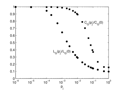
The observed behaviour can be related to the topological properties of the underlying dynamical network. For such purpose we define an effective adjacency matrix $G_{\tau}(t)=\{g_{ij}(t)\}$ taking into account that each infected individual may infect other individuals during the average duration of the infection, i.e. during $\tau=\frac{1}{\mu}$ simulation steps frasca06 . Let $A(t)$ be the adjacency matrix at time $t$ defined so that $a_{ij}(t)=1$ if the $j^{th}$ agent is within the interaction radius of the $i^{th}$ agent at time $t$, and $a_{ij}(t)=0$ otherwise. We set $g_{ij}(t)=1$, if at least for one $t^{\prime}$, with $t^{\prime}=t,t-1,\cdots,t-\tau+1$, it is verified that $a_{ij}(t^{\prime})=1$. Otherwise we set $g_{ij}(t)=0$. In Fig. 4 we report the characteristic path length, $L_{G}$, and the clustering coefficient, $C_{G}$ of matrix $G(t)$ as a function of $p_{j}$. The behavior we observe is in all similar to that found in small-world networks for increasing rewiring probability wattsbook . Notice that the drop in $L_{G}$ occurs at the same value of $p_{j}$ at which we have found the drop in the epidemic threshold.

In summary, we have considered a system of infectious mobile agents to study the effects of long-range moves on the disease spreading. Our results indicate that the interplay between dynamics and topology can have important consequences for the global spreading of infectious diseases in systems of mobile agents, and in the related applications such as the forecast of epidemic spreading and the development of wireless routing strategies.

References

- (1) R. Albert and A.-L. Barabási, Rev. Mod. Phys. 74, 47 (2002).
- (2) M.E.J. Newman, SIAM Review 45, 167 (2003).
- (3) S. Boccaletti, V. Latora, Y. Moreno, M. Chavez and D -U Hwang, Phys. Rep. 424 175 (2006).
- (4) R. M. Anderson and R. M. May, Infectious diseases in humans (Oxford University Press, Oxford, 1992).
- (5) J. D. Murray, Mathematical Biology (Springer Verlag, Berlin, 1993).
- (6) H.W. Hethcote, SIAM Review 42, 599 (2000).
- (7) D.J. Watts, Small Worlds: The Dynamics of Networks between Order and Randomness,(Princeton University Press, Princeton, New Jersey, 1999).
- (8) M. Kuperman and G. Abramson, Phys. Rev. Lett. 86, 2909 (2001).
- (9) R. Pastor-Satorras and A. Vespignani. Phys. Rev. Lett. 86, 3200 (2001).
- (10) Y. Moreno, R. Pastor-Satorras, and A. Vespignani, Eur. Phys. J. B26, 521 (2002).
- (11) M. E. J. Newman, Phys. Rev. E66, 016128 (2002).
- (12) T. Gross, C. J. D. D’Lima and B. Blasius, Phys. Rev. Lett. 96, 208701 (2006)
- (13) F. Bagnoli, P. Lió and L. Sguanci, arXiv:0705.1974; L. Sguanci, P. Lió and F. Bagnoli, arXiv:q-bio/0607010.
- (14) N. Boccara and K. Cheong, J. Phys. A25, 2447 (1992)
- (15) M.C. Gonzalez and H. J. Herrmann, Physica A340 741 (2004)
- (16) S. Eubank, H. Guclu, V. S. A. Kumar, M. V. Marathe, A. Srinivasan, Z. Toroczkai and N. Wang, Nature 429, 180 (2004)
- (17) V. Colizza, A. Barrat, M. Barthelemy and A. Vespignani, Proc. Natl. Acad. Sci. 103, 2015 (2006).
- (18) M. Frasca, A. Buscarino, A. Rizzo, L. Fortuna and S. Boccaletti, Phys. Rev. E74, 036110 (2001).
- (19) M. Nekovee, New Journal of Physics 9, 189 (2007).
- (20) E. Zhang, G. Neglia, J. Kurose and D. Towsle, Computer Networks 51, 2867 (2007).
- (21) M. Musolesi and C. Mascolo, in Proceedings of Int. Conference on Mobile and Ubiquitous Systems: Networks and Services (MOBIQUITOUS 2006). San Jose, CA. July 2006. ACM.
- (22) J. Gomez-Gardenes, P. Echenique and Y. Moreno, Eur. Phys. J. B49, 259 (2006).
- (23) A. Barrat, M. Weigt, Eur. Phys. J. B13, 547 (2000).