Matched-filtering and parameter estimation of ringdown waveforms
Abstract
Using recent results from numerical relativity simulations of non-spinning binary black hole mergers we revisit the problem of detecting ringdown waveforms and of estimating the source parameters, considering both LISA and Earth-based interferometers. We find that Advanced LIGO and EGO could detect intermediate-mass black holes of mass up to out to a luminosity distance of a few Gpc. For typical multipolar energy distributions, we show that the single-mode ringdown templates presently used for ringdown searches in the LIGO data stream can produce a significant event loss ( for all detectors in a large interval of black hole masses) and very large parameter estimation errors on the black hole’s mass and spin. We estimate that more than templates would be needed for a single-stage multi-mode search. Therefore, we recommend a “two stage” search to save on computational costs: single-mode templates can be used for detection, but multi-mode templates or Prony methods should be used to estimate parameters once a detection has been made. We update estimates of the critical signal-to-noise ratio required to test the hypothesis that two or more modes are present in the signal and to resolve their frequencies, showing that second-generation Earth-based detectors and LISA have the potential to perform no-hair tests.
pacs:
04.70.-s, 04.30.Db, 04.80.Cc, 04.80.NnI Introduction
Astronomical observations provide us with a large number of black hole candidates Narayan:2005ie . Stellar mass candidates (with mass ) are found in X-ray binaries in our galaxy. Since the discovery of quasars and other active galactic nuclei, we have growing evidence that supermassive black holes (SMBHs, with ) should reside in the cores of almost all galaxies, including our own. There is also mounting observational support to the idea that intermediate-mass black holes (IMBHs) may fill the gap between these two classes of astrophysical objects.
It is commonly believed that the ultimate test of the “black hole hypothesis” will come from gravitational wave observations (see eg. Lasota’s entertaining account of exotic alternatives to astrophysical black holes Lasota:2006jh , and Hughes’ lectures Hughes:2005wj for a relativist’s perspective on present and future observational tests of the black hole hypothesis). From the point of view of an astrophysicist, black holes are not particularly interesting: “black hole candidates” are characterized only by their mass and angular momentum, and no compact object with mass has shown any feature that would allow us to attribute to it any other property other than mass and rotation. For a relativist, black holes (being vacuum solutions of the field equations) are much more exciting: they are unique, “clean” probes of the structure of spacetime in strong-gravity conditions.
An important identifying dynamical feature of a black hole are its characteristic damped oscillation modes, called quasinormal modes (QNMs) kokkotasnollert . Any compact binary merger leaving behind a black hole produces a gravitational wave signal that, after the black hole’s formation, can be decomposed as a superposition of exponentially damped sinusoids. By analogy with the ordinary vibrations of a bell, this signal is known as “quasinormal ringing” or ringdown.
The fact that all information is radiated away in the process leading to black hole formation, so that astrophysical black holes in Einstein’s theory are characterized completely by their mass and angular momentum, is known as the “no-hair theorem”. For this reason the ringdown signal is very simple: mass and angular momentum are enough to characterize the black hole’s oscillation spectrum (see Ref. bcw for details), and the detection of ringdown waves may allow us to identify a black hole and determine its properties. A measurement of the frequency and damping time of a single QNM can be used, at least in principle (see below), to determine both the mass and angular momentum of the hole echeverria ; finn ; Flanagan:1997sx ; bcw . Detection of more than one QNM would allow us to test consistency with the black hole hypothesis – or in more colloquial speaking, to “test the no-hair theorem” Dreyer:2003bv ; bcw .
The detectability of ringdown waves, as well as their use to measure black hole properties and test relativity, depend mainly on two factors: (i) the fraction of the black hole’s mass radiated in ringdown waves (i.e. the “ringdown efficiency” ), and (ii) the detector’s sensitivity in the frequency band of interest. In Ref. bcw , some of us carried out a detailed study of ringdown detectability and no-hair tests with the planned space-based Laser Interferometer Space Antenna (LISA). The ringdown efficiency , the multipolar energy distribution of the radiation and the dimensionless angular momentum of the final black hole were considered as free parameters, to be varied within a certain reasonable range. We confirmed and refined earlier estimates by Flanagan and Hughes Flanagan:1997sx , showing that the ringdown signal-to-noise ratio (SNR) is usually larger than the inspiral SNR for the typical SMBH masses () inferred from astronomical observations of nearby galaxies.
Binary black hole simulations are now carried out by different groups all over the world. Large-scale simulations of non-spinning unequal-mass binary black hole mergers were recently used to provide reliable estimates of , of the final angular momentum and of the multipolar energy distribution Berti:2007fi . Ref. Berti:2007fi also showed that two or more modes are excited to comparable amplitudes in a binary black hole merger whenever the binary’s mass ratio . The significant excitation of different multipolar components can be used to extract useful information on the geometry of the ringing object, and to perform no-hair tests (in the sense explained above).
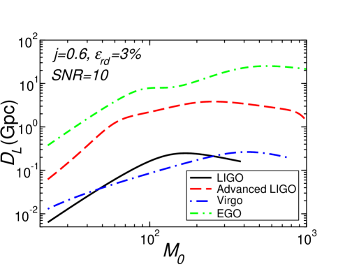
In this paper we revisit the analysis of Ref. bcw taking into account these recent results from numerical relativity, and we extend that study to include planned and presently operating Earth-based detectors (LIGO, Virgo, Advanced LIGO and EGO). Many authors have recently stressed the potential of Earth-based detectors for measuring ringdown waves in the IMBH mass range Cutler:2002me ; Fregeau:2006yz ; Buonanno:2006ui ; Pan:2007nw ; Baker:2006kr ; Ajith:2007qp ; Luna:2006gw ; Mandel:2007hi ; Belczynski:2004gu ; Kulczycki:2006ht ; Wyithe:2003ju . For example, Ref. Pan:2007nw matched an equal-mass merger waveform from numerical relativity to a Post-Newtonian inspiral and showed that the resulting SNR for a single LIGO detector peaks at , which is well within the IMBH mass range. The results presented in this paper confirm that ringdown waves may be used to provide conclusive evidence for the existence of IMBHs and (even more importantly) to accurately measure their parameters. Initial LIGO (Virgo) may detect IMBHs with (, respectively) out to a luminosity distance Mpc. Advanced Earth-based interferometers would extend the luminosity distance at which ringdown events are detectable by a factor for Advanced LIGO, and for EGO (see Fig. 2 below). Advanced LIGO and EGO could detect IMBH ringdowns out to cosmological distances with large SNR, and allow precision measurements of the IMBHs’ properties.
Higher multipolar components of the radiation can be significantly excited Berti:2007fi , and this calls for a critical revision of the matched-filtering techniques used for ringdown searches. Present ringdown searches in the LIGO data stream use templates consisting of only one QNM goggin (see also Ref. Clark:2007xw for data analysis methods to resolve neutron star ringdowns from instrumental glitches).
In this paper we address this problem and give a preliminary answer to the following questions:
-
(1)
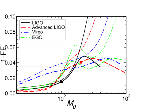
Given estimates of the multipolar energy distribution in non-spinning binary black hole mergers, how many events would we miss in a search with single-mode ringdown templates? The answer is quantified in Fig. 1, where we compute Owen’s “minimal match” Owen:1995tm as a function of the black hole mass measured in the source frame. The event loss is larger than whenever the minimal match is larger than (details are provided in the body of the paper). From the figure we see that this happens in a significant mass range for all Earth-based detectors. We will show below that similar conclusions apply also to the planned space-based interferometer LISA, although in a completely different mass range. Furthermore, we will show that single-mode templates can produce a large bias in the estimation of the black hole’s mass and spin. Our conclusions should be rather conservative, because from perturbation theory and from numerical relativity results we expect higher multipoles to be more excited for black hole binaries with spin and large mass ratios.
-
(2)
How many templates would we need for searches using two-mode templates? We estimate that, as compared with single-mode searches, the number of templates needed for a two-mode search would increase by roughly three orders of magnitude. A more detailed data analysis study (eg. using better template placing techniques, along the lines of nakano ) could be useful to reduce computational requirements.
-
(3)
How strong must a ringdown event be if we want to perform no-hair tests or resolve nonlinear contributions Ioka:2007ak to the ringdown waveform? More precisely: what is the minimum SNR needed to resolve QNMs? Below we address different aspects of this problem (frequency, damping time and amplitude resolvability require different SNRs). Our results suggest that prospects to resolve QNMs are quite optimistic for both LISA and second-generation Earth-based detectors.
The plan of the paper is as follows. In Sec. II we discuss the potential of Earth-based detectors to measure ringdown waves from solar-mass black holes and IMBHs. In Sec. III we look at the event loss and bias in parameter estimation induced by searching for a two-mode waveform with a single-mode template. In Sec. IV we revise our previous estimates bcw of the critical SNR required to perform no-hair tests. Sec. V contains a brief summary of our conclusions. Some technical details are presented in the Appendices. In Appendix A we estimate the number of templates required to detect multi-mode waveforms, and in Appendix B we provide a (somewhat optimistic) estimate of the critical SNR required to test the hypothesis that two modes are present in a ringdown signal.
II Ringdown detectability by Earth-based detectors
In this Section we study the detectability of ringdown waves by present and planned Earth-based interferometers: LIGO, Virgo, Advanced LIGO and EGO. Our analysis complements that of Ref. bcw , where a similar study was performed for the planned space-based interferometer LISA. Detectability can be assessed by computing the (maximum) SNR achievable by matched-filtering:
| (1) |
where the scalar product between two waveforms is defined as finn ; Apostolatos:1995pj
| (2) |
Here
| (3) |
is the Fourier transform of the waveform , and is the noise power spectral density (PSD) of the detector. For the initial LIGO and Virgo PSD we use the analytic approximation of Ref. Damour:2000zb . We assume that the PSD for , where the low-frequency sensitivity cutoff Hz (for initial LIGO) and Hz (for Virgo). For Advanced LIGO we consider the broadband configuration PSD given in Ref. AdLIGO , and for the projected PSD of EGO we follow Appendix C of Ref. ego . For LISA, we model the PSD (including white-dwarf confusion noise) by the semianalytic approximation used in Berti:2004bd ; bcw , with a low-frequency cutoff Hz.
An estimate of the maximum detectable black hole mass for LISA and Earth-based detectors can be obtained by equating the fundamental QNM frequency (as tabulated and fitted in Ref. bcw ) to . Since QNM frequencies scale as , this sets a limit on the maximum detectable black hole mass. The results of this estimate, which are mildly dependent on the black hole’s rotation parameter , are listed in Table 1. The mass range accessible to Earth-based interferometers can increase dramatically with relatively small (but technically difficult) improvements in the low-frequency sensitivity threshold. For example, a detector with =10 Hz can detect IMBHs with even if they are non-spinning. For the typical spins that should result from a binary black hole merger (), a low-frequency sensitivity threshold at Hz means that initial LIGO will not be sensitive to QNM ringing from IMBHs with mass . The detectable mass range increases as the spin of the remnant black hole gets larger.
| Earth-based | ||||
|---|---|---|---|---|
| LISA |
 |
 |
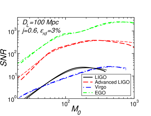
In the left panel of Fig. 2 we show the typical sky-averaged SNR of Earth-based detectors for black hole ringdowns at luminosity distance Mpc as a function of the black hole mass in the source frame (related to the mass in the detector frame by , where is the cosmological redshift). The actual value of the ringdown SNR changes slightly depending on the way we compute the Fourier transform in (3). There are two common conventions in the literature (see Ref. bcw for more details). The Echeverria-Finn (EF) convention (in the terminology of Ref. bcw ) is shown by thin lines in the left panel. It assumes that the ringdown waveform is zero before some starting time (say ). Alternatively, we can adopt the Flanagan-Hughes (FH) doubling prescription (thick lines in the figure): we assume that the waveform for is identical to that for except for the sign of (i.e., we replace by ) and we divide the resulting SNR by to compensate for the doubling Flanagan:1997sx . The left panel of Fig. 2 shows that adopting one or the other convention does not change the results significantly. In the remainder of the paper, we will adopt the EF convention, since it is generally more straightforward to implement in matched-filtering applications.
The right panel of Fig. 2 shows the luminosity distance out to which ringdown would be detectable by each detector with a SNR of 10 (assuming a flat, -dominated cosmology, in accordance with the latest observational data). In the Figure we use typical values from simulations of non-spinning binary black hole mergers Berti:2007fi , assuming that the final black hole has angular momentum and that the ringdown efficiency is . The results would not change much had we made different assumptions. In particular, the SNR scales with efficiency as . If the merging black hole binary has mass ratio , the ringdown SNR would decrease (to a very good approximation) by a factor compared to the equal-mass case Berti:2007fi . Fig. 2 can be compared with Figs. 7 and 8 in Ref. bcw , showing the inspiral and ringdown SNR of LISA at different values of the cosmological redshift (for clarity, in Fig. 2 we do not show the inspiral SNR). We also note that Figure 2 assumes matched filtering with one mode only, and that (following results from numerical relativity simulations) we assumed this mode to be the fundamental mode with . Inclusion of higher multipoles, the main topic of this paper, would only increase the sky-averaged SNR by small factors of order unity, but (as we will show) it may have important implications for a matched-filtering detection of the signal.
The left panel of Fig. 2 is in good agreement with the results for LIGO and Advanced LIGO shown in Fig. 2 of Ref. Fregeau:2006yz . Our results for Advanced LIGO are slightly different because we use a more accurate model for the PSD. For Virgo, our results agree with those in Ref. Kulczycki:2006ht . The right panel clarifies the potential of present and future interferometric detectors to detect ringdown waves. At the present sensitivity, LIGO could detect waves from IMBHs of mass out to a distance of about Mpc. Virgo spans roughly the same distance range, but it should be able to detect larger IMBH masses when the low-frequency design sensitivity is met. Advanced LIGO will extend the distance range out to a few Gpc (a factor ) and it should be able to detect IMBHs of mass . EGO would be a remarkable tool to detect IMBHs of mass as large as out to distances of Gpc and larger, and to measure their properties with remarkable precision.
III Event loss and bias in parameter estimation using single-mode templates
A common choice to search for signals of known form in noisy data is matched-filtering. Matched-filtering works by cross-correlating the signal with a set of theoretical templates222For alternative techniques especially designed to extract damped sinusoidal signals from noise, see Ref. bcgs and references therein.. Current searches for ringdown signals in the LIGO data stream goggin and in resonant bar detectors Pai make use of the simplest theoretical model: a single damped sinusoid. Here we try to assess the performance of such a template to detect a superposition of damped sinusoids. More precisely, we estimate the number of events we would miss by using single-mode templates to detect multi-mode signals, and we try to quantify the bias in measured parameters induced by the use of such templates.
The optimal way of addressing the performance of single-mode ringdown templates would be to use our present best guess for the “true” waveform emitted by a binary black hole merger: the wavetrain obtained by stitching together the Post-Newtonian predictions for the inspiral and the best available numerical relativity waveforms. Finding the optimal way to perform this stitching is in itself a difficult problem, now actively pursued by many research groups Buonanno:2006ui ; Pan:2007nw ; Baker:2006ha ; Berti:2007fi . Our purpose here is to make some general points of principle, exploring semi-quantitatively the typical event loss and parameter bias induced by single-mode templates. For this reason, and to keep the analysis as simple and general as possible, our “true” waveform will be taken to consist of a two-mode QNM superposition. Therefore we assume that the following two-mode signal is impinging on the detector, starting at time :
| (4a) | |||||
| (4b) | |||||
Here () denotes the oscillation frequency of each QNM, is the quality factor of the oscillation, and is the oscillation amplitude of mode . For reasons that will become apparent in the following, in the second line we found it convenient to express the signal in terms of the relative amplitude of the two modes . The Fourier transform of Eq. (4) in the EF convention reads:
| (5) |
Matched-filtering works by cross-correlating the detector’s output with a set of templates. Consider a one-mode bank of templates such as those presently used in ringdown searches goggin :
| (6) |
where is an (-dimensional) vector of template parameters, and for . In this particular case, and (in principle we could use as an additional parameter, but we verified by explicit calculations that setting doesn’t sensibly affect the fitting factor and the estimated values of the other parameters). The Fourier transform of this template is similar to those in Eq. (5), with an additional exponential factor depending on the starting time :
| (7) |
The performance of the template (6) to detect the two-mode waveform (4) can be computed with the help of the fitting factor (FF) first introduced by Apostolatos Apostolatos:1995pj :
| (8) |
where the scalar product between two waveforms has been defined in Eq. (2). An equivalent quantity often used in the literature is Owen’s “minimal match”, defined as Owen:1995tm . From the definition, Eq. (8), it is clear that an overall normalization constant (say, ) does not affect calculations of the FF: this is the reason for introducing the relative amplitude defined in (4). The FF measures the degradation of the SNR due to cross correlating an arbitrary signal , such as the two-mode signal (4), with all filters in the template bank. The effective SNR that can be obtained by matched-filtering is
| (9) |
where has been defined in Eq. (1). For gravitational wave detection the SNR is proportional to the inverse of the luminosity distance to the source, while the event rate (scaling with the accessible volume) is proportional to the cube of this distance. Therefore, given the FF, we can compute the event loss as
| (10) |
For detection purposes one usually requires , corresponding to a loss of less than of the events that could be potentially be detected by a “perfect” filter.
We compute the integrals in (8) and (9) using a Gauss-Legendre spectral integrator, and we perform the maximization by a Fortran implementation of the Nelder-Mead downhill simplex method numrec . In actual searches, the set of all templates forms a grid that should cover the -dimensional parameter space. The point on this grid for which the FF is maximum singles out the template that best matches the actual waveform impinging on the detector. If the FF is above some pre-determined threshold, eg. , we say that we have a detection. An estimate of the number of templates required to detect multi-mode waveforms is given in Appendix A.
The detectability of a multi-mode signal by a single-mode template depends, among other things, on the relative amplitude of the subdominant modes in the “real” signal. In our simplified signal (4) we denoted this relative amplitude by . Below we discuss how recent numerical simulations of binary black hole mergers can be used to provide such an estimate.
Estimates of the relative mode amplitude from numerical relativity
Recent results from numerical simulations of the merger of non-spinning, unequal mass black hole binaries support the expectation that the mode should dominate the ringdown signal Berti:2007fi . However, they also reveal that other modes (especially and ) are significantly excited. Whenever the mass ratio , the mode is excited to roughly one third of the amplitude of the mode. We expect this estimate of the relative excitation to be conservative: perturbative results and numerical simulations indicate that higher multipoles should be more excited as the the binary’s mass ratio grows, or when the black holes in the binary are spinning.
Merger simulations show that the projection of the Weyl scalar onto spin-weighted spherical harmonics has a circular polarization pattern (see Appendix D of Ref. Berti:2007fi ). In the ringdown regime the Weyl scalar can further be decomposed as a QNM sum, and to a good approximation we can write:
| (11) |
For simplicity, in this expansion we are considering only the least damped, fundamental mode for each pair bcw . We also approximate spin-weighted spheroidal harmonics by spin-weighted spherical harmonics, which introduces an error of order or less Berti:2005gp . The variable , with a constant, and it is implicitly assumed that all frequencies and damping times depend on the angular numbers . Using the equatorial symmetry of the system, the waveform can be rewritten as
| (12) |
where we have defined the following useful quantities:
| (13a) | |||||
| (13b) | |||||
Recalling that and using the large- limit, which is usually a good approximation bcw , we get
| (14a) | |||||
| (14b) | |||||
The gravitational wave strain at the detector is given by
| (15) |
where are pattern functions depending on the orientation of the detector and on the direction of the source, whose expressions can be found (for example) in Ref. thorne . In the following, to simplify the notation, we will drop the functional dependence of and on the angles.
Let us consider, for simplicity, a two-mode situation. Guided by numerical results for the merger phase (see below) we can assume that the dominant modes are and . Then we get
| (16) | |||||
The relative magnitude of different multipolar components depends on the factor (discussed below), but it is also a function of the angles : that is, it depends on the orientation of the black hole’s spin. Let us discuss the influence of these two factors, in turn.
| EMOP | Peak | |||
|---|---|---|---|---|
| 1 | 0.00 | 0.05 | 0.00 | 0.06 |
| 1.5 | 0.09 | 0.05 | 0.12 | 0.06 |
| 2.0 | 0.15 | 0.05 | 0.19 | 0.06 |
| 2.5 | 0.19 | 0.06 | 0.24 | 0.08 |
| 3.0 | 0.20 | 0.06 | 0.28 | 0.09 |
| 3.5 | 0.21 | 0.07 | 0.32 | 0.10 |
| 4.0 | 0.23 | 0.08 | 0.35 | 0.12 |
To start with, in Table 2 we show two different estimates of the relative amplitudes and from numerical simulations of unequal-mass black hole binaries. The first estimate uses the energy maximized orthogonal projection (EMOP) criterion. The idea is to slide a ringdown template of the form (6) along the numerical waveform, and define the starting time of the ringdown as the time maximizing the “energy content” of the ringdown wave, which can be defined using a suitable scalar product. Given this starting time, we can also compute the energy radiated in a given multipolar component of the ringdown waveform according to the EMOP criterion, (see Ref. Berti:2007fi for details). The radiated energy , where is the amplitude of the physical waveform , the vibration frequency of the fundamental mode and its quality factor bcw . Then our EMOP estimate of the relative amplitude of different multipolar components is
| (17) |
To bracket uncertainties, a second estimate can be obtained by simply computing the ratio of the moduli of the waveforms , where a superscript “peak” means that we evaluate the modulus of the waveform’s amplitude at the maximum (see Ref. Berti:2007fi ). We call this the “peak estimate”.
The amplitude ratios depend on the modes being considered and on the binary’s mass ratio , and their functional dependence on can be deduced from the leading-order Post-Newtonian quasicircular approximation discussed in Ref. Berti:2007fi . We find that the data in Table 2 are well approximated by the following fitting relations:
| (18a) | |||||
| (18b) | |||||
where the values of the fitting constants depend on the estimation method we use. If we use the EMOP criterion we get , , . If instead we use the peak estimate, the fitting coefficients are , , .
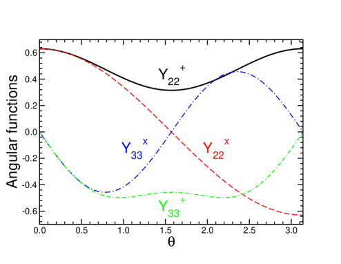
Let us now turn to the angular dependence of different multipolar components. From Eq. (16) we see that the relative amplitude of the modes is a complicated function of the sky position and orientation of the source, depending on products of the angular functions and . A possible way to determine the influence of these angles on the relative amplitude of the modes would be to perform Monte Carlo simulations, assuming random distributions for the angles. This is beyond the scope of this paper. Some insight can be obtained by plotting the -dependent combinations appearing in Eq. (16) (Fig. 3). For simplicity, let us consider the following two cases:
-
(i)
The angles are such that . Then the relative amplitude depends on the product of two factors: . In this case, from Fig. 3 we see that the “plus” component of the subdominant () multipole is never significantly enhanced with respect to the dominant multipole, because for all values of .
-
(ii)
The angles are such that . In this case the angular factor can blow up at the equator , so that the “subdominant” component will actually dominate the waveform for an observer located in this direction.
In conclusion, the relative amplitude is at most for non-spinning mergers with moderate mass ratios. Subdominant components can be amplified by the angular dependence of the radiation, but the likelihood of such an amplification should be quantified by a more detailed analysis. If the ratio of angular functions is of order unity, a relative amplitude can be thought of as a conservative estimate. From both point particle results and present-day simulations of spinning binaries in numerical relativity, we expect higher multipoles to be more excited for initially spinning black holes and large mass ratios. Below we illustrate the typical effect of subdominant multipoles on matched-filtering assuming .
Fitting factors and event loss due to single-mode templates
In our calculations of the FF we will assume that the angular dependence of the waveform (16) is such that the signal can be simplified to the form of Eq. (4). This assumption is not general enough. Our discussion above shows that it will only be valid for specific source locations in the sky, or for specific orientations of the detector: for example, the signal simplifies to Eq. (4) when or , as long as we consider an observer located at some constant and we appropriately define the azimuthal angles . A good strategy to address the general case could make use of Monte Carlo simulations. However, the simplified waveform (4) captures many of the important features we wish to address in this paper. Based on our discussion of the relative multipolar excitation we assume that mode “1” is the fundamental QNM with , and that mode “2” is the fundamental QNM with . We set the relative amplitude of the two modes , and to compute the QNM frequencies and quality factors we consider a dimensionless Kerr parameter (a typical value for the end-product of unequal-mass, non-spinning binary black hole mergers).
Fig. 1 shows Owen’s “minimal match” Owen:1995tm for this choice of parameters. The calculation is performed for different Earth-based detectors (LIGO, Virgo, Advanced LIGO and EGO) and the minimal match is computed as a function of the black hole’s mass in the source rest frame, . Thick lines assume that : roughly speaking, this means that the subdominant mode is “in phase” with the dominant multipole. Thin lines assume and , a rough way to simulate “dephased” signals. Intuitively we would expect a single-mode template to be a worse match for dephased signals. This expectation is confirmed by the fact that the minimal match is usually larger when (see below for a more detailed analysis). Values above the horizontal dashed line, corresponding to a , correspond to an event loss larger than . This illustrative calculation shows that, for the typical relative amplitudes expected from numerical relativity, single-mode templates can produce a significant event loss in Earth-based detectors when the black hole mass . This event loss can be fatal for detection of signals from very large mass IMBHs (), especially when the and components are not in phase. A more detailed discussion of the dependence of the FF on the phases ) can be found below.
 |
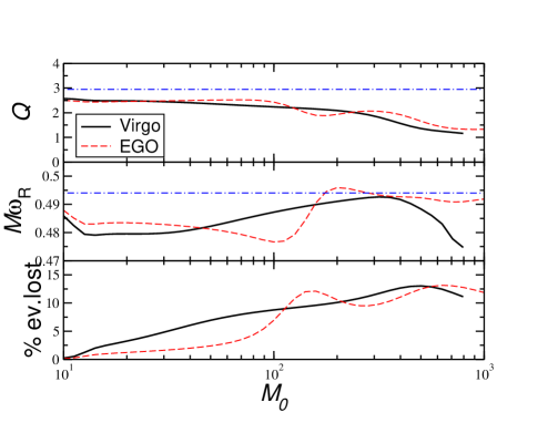 |
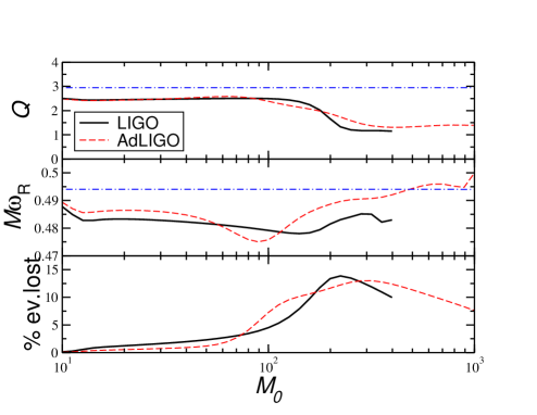
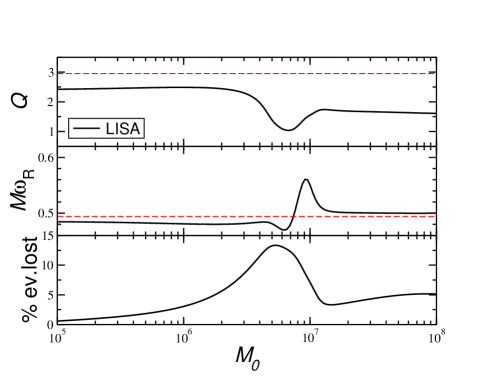
A low value of the FF is usually accompanied by a large bias in parameter estimation. This is illustrated quantitatively in Figs. 4 and 5, where we plot the quality factor and (dimensionless) frequency maximizing the FF, and the corresponding event loss, for different detectors. In Fig. 4 we consider Earth-based detectors of first and second generation. To be conservative, we perform the calculation in the “optimistic” case when the and modes start in phase (, ).
The QNM frequency of the dominant mode (horizontal dash-dotted line) is usually estimated with very good accuracy by a single-mode filter, except for very large values of the mass ( for LIGO and Virgo, and for second-generation detectors). Unfortunately, even when the FF is very high the single-mode filter produces a large bias in the quality factor of the dominant mode. For all Earth-based detectors we consider, this error is even for low values of the mass (), when the event loss is quite low and the filter works well for the purpose of detection. The bias on the quality factor gets even worse when we allow for a possible dephasing of the subdominant multipole (see Fig. 8 below). Being dimensionless, the quality factor of a QNM depends only on the dimensionless angular momentum of the black hole bcw . Therefore, a large bias in the quality factor means that single-mode templates cannot be used for accurate measurements of the black hole’s angular momentum, contrary to early claims in the literature (see e.g. Ref. echeverria ). Of course, this does not mean that such measurements are not possible. Single-mode templates are useful for detection (at least for small black hole masses), but multi-mode templates will be necessary if we want to perform precision measurements of a black hole’s properties using ringdown waves.
 |
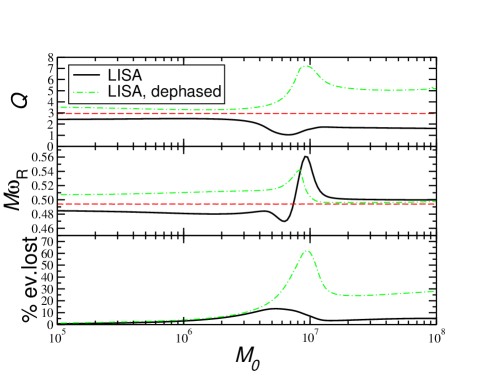 |
Fig. 5 shows that these remarks remain valid even for LISA, when the SNR is much larger and the detectable QNM frequencies much lower. In the plot we consider a source at Gpc (), for which the SNR can be bcw . The left panel shows the “optimistic” case when the first and second QNM signals are in phase. Even in this optimal situation the event loss can be as large as for masses , roughly the measured mass of the SMBH at the center of our own Galaxy. When the two QNM signals are dephased (green, dot-dashed line in the right panel) the event loss can be larger then for masses . Notice also that for , when the single-mode template works well for detection purposes, the bias on frequency and quality factor has opposite sign depending on whether the signals are in phase () or dephased (, ). This is no coincidence, as we will demonstrate below by studying the dependence of the bias on the phase angles .
Effect of the relative phase of the modes on detection and parameter estimation
So far we computed the FF assuming (so that the dominant QNM has maximum amplitude at ). We only explored the effect of the relative QNM phase by changing the sign333For , a sign change in is obviously equivalent to setting (what we referred to as the QNM signals being “in phase”) or (“dephased” signals), with an integer. of . In practice the situation is not so simple, since the phase of the two (or more) components of the “exact” signal is not known in advance. This problem is reminiscent of the analogous problem occurring in matched-filtering detection of inspiral signals (see Appendix B of Ref. Damour:1997ub ). For both inspiral and ringdown, maximizing the FF (8) over all parameters yields a “best possible overlap” which is somewhat optimistic, and therefore not too useful as a detectability criterion. More realistically, we should take into account our ignorance of the phase, or phases, of the “true” signal. This can be done by computing a “minimax” overlap Damour:1997ub : first maximize the FF (8) over all parameters of the template , and then minimize over the unknown phases of the actual inspiral or ringdown signal .
To discuss the difference between “best” and “minimax” overlaps in terms of detection and parameter estimation, here we perform FF calculations in the plane. We consider, for illustration, two cases:
-
(i)
An IMBH with as observed by LIGO;
-
(ii)
An IMBH with as observed by Advanced LIGO.
The FF for in these two cases is marked by a circle and a square, respectively, in Fig. 1. As in the rest of this Section, our signal will be given by the two-mode waveform (4) with and . This simple model is sufficient for our present purpose. A more detailed analysis (taking into account details of the angular dependence of the radiation, including a better model of the ringdown signal for spinning mergers, and possibly using waveforms from numerical relativity) is a topic for future work.
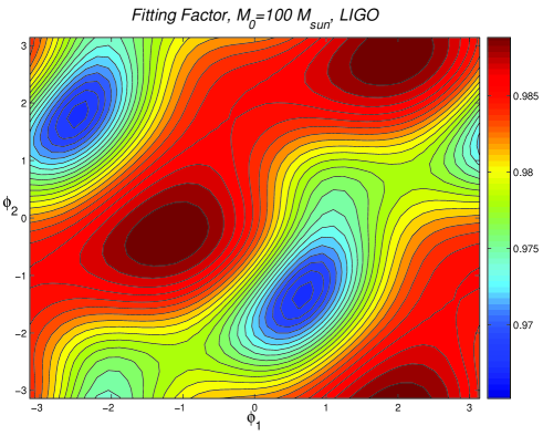
Fig. 6 shows a contour plot of the FF for case (i). The FF is always larger than , or equivalently, the event loss is always smaller than . For this particular system (and, presumably, for most low-mass black hole ringdowns) our ignorance of the phases does not sensibly reduce our chances of detecting the signal.
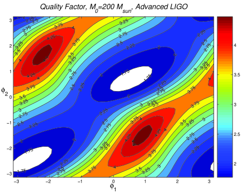
The plot shows interesting features, some of which are easy to understand. Under a simultaneous replacement , where are integers, the FF is unchanged. This is a trivial consequence of the fact that the overall sign of the signal (4) does not affect calculations of the FF. The FF has maxima and minima as a function of the two phases. Modulo periodicity, we see that the minimum occurs when and . This is reasonable: for these values of the phases the signals have comparable magnitude and opposite phase at , so that the multipole almost exactly cancels out the dominant multipole in the initial (and stronger) part of the signal. This destructive interference produces a signal that is sensibly different from a damped sinusoid, reducing the performance of a simple single-mode filter.
 |
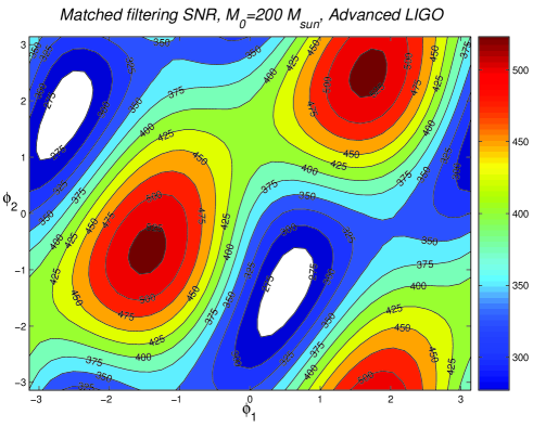 |
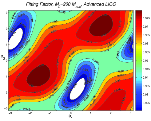
Fig. 7 shows contour plots of the FF and of the matched-filtering SNR , computed according to Eq. (9), for case (ii). Now the FF is smaller than in roughly half of the plane. The event loss ranges from to , being larger than in roughly half of the parameter space. From Fig. 1 we can expect that the event loss would have been even larger if we had chosen larger values of the black hole mass. The matched-filtering SNR was computed assuming that the overall amplitude of the signal corresponds to a ringdown efficiency , and that the luminosity distance Mpc. Both the FF and the SNR show the (by now familiar) -periodic pattern as a function of the phase angles.
 |
 |
Suppose that the event loss is moderately large but not so large to prevent a detection, as in case (ii). Then we may ask the question: what is the bias in measured parameters when maximize the probability of detection? In other words: when the template’s frequency and quality factor maximize the FF, do they also correspond to the “true” frequency and quality factor of the fundamental mode? Unfortunately, the answer is no.
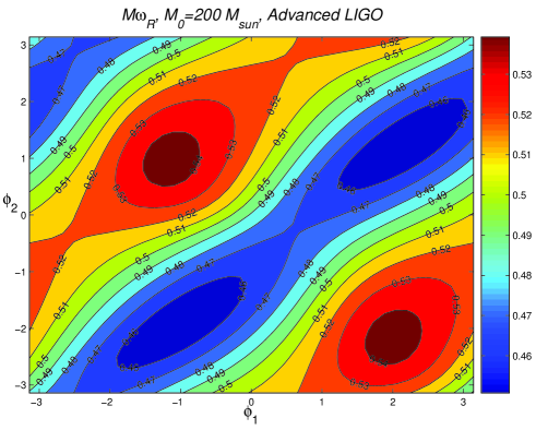
Fig. 8 shows the estimated dimensionless frequency (left) and quality factor (right) as functions of the phase angles. The estimated frequency has relatively small bias, and it always corresponds to the least-damped mode in the pair. Results are more interesting for the quality factor. For our chosen value of the Kerr parameter () the quality factor of the and modes are and , respectively. Comparing with Fig. 6, we see that relative minima in (and in the FF) occur when the quality factor “best fits” the mode. This is a rather remarkable result: the filter corresponding to the minimax overlap has a quality factor that “best fits” the subdominant mode in the pair. Unfortunately, maxima in do not correspond to the filter being optimally adapted to the mode. As the filter tries to maximize the overlap (and the SNR) the estimated value of the quality factor becomes significantly biased, and it deviates quite sensibly from the value expected from the dominant () mode. The bottom line is, once again, that single-mode filters can be useful for detection, but a multi-mode post-processing will be necessary for accurate measurements of the black hole’s angular momentum.
Another argument in favor of a two-stage search strategy comes from estimating the number of multi-mode templates that would be necessary for a detection. Searching for a larger number of modes implies a larger number of free parameters, and a correspondingly larger bank of filters. Matched-filtering requires that one covers the possible parameter space with a sufficiently fine template mesh, so that the best-matching template lies close enough to the true waveform. The distance between templates can be quantified in terms of a metric in template space, that was introduced by Owen Owen:1995tm following Refs. Sathyaprakash:1991mt ; Apostolatos:1995pj . If the mesh is too fine a very large number of templates may be required, a computationally expensive option. On the other hand, if the mesh is very coarse the template lying “closer” to the true waveform may produce a large event loss. A multi-mode search increases the number of templates needed for the mesh to be sufficiently fine. For a single-mode search, Creighton Creighton:1999pm estimated that templates are necessary to reduce the event loss below for LIGO and VIRGO. The same estimate can be used to show that templates would be necessary for single-mode templates with LISA Berti:2006ew . In Appendix A we estimate that the number of filters required for a two-mode template search would be much larger:
| (19) |
where is a factor of order unity which depends on the detector’s frequency span: with our choice of we get for LISA, EGO, Advanced LIGO, LIGO and Virgo, respectively. Using better template placing techniques nakano or imposing constraints on the functional form of the QNM frequencies (Appendix A) could help reduce computational requirements. A two-stage search seems to be a good compromise between performance and computational costs. Single-mode templates can be used for detection. Given a detection, multi-mode templates or Prony methods bcgs should be used for parameter estimation. A larger number of templates also means that the threshold for detection must be set higher, because there is a larger false alarm probability. Hierarchical searches or other techniques could play an important role in this regard reductionfalsealarm . In any case, such a large number of templates may not be a problem by the time advanced detectors are in operation. Improved computer performance and the use of large-scale computational projects, such as Einstein@Home einsteinathome , could be sufficient to overcome computational difficulties within the next decade.
IV Mode resolvability and no-hair tests
So far we looked at the event loss and bias in parameter estimation due to the use of single-mode templates to detect multi-mode signals. The discussion assumed that the gravitational wave signal is composed of at least two QNMs having roughly comparable amplitude. The question we address here is the following: how can we tell if there really are two or more modes in the signal, and can we resolve their parameters? If the noise is large and the amplitude of the weaker signal is very low, or the two signals have almost identical frequencies, the two modes could be difficult to resolve. This issue is particularly significant since no-hair tests using ringdown bcw require the presence and resolvability of two or more modes. Roughly speaking, the first mode is used to measure and by inverting the relations (see Appendix A for more details); the second mode can then be used to test consistency with the Kerr geometry.
Here we really address two different issues. We first assume that there are indeed two modes in the signal, and we discuss criteria to resolve their frequencies and damping times. This discussion parallels that in Ref. bcw , updating estimates of the relative mode excitation on the basis of recent results from numerical relativity, and correcting a typo in that paper. Then we introduce a rigorous criterion to resolve amplitudes: that is, we compute the minimum SNR such that one can decide by the presence of two modes in a given ringdown signal.
Resolving frequencies and damping times. A crude lower limit on the SNR required to resolve frequencies and damping times was presented in Ref. bcw . The analysis uses the statistical uncertainty in the determination of each frequency and damping time, which a standard Fisher Matrix calculation444Our Eq. (20a) corrects a missing factor of in Ref. bcw . estimates to be bcw
| (20a) | |||||
| (20b) | |||||
These errors refer to mode “1” in a pair. By considering the “symmetric” case , the errors on and are simply obtained by exchanging indices (). The expression above holds in both the FH and EF conventions, assuming white-noise for the detector, but modes “1” and “2” must correspond to different values of or (in the nomenclature used in Ref. bcw , the QNMs must be quasi-orthonormal).
A natural criterion (á la Rayleigh) to resolve frequencies and damping times is
| (21) |
In interferometry this would mean that two objects are (barely) resolvable if “the maximum of the diffraction pattern of object 1 is located at the minimum of the diffraction pattern of object 2”. We can introduce two “critical” SNRs required to resolve frequencies and damping times,
| (22) |
and recast our resolvability conditions as
| (23a) | |||||
| (23b) | |||||
The first condition implies resolvability of either the frequency or the damping time, the second implies resolvability of both.
Resolving amplitudes. A related question is: how large a SNR do we need to confidently say that we have detected a multi-mode signal, and to resolve two signals of different amplitudes? Suppose again, for simplicity, that the true signal is a two-mode superposition. Then we expect the weaker signal to be hard to resolve if its amplitude is low and the detector’s noise is large.
In Appendix B we quantify this statement by deriving a critical SNR for amplitude resolvability based on the generalized likelihood ratio test (GLRT), . The derivation of this critical SNR, which is given in Eq. (43), is based on the following simplifying assumptions: (i) using other criteria, we have already decided for the presence of one ringdown signal, and (ii) the parameters of the ringdown signal (frequencies and damping times), as well as the amplitude of the dominant mode, are known. In practice the latter assumption is not valid. For this reason, our estimates of the minimum SNR needed to detect more than one mode should be considered optimistic.
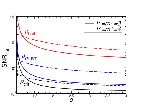
Fig. 9 compares the critical SNR , as defined in Eq. (43), and the two different criteria for frequency resolvability of Eq. (23). All quantities are computed as functions of the binary’s mass ratio . The angular momentum of the final black hole is computed using the fitting formula derived in Ref. Berti:2007fi for the angular momentum of the black hole resulting from unequal-mass, nonspinning binary black hole mergers: , where the symmetric mass ratio . This value of is then used to read QNM frequencies from numerical tables. We assume the dominant mode to be the fundamental QNM and for the subdominant mode we take the fundamental QNMs with or . To compute the relative amplitude for different mass ratios we use the EMOP estimate of Eq. (18a).
The plot shows that for all values of . Therefore, given a detection, the most important criterion to determine whether we can carry out no-hair tests seems to be the GLRT criterion. If we can decide for the presence of a second mode in the signal. Whenever the second mode is present, we also have : that is, we can resolve at least the frequencies (if not also the damping times) of the two modes. A SNR is typically enough to perform the GLRT test on the mode, as long as or so (equal-mass mergers should be quite rare anyway). By looking at Fig. 2 we conclude that not only LISA, but also advanced Earth-based detectors (Advanced LIGO and EGO) have the potential to identify Kerr black holes as the vacuum solutions of Einstein’s general relativity.
V Conclusions
In this paper we analyze the detectability of ringdown waves by Earth-based interferometers. Confirming and extending previous analyses, we show that Advanced LIGO and EGO could detect intermediate-mass black holes of mass up to out to a luminosity distance of a few Gpc.
Using recent results for the multipolar energy distribution from numerical relativity simulations of non-spinning binary black hole mergers Berti:2007fi to estimate the relative amplitude of the dominant multipolar components, we point out that the single-mode templates presently used for ringdown searches in the LIGO data stream could produce a significant event loss ( in a large interval of black hole masses). A similar event loss should affect also next-generation Earth-based detectors, as well as the planned space-based interferometer LISA.
Single-mode templates are useful for detection of low-mass systems, but they produce large errors in the estimated values of the parameters (and especially of the quality factor). We estimate that, unfortunately, more than templates would be needed for a single-stage multi-mode search. For this reason we recommend a “two stage” search to save on computational costs: a single-mode template could be used to detect the signal, and a multi-mode template (or even better, Prony methods bcgs ) could be used to estimate parameters once a detection has been made.
In Appendix B we introduce a criterion to decide for the presence of more than one mode in a ringdown signal. By updating estimates of the critical signal-to-noise ratio required to resolve the frequencies of different QNMs using results from numerical relativity, we show that second-generation Earth-based detectors and LISA both have the potential to perform tests of the Kerr nature of astrophysical black holes.
In the future we plan to use numerical waveforms (possibly including spin effects) to refine our estimates. We also plan to carry out Monte Carlo simulations to study the information that can be extracted on the source position and orientation using a network of Earth-based detectors. The possibility to constrain the black hole spin’s direction from the multipolar distribution of the merger-ringdown radiation should be particularly interesting (eg. for coincident electromagnetic observations of jets that could be emitted along the black hole spin’s axis).
Acknowledgements
We are grateful to Alessandra Buonanno, Kostas Kokkotas, Clifford Will and Nicolas Yunes for discussions. This work was partially funded by Fundação para a Ciência e Tecnologia (FCT) - Portugal through projects PTDC/FIS/64175/2006 and POCI/FP/81915/2007, by the National Science Foundation under grant numbers PHY 03-53180 and PHY 06-52448, and by NASA under grant number NNG06GI60 to Washington University.
Appendix A Number of templates for a two-mode search
Two-mode ringdown waveforms of the form (4) depend of five parameters: two quality factors , two frequencies and one relative amplitude between the different modes (for simplicity, here we set ). For matched-filtering with ringdown waveforms of unknown frequency and quality factor we must lay down a “mesh” covering the parameter space with some pre-defined precision (that can be translated to a pre-defined minimum loss of SNR) Sathyaprakash:1991mt ; Owen:1995tm ; Creighton:1999pm . We follow Owen’s formalism Owen:1995tm to estimate the necessary number of templates. The distance between nearby templates, which defines the mismatch between the filters, can be computed in terms of the metric
| (24) |
where (for large or moderate values of and ) the metric coefficients are well approximated by
| (25a) | |||||
| (25b) | |||||
| (25c) | |||||
| (25d) | |||||
| (25e) | |||||
| (25f) | |||||
| (25g) | |||||
| (25h) | |||||
Requiring a loss of no more than in the event rate due to a mismatched template (i.e, the minimal match MM Owen:1995tm ; Creighton:1999pm should be at least ) we get an estimate for the number of templates we need:
| (26) |
Here is a factor of order unity which depends on the detector’s frequency span. We get for LISA, EGO, Advanced LIGO, LIGO and Virgo, respectively. In deriving this number we assume the frequencies to be searched for are those of interest for each of the detectors ( for LISA, for EGO, for Advanced LIGO and Virgo, for LIGO), that the quality factor varies between and for all modes likely to be detected bcw , and that the relative amplitude varies between and . Our estimates are not strongly sensitive to the relative amplitude: assuming yields a total number of templates which is roughly half the above number.
For the single-mode case, setting we get the following metric:
| (27) |
The number of templates Creighton:1999pm . In particular we get for LIGO and Virgo Creighton:1999pm , and for LISA Berti:2006ew (a huge improvement in terms of computational requirements).
The formalism and numbers presented in this section are valid for a general ringdown signal: no constraints were imposed on the QNM spectrum. A possible approach to reduce the number of templates is to assume that the source is a general relativistic black hole. In this case, we are left with only three intrinsic parameters: the mass and angular momentum of the black hole and the relative amplitude between the modes. Alternatively, we can choose the independent parameters to be one quality factor , one frequency and the relative amplitude of the modes; the quality factor and frequency of the second mode, and , can be thought of as functions of and .
More explicitly, we find that for rotations the frequencies and quality factors of the fundamental mode with are well approximated (to within or better) by
| (28) | |||||
| (29) |
By inverting these relations for (say) the mode, one can infer and compute the frequency and quality factor of the modes with . More generally, in Ref. bcw the frequencies and quality factors of the first three overtones (for and all values of ) were fitted by functions of the form
| (30) | |||||
| (31) |
Here the constants and depend on (see Tables VIII-X in bcw ), and the fits are accurate to better than . By using these fits or (more precisely) numerical QNM data we can express any subdominant mode in terms of the dominant mode, and possibly reduce the number of templates.
Another possibility to reduce the number of templates is to restrict the parameter space by using information derived from measurements of the inspiral waveforms. For example, if we had a reasonably accurate measurement of the masses and spins of the binary members we could significantly restrict the possible values of the mass and spin of the final black hole to be searched for.
Appendix B Amplitude resolvability
The purpose of this Appendix is to estimate the minimum SNR required to test the hypothesis that a second mode is present in a ringdown waveform. The derivation is based on the following simplifying assumptions: (i) using other criteria, we have already decided for the presence of one (dominant) damped sinusoid in the signal, and (ii) the parameters of the ringdown signal (frequencies and damping times), as well as the amplitude of the dominant mode, are known. In practice the latter assumption is not valid, so our estimates of the minimum SNR should be considered optimistic.
The question of whether one or two damped sinusoids are present in the signal can be stated in statistical terms, as follows555See also the work by Milanfar and Shahram smilanfar ; milanfars .. Let be a zero-mean gaussian white noise process, and define to be the difference between the actual signal and the dominant normalized QNM signal (for simplicity, in the present discussion we set ). Denote by the hypothesis that the signal contains only one damped exponential in noise, and by the hypothesis that the signal consists of two damped exponentials in noise:
| (32) |
We write the normalized second QNM as .
We assume that we do not possess any prior information on the possible values of , besides the fact that . The general structure of composite hypothesis testing is involved when unknown parameters (in this case, ) appear in the probability density function. We follow Milanfar and Shahram smilanfar ; milanfars and consider the generalized likelihood ratio test, which proceeds by computing first the maximum likelihood (ML) estimates of the unknown parameters. These estimates are then used to form Neyman-Pearson detectors. We note that this approach has been compared very favorably against other standard tests in Ref. smilanfar .
Suppose that the signal is sampled at discrete times and that the corresponding sample values are . If we assume additive white noise with variance , the probability of the observed data under the hypothesis of a second damped sinusoid of amplitude in the signal is
| (33) |
To decide on hypothesis or , we start by computing the ML estimate of the unknown parameter :
| (34) |
where Y and are column-vectors of the samples and , respectively, a superscript stands for “transpose”, and denotes the norm of a vector V. The (unconstrained) ML estimate of the parameter is then
| (35) |
We wish to test the hypothesis that against the hypothesis that . There is no general-purpose test to do this, but a powerful test is to compute a likelihood ratio and to find the maximum in both the numerator and denominator: this is called the generalized likelihood ratio test (GLRT). Some algebra shows that
| (36) |
For any given data set Y, we decide on if exceeds a specified threshold :
| (37) |
While it may seem troublesome to use the unconstrained ML estimate to form the GLRT, in fact, due to the assumed positivity of , the detector structure is effectively producing a one-sided test and therefore this is in fact a uniformly most powerful detector Scharf1991 .
The choice of is motivated by the level of tolerable false-positive rate smilanfar ; milanfars . The detection rate and false alarm rate for this detector are related as
| (38) |
where
| (39) |
Here denotes the right-tail probability function for a standard Gaussian random variable (zero mean and unit variance):
| (40) |
From (38) we find
| (41) |
This last expression can now be put in a more convenient form, by defining the output SNR as
| (42) |
Using (39) and (41) the relation between the minimum resolvable and the required SNR can be made explicit. The critical SNR for hypothesis testing is
| (43) |
For the calculations in Fig. 9 we set , . Had we chosen and , the critical would have decreased by a factor . For more stringent false alarm rates (say, with and ) the critical SNR would have increased by a factor .
References
- (1) R. Narayan, New J. Phys. 7, 199 (2005) [arXiv:gr-qc/0506078].
- (2) J. P. Lasota, Comptes Rendus Physique 8, 45 (2007) [arXiv:astro-ph/0607453].
- (3) S. A. Hughes, In the Proceedings of 33rd SLAC Summer Institute on Particle Physics (SSI 2005): Gravity in the Quantum World and the Cosmos, Menlo Park, California, 25 Jul - 5 Aug 2005, pp L006 [arXiv:hep-ph/0511217].
- (4) K. D. Kokkotas and B. G. Schmidt, Living Rev. Rel. 2, 2 (1999); H. -P. Nollert, Class. Quant. Grav. 16, R159 (1999).
- (5) E. Berti, V. Cardoso and C. M. Will, Phys. Rev. D 73, 064030 (2006) [arXiv:gr-qc/0512160].
- (6) F. Echeverria, Phys. Rev. D 40, 3194 (1989).
- (7) L. S. Finn, Phys. Rev. D 46, 5236 (1992).
- (8) E. E. Flanagan and S. A. Hughes, Phys. Rev. D 57, 4535 (1998).
- (9) O. Dreyer, B. Kelly, B. Krishnan, L. S. Finn, D. Garrison and R. Lopez-Aleman, Class. Quant. Grav. 21, 787 (2004) [arXiv:gr-qc/0309007].
- (10) E. Berti, V. Cardoso, J. A. Gonzalez, U. Sperhake, M. Hannam, S. Husa and B. Bruegmann, arXiv:gr-qc/0703053.
- (11) M. Luna and A. M. Sintes, Class. Quant. Grav. 23, 3763 (2006) [arXiv:gr-qc/0601072].
- (12) C. Cutler and K. S. Thorne, arXiv:gr-qc/0204090.
- (13) J. S. B. Wyithe and A. Loeb, Astrophys. J. 612, 597 (2004) [arXiv:astro-ph/0312080].
- (14) K. Belczynski, T. Bulik and B. Rudak, Astrophys. J. 608, L45 (2004) [arXiv:astro-ph/0403361].
- (15) K. Kulczycki, T. Bulik, K. Belczynski and B. Rudak, arXiv:astro-ph/0602533.
- (16) J. M. Fregeau, S. L. Larson, M. C. Miller, R. O’Shaughnessy and F. A. Rasio, Astrophys. J. 646, L135 (2006) [arXiv:astro-ph/0605732].
- (17) A. Buonanno, G. B. Cook and F. Pretorius, arXiv:gr-qc/0610122.
- (18) J. G. Baker, S. T. McWilliams, J. R. van Meter, J. Centrella, D. I. Choi, B. J. Kelly and M. Koppitz, Phys. Rev. D 75, 124024 (2007) [arXiv:gr-qc/0612117].
- (19) Y. Pan et al., arXiv:0704.1964 [gr-qc].
- (20) P. Ajith et al., arXiv:0704.3764 [gr-qc].
- (21) I. Mandel, D. A. Brown, J. R. Gair and M. C. Miller, arXiv:0705.0285 [astro-ph].
- (22) L. M. Goggin (for the LIGO Scientific Collaboration), Class. Quant. Grav. 23, S709 (2006).
- (23) J. Clark, I. S. Heng, M. Pitkin and G. Woan, arXiv:gr-qc/0703138.
- (24) B. J. Owen, Phys. Rev. D 53, 6749 (1996).
- (25) H. Nakano, H. Takahashi, H. Tagoshi and M. Sasaki, Phys. Rev. D 68, 102003 (2003); idem, Progr. Theor. Phys. 111, 781 (2004); Y. Tsunesada et al., Phys. Rev. D 71, 103005 (2005) [arXiv:gr-qc/0410037]; Y. Tsunesada, D. Tatsumi, N. Kanda and H. Nakano [TAMA Collaboration], Class. Quant. Grav. 22, S1129 (2005).
- (26) K. Ioka and H. Nakano, arXiv:0704.3467 [astro-ph].
- (27) T. A. Apostolatos, Phys. Rev. D 52, 605 (1995).
- (28) T. Damour, B. R. Iyer and B. S. Sathyaprakash, Phys. Rev. D 63, 044023 (2001) [Erratum-ibid. D 72, 029902 (2005)].
- (29) http://www.ligo.caltech.edu/advLIGO/scripts/ref_des.shtml
- (30) C. Van Den Broeck and A. S. Sengupta, Class. Quant. Grav. 24, 155 (2007).
- (31) E. Berti, A. Buonanno and C. M. Will, Phys. Rev. D 71, 084025 (2005) [arXiv:gr-qc/0411129].
- (32) E. Berti, V. Cardoso, J. A. Gonzalez and U. Sperhake, arXiv:gr-qc/0701086.
- (33) A. Pai, C. Celsi, G. V. Pallottino, S. D’Antonio and P. Astone, Class. Quant. Grav. 24, 1457 (2007).
- (34) J. G. Baker, J. R. van Meter, S. T. McWilliams, J. Centrella and B. J. Kelly, arXiv:gr-qc/0612024.
- (35) W. H. Press, S. A. Teukolsky, W. T. Vetterling and B. P. Flannery, Numerical Recipes in Fortran, Second Edition (Cambridge University Press, Cambridge, 1992).
- (36) E. Berti, V. Cardoso and M. Casals, Phys. Rev. D 73, 024013 (2006) [Erratum-ibid. D 73, 109902 (2006)] [arXiv:gr-qc/0511111].
- (37) K. S. Thorne, in 300 Years of Gravitation, Ed. S. W. Hawking and W. Israel (Cambridge University Press, Cambridge, 1987).
- (38) T. Damour, B. R. Iyer and B. S. Sathyaprakash, Phys. Rev. D 57, 885 (1998) [arXiv:gr-qc/9708034].
- (39) B. S. Sathyaprakash and S. V. Dhurandhar, Phys. Rev. D 44, 3819 (1991); S. V. Dhurandhar and B. S. Sathyaprakash, Phys. Rev. D 49, 1707 (1994).
- (40) J. D. E. Creighton, Phys. Rev. D 60, 022001 (1999).
- (41) E. Berti, Class. Quant. Grav. 23, S785 (2006).
- (42) S. D. Mohanty and S. V. Dhurandhar, Phys. Rev. D 54, 7108 (1996); S. Mitra, S. V. Dhurandhar and L. S. Finn, Phys. Rev. D 72, 102001 (2005).
- (43) http://einstein.phys.uwm.edu/
- (44) M. Shahram and P. Milanfar, IEEE Transactions on Signal Processing 53, 2579 (2005).
- (45) P. Milanfar and A. Shakouri, Proceedings of the International Conference on Image Processing, 864-867 (2002); M. Shahram and P. Milanfar, Digital Signal Processing 15, 305 (2005).
- (46) L. L. Scharf, “Statistical Signal Processing, Detection, Estimation, and Time Series Analysis,” (Addison-Wesley, Reading, MA, 1991).