Model-independent constraints on $\mathbf{\Delta F=2}$ operators
and the scale of New Physics

Abstract

We update the constraints on new-physics contributions to $\Delta F=2$ processes from the generalized unitarity triangle analysis, including the most recent experimental developments. Based on these constraints, we derive upper bounds on the coefficients of the most general $\Delta F=2$ effective Hamiltonian. These upper bounds can be translated into lower bounds on the scale of new physics that contributes to these low-energy effective interactions. We point out that, due to the enhancement in the renormalization group evolution and in the matrix elements, the coefficients of non-standard operators are much more constrained than the coefficient of the operator present in the Standard Model. Therefore, the scale of new physics in models that generate new $\Delta F=2$ operators, such as next-to-minimal flavour violation, has to be much higher than the scale of minimal flavour violation, and it most probably lies beyond the reach of direct searches at the LHC.

I Introduction

Starting from the pioneering measurements of the $K^{0}-\bar{K}^{0}$ mass difference $\Delta m_{K}$ and of the CP-violating parameter $\varepsilon_{K}$, continuing with the precision measurements of the $B_{d}-\bar{B}_{d}$ mixing parameters $\Delta m_{B_{d}}$ and $\sin 2\beta$ and with the recent determination of the $B_{s}-\bar{B}_{s}$ oscillation frequency $\Delta m_{B_{s}}$ and the first bounds on the mixing phase $-2\beta_{s}$, until the very recent evidence of $D^{0}-\bar{D}^{0}$ mixing, $\Delta F=2$ processes have always provided some of the most stringent constraints on New Physics (NP).

For example, it has been known for more than a quarter of century that supersymmetric extensions of the Standard Model (SM) with generic flavour structures are strongly constrained by $K^{0}-\bar{K}^{0}$ mixing and CP violation susyjurassic . The constraints from $K^{0}-\bar{K}^{0}$ mixing are particularly stringent for models that generate transitions between quarks of different chiralities LRjurassic ; pellicanino ; pellicani . More recently, it has been shown that another source of enhancement of chirality-breaking transitions lies in the QCD corrections bagger , now known at the Next-to-Leading Order (NLO) NLOgen ; BBSUSY .

Previous phenomenological analyses of $\Delta F=2$ processes in supersymmetry SUSYKKbar ; SUSYBBbar were affected by a large uncertainty due to the SM contribution, since no determination of the Cabibbo-Kobayashi-Maskawa ckm (CKM) CP-violating phase was available in the presence of NP. A breakthrough was possible with the advent of $B$ factories and the measurement of time-dependent CP asymmetries in $B$ decays, allowing for a simultaneous determination of the CKM parameters and of the NP contributions to $\Delta F=2$ processes in the $K^{0}$ and $B_{d}$ sectors UTfitNP05 ; UTfitNP06 ; othernp . Furthermore, the Tevatron experiments have provided the first measurement of $\Delta m_{B_{s}}$ and the first bounds on the phase of $B_{s}-\bar{B}_{s}$ mixing. Combining all these ingredients, we can now determine allowed ranges for all NP $\Delta F=2$ amplitudes in the down-quark sector.

To complete the picture, the recent evidence of $D^{0}-\bar{D}^{0}$ mixing allows to constrain NP contributions to the $\Delta C=2$ amplitude noiddbar ; altriddbar .

Our aim in this work is to consider the most general effective Hamiltonian for $\Delta F=2$ processes ($\mathcal{H}_{\mathrm{eff}}^{\Delta F=2}$) and to translate the experimental constraints into allowed ranges for the Wilson coefficients of $\mathcal{H}_{\mathrm{eff}}^{\Delta F=2}$. These coefficients in general have the form

$$C_{i}(\Lambda)=\frac{F_{i}L_{i}}{\Lambda^{2}}\,$$ (1)

where $F_{i}$ is a function of the (complex) NP flavour couplings, $L_{i}$ is a loop factor that is present in models with no tree-level Flavour Changing Neutral Currents (FCNC), and $\Lambda$ is the scale of NP, i.e. the typical mass of the new particles mediating $\Delta F=2$ transitions. For a generic strongly-interacting theory with arbitrary flavour structure, one expects $F_{i}\sim L_{i}\sim 1$ so that the allowed range for each of the $C_{i}(\Lambda)$ can be immediately translated into a lower bound on $\Lambda$. Specific assumptions on the flavour structure of NP, for example Minimal mfv ; uut ; dambrosio or Next-to-Minimal papucci Flavour Violation (MFV or NMFV), correspond to particular choices of the $F_{i}$ functions, as detailed below.

Our study is analogous to the operator analysis of electroweak precision observables barbierietal , but it provides much more stringent bounds on models with non-minimal flavour violation. In particular, we find that the scale of heavy particles mediating tree-level FCNC in models of NMFV must lie above $\sim 60$ TeV, making them undetectable at the LHC. This bound applies for instance to the Kaluza-Klein excitations of gauge bosons in a large class of models with (warped) extra dimensions soni . Flavour physics remains the main avenue to probe such extensions of the SM.

The paper is organised as follows. In Sec. II we briefly discuss the experimental novelties considered in our analysis. In Sec. III we present updated results for the analysis of the Unitarity Triangle (UT) in the presence of NP, including the model-independent constraints on $\Delta F=2$ processes, following closely our previous analyses UTfitNP05 ; UTfitNP06 . In Sec. IV we discuss the structure of $\mathcal{H}_{\mathrm{eff}}^{\Delta F=2}$, the definition of the models we consider and the method used to constrain the Wilson coefficients. In Sec. V we present our results for the Wilson coefficients and for the scale of NP. Conclusions are drawn in Sec. VI.

II Experimental input

We use the same experimental input as Ref. UTfitNP06 , updated after the Winter ${}^{\prime}07$ conferences. We collect all the numbers used throughout this paper in Tables 1 and 2. We include the following novelties: the most recent result for $\Delta m_{s}$ dmsCDF , the semileptonic asymmetry in $B_{s}$ decays $A_{\mathrm{SL}}^{s}$ ASLD0 and the dimuon charge asymmetry $A_{\mathrm{SL}}^{\mu\mu}$ from D$\O$ ACHD0 and CDF ASLCDF , the measurement of the $B_{s}$ lifetime from flavour-specific final states tauBsflavspec , the determination of $\Delta\Gamma_{s}/\Gamma_{s}$ from the time-integrated angular analysis of $B_{s}\to J/\psi\phi$ decays by CDF DGoGCDF , the three-dimensional constraint on $\Gamma_{s}$, $\Delta\Gamma_{s}$, and the phase $\phi_{s}$ of the $B_{s}$–$\bar{B}_{s}$ mixing amplitude from the time-dependent angular analysis of $B_{s}\to J/\psi\phi$ decays by D$\O$ DGoGD0 .

Parameter	Value	Gaussian ($\sigma$)	Uniform
			(half-width)
$\lambda$	0.2258	0.0014	-
$\left|V_{cb}\right|\times 10^{3}$(excl.)	$39.1$	$0.6$	$1.7$
$\left|V_{cb}\right|\times 10^{3}$(incl.)	$41.7$	$0.7$	-
$\left|V_{ub}\right|\times 10^{4}$(excl.)	$34$	$4$	-
$\left|V_{ub}\right|\times 10^{4}$(incl.)	$43.1$	$3.9$	-
$\Delta m_{d}$ (ps-1)	$0.507$	$0.005$	-
$\Delta m_{s}$ (ps-1)	$17.77$	$0.12$	-
$\epsilon_{K}\times 10^{3}$	$2.232$	$0.007$	-
$\sin 2\beta$	see Winter ’07 analysis at http://www.utfit.org
$\cos 2\beta$	see Winter ’07 analysis at http://www.utfit.org
$\alpha$	see Winter ’07 analysis at http://www.utfit.org
$\gamma$	see Winter ’07 analysis at http://www.utfit.org
$2\beta+\gamma$	see Winter ’07 analysis at http://www.utfit.org
$\overline{m}_{t}$ (GeV)	$161.2$	$1.7$	-
$\alpha_{s}(M_{Z})$	0.119	0.003	-
$\tau_{B_{s}}$ (ps)	1.39	0.12	-
$\tau_{B_{s}}^{FS}$ (ps)	1.454	0.040	-
$A_{\mathrm{SL}}^{d}$	-0.0005	0.0056	-
$A_{\mathrm{SL}}^{s}$	0.0245	0.0196	-
$A_{\mathrm{SL}}^{\mu\mu}$	-0.0043	0.0030	-
$\Delta\Gamma_{d}/\Gamma_{d}$	0.009	0.037	-
$\Delta\Gamma_{s}/\Gamma_{s}$	0.65	0.33	-
$\phi_{s}$ [rad]	-0.79	0.56	$\phi_{s}$-$\tau_{B_{s}}$ corr. 0.727
$\tau_{B_{s}}$ (ps)	1.49	0.08	$\tau_{B_{s}}$-$\Delta\Gamma_{s}/\Gamma_{s}$ corr. -0.172
$\Delta\Gamma_{s}/\Gamma_{s}$	0.17	0.09	$\Delta\Gamma_{s}/\Gamma_{s}$-$\phi_{s}$ corr. -0.188

Table 1: Values of the experimental input used in our analysis. The Gaussian and the flat contributions to the uncertainty are given in the third and fourth columns respectively (for details on the statistical treatment see noi ). See text for details.

Parameter	Value	Gaussian ($\sigma$)	Uniform
			(half-width)
$F_{D}$ (MeV)	$201$	$3$	$17$
$F_{B_{s}}\sqrt{B_{s}}$ (MeV)	$262$	$35$	-
$\xi=\frac{F_{B_{s}}\sqrt{B_{s}}}{F_{B_{d}}\sqrt{B_{d}}}$	1.23	0.06	-
$\hat{B}_{K}$	0.79	0.04	0.08
$\overline{m}_{b}$ (GeV)	4.21	0.08	-
$\overline{m}_{c}$ (GeV)	1.3	0.1	-
$R_{1}$	1	-	-
$R_{2}$	-12.9	3.0	-
$R_{3}$	3.98	0.89	-
$R_{4}$	20.8	4.4	-
$R_{5}$	5.2	1.2	-
$B_{1}^{D}$	0.865	0.02	0.015
$B_{2}^{D}$	0.82	0.03	0.01
$B_{3}^{D}$	1.07	0.05	0.08
$B_{4}^{D}$	1.08	0.02	0.02
$B_{5}^{D}$	1.455	0.03	0.075
$B_{1}^{B}$	0.88	0.04	0.10
$B_{2}^{B}$	0.82	0.03	0.09
$B_{3}^{B}$	1.02	0.06	0.13
$B_{4}^{B}$	1.15	0.03	0.13
$B_{5}^{B}$	1.99	0.04	0.24

Table 2: Values of the hadronic parameters used in our analysis. The Gaussian and the flat contributions to the uncertainty are given in the third and fourth columns respectively (for details on the statistical treatment see noi ). See the text for details.

The use of $\Delta\Gamma_{s}/\Gamma_{s}$, from the time-integrated angular analysis of $B_{s}\to J/\psi\phi$ decays, is described in Ref. UTfitNP06 . In this paper, we only use the CDF measurement as input, since the D$\O$ analysis is now superseded by the new time-dependent study. The latter provides the first direct constraint on the $B_{s}$–$\bar{B}_{s}$ mixing phase, but also a simultaneous bound on $\Delta\Gamma_{s}$ and $\Gamma_{s}$. We implemented the full $3\times 3$ correlation matrix. The time-dependent analysis determines the $B_{s}$–$\bar{B}_{s}$ mixing phase with a four-fold ambiguity.  First of all, the $B_{s}$ mesons are untagged, so the analysis is not directly sensitive to $\sin\phi_{s}$, resulting in the ambiguity $(\phi_{s},\cos\delta_{1,2})\leftrightarrow(-\phi_{s},-\cos\delta_{1,2})$, where $\delta_{1,2}$ represent the strong phase differences between the transverse polarization and the other ones. Second, at fixed sign of $\cos\delta_{1,2}$, there is the ambiguity $(\phi_{s},\Delta\Gamma_{s})\leftrightarrow(\phi_{s}+\pi,-\Delta\Gamma_{s})$. Concerning the strong phases $\delta_{i}$, there is a two-fold ambiguity corresponding to $\delta_{i}\to\pi-\delta_{i}$. The two experimental determinations are roughly $\delta_{2}\sim 0$, $\delta_{1}\sim\pi$ and $\delta_{1}\sim 0$, $\delta_{2}\sim\pi$. In the literature it is often found that factorization corresponds to the first choice dighe ; digheold ; nierste . However, we find that factorization predicts $\delta_{1}\sim 0$, $\delta_{2}\sim\pi$ kramer ; neubert ; beneke . This result is also compatible with the BaBar measurement in $B\to J/\Psi K^{*}$ babarjpsikst , which can be related to $B_{s}\to J/\Psi\phi$ using $SU(3)$ and neglecting singlet contributions. However, waiting for future, more sophisticated experimental analyses which could resolve this ambiguity, we prefer to be conservative and keep the four-fold ambiguity in our analysis.

The use of $\Delta m_{s}$ was already discussed in Ref. UTfitNP06 . The only difference with respect to that is the update of the experimental inputs: we now use the improved measurement by CDF dmsCDF , and we take $\tau_{B_{s}}$ only from the study of $B_{s}$ decays to CP eigenstates tauBsCP . The value of $\tau_{B_{s}}$ obtained from $B_{s}$ decaying to flavour-specific final states, using a single exponential in the fit, is related to the values of $\Gamma_{s}$ and $\Delta\Gamma_{s}$ by the relation teoTauBs

$$\tau_{B_{s}}^{FS}=\frac{1}{\Gamma_{s}}\frac{1+\left(\frac{\Delta\Gamma_{s}}{2\Gamma_{s}}\right)^{2}}{1-\left(\frac{\Delta\Gamma_{s}}{2\Gamma_{s}}\right)^{2}}\,,$$ (2)

which provides an independent constraint on $\Delta\Gamma_{s}/\Gamma_{s}$. We compute $\Delta\Gamma_{s}$ and $A_{\mathrm{SL}}^{s}$ using eq. (7) of Ref. UTfitNP06 (recalling that $A_{\mathrm{SL}}^{s}=2(1-|q/p|_{s})$. Following Ref. nir , we use the value of $A_{\mathrm{SL}}^{\mu\mu}$ recently presented by D$\O$ ACHD0 and CDF ASLCDF , in the form

$$A_{\mathrm{SL}}^{\mu\mu}=\frac{f_{d}\chi_{d0}A_{\mathrm{SL}}^{d}+f_{s}\chi_{s0}A_{\mathrm{SL}}^{s}}{f_{d}\chi_{d0}+f_{s}\chi_{s0}}\,,$$ (3)

with $f_{d}=0.397\pm 0.010$, $f_{s}=0.107\pm 0.011$, $\chi_{q0}=(\chi_{q}+\bar{\chi}_{q})/2$. $\chi_{q}$ and $\bar{\chi}_{q}$ are computed using equations (3)-(5) of Ref. UTfitNP06 .

Finally, concerning $D^{0}-\bar{D}^{0}$ mixing, we use as input the results for the NP amplitude obtained in Ref. noiddbar combining the experimental information from Refs. ddbarexp .

III UT analysis and constraints on NP

The contribution of NP to $\Delta F=2$ transitions can be parameterized in a model-independent way as the ratio of the full (SM+NP) amplitude to the SM one. In this way, we can define the parameters $C_{B_{q}}$ and $\phi_{B_{q}}$ ($q=d,\,s$) as cfactors :

$$C_{B_{q}}\,e^{2i\phi_{B_{q}}}=\frac{\langle B_{q}|H_{\mathrm{eff}}^{\mathrm{full}}|\bar{B}_{q}\rangle}{\langle B_{q}|H_{\mathrm{eff}}^{\mathrm{SM}}|\bar{B}_{q}\rangle}\,,$$ (4)

and write all the measured observables as a function of these parameters and the SM ones ($\bar{\rho}$, $\bar{\eta}$, and additional parameters such as masses, form factors, and decay constants). Details are given in Refs. UTfitNP05 ; UTfitNP06 . In a similar way, one can write

$$C_{\epsilon_{K}}=\frac{\mathrm{Im}[\langle K^{0}|H_{\mathrm{eff}}^{\mathrm{full}}|\bar{K}^{0}\rangle]}{\mathrm{Im}[\langle K^{0}|H_{\mathrm{eff}}^{\mathrm{SM}}|\bar{K}^{0}\rangle]}\,,\qquad C_{\Delta m_{K}}=\frac{\mathrm{Re}[\langle K^{0}|H_{\mathrm{eff}}^{\mathrm{full}}|\bar{K}^{0}\rangle]}{\mathrm{Re}[\langle K^{0}|H_{\mathrm{eff}}^{\mathrm{SM}}|\bar{K}^{0}\rangle]}\,.$$ (5)

Concerning $\Delta m_{K}$, to be conservative, we add to the short-distance contribution a possible long-distance one that varies with a uniform distribution between zero and the experimental value of $\Delta m_{K}$.

Figure 1: Determination of $\bar{\rho}$ and $\bar{\eta}$ from the NP generalized analysis. $68\%$ and $95\%$ probability regions for $\bar{\rho}$ and $\bar{\eta}$ are shown, together with the $2\,\sigma$ contours given by the tree-level determination of $|V_{ub}|$ and $\gamma$.

Parameter	$68\%$ Probability	$95\%$ Probability
$C_{B_{d}}$	$1.05\pm 0.34$	$[0.53,2.05]$
$\phi_{B_{d}}[^{\circ}]$	$-3.4\pm 2.2$	$[-8.3,1.6]$
$C_{B_{s}}$	$1.11\pm 0.32$	$[0.63,2.07]$
$\phi_{B_{s}}[^{\circ}]$	$(-69\pm 14)$ $\cup$ $(-20\pm 14)$ $\cup$ $(20\pm 5)$ $\cup$ $(72\pm 8)$	$[-86,-46]$ $\cup$ $[-43,35]$ $\cup$ $[56,87]$
$C_{\Delta m_{K}}$	$0.93\pm 0.32$	$[0.51,2.07]$
$C_{\epsilon_{K}}$	$0.92\pm 0.14$	$[0.66,1.31]$
$\overline{\rho}$	$0.140\pm 0.046$	$[0.049,0.258]$
$\overline{\eta}$	$0.384\pm 0.035$	$[0.304,0.460]$
$\alpha[^{\circ}]$	$86\pm 7$	$[73,104]$
$\beta[^{\circ}]$	$24.3\pm 2.0$	$[19.9,28.6]$
$\gamma[^{\circ}]$	$70\pm 7$	$[53,83]$
$\rm{Re}{\lambda}_{t}$[$10^{-5}$]	$-31.3\pm 1.8$	$[-35,-27]$
$\rm{Im}{\lambda}_{t}$[$10^{-5}$]	$14.8\pm 1.3$	$[12.3,17.3]$
$|V_{ub}|[10^{-3}]$	$3.91\pm 0.28$	$[3.36,4.44]$
$|V_{cb}|[10^{-2}]$	$4.09\pm 0.05$	$[3.98,4.18]$
$|V_{td}|[10^{-3}]$	$8.7\pm 0.5$	$[7.6,9.6]$
$|V_{td}/V_{ts}|$	$0.217\pm 0.012$	$[0.187,0.240]$
$R_{b}$	$0.413\pm 0.030$	$[0.354,0.471]$
$R_{t}$	$0.943\pm 0.048$	$[0.819,1.037]$
$\sin 2\beta$	$0.748\pm 0.044$	$[0.643,0.841]$
$\sin 2\beta_{s}$	$0.0409\pm 0.0038$	$[0.0321,0.0494]$

Table 3: Determination of NP and UT parameters from the UT fit.

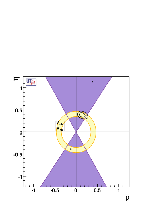
We perform a global analysis using the method of Ref. noi and determine simultaneously $\bar{\rho}$, $\bar{\eta}$, $C_{B_{q}}$, $\phi_{B_{q}}$, $C_{\epsilon_{K}}$ and $C_{\Delta m_{K}}$ using flat a-priori distributions for these parameters. The resulting probability density function (p.d.f.) in the $\bar{\rho}-\bar{\eta}$ plane is shown in Fig. 1. Only a small region close to the result of the SM fit survives. The mirror solution in the third quadrant is suppressed down to about $5\%$ probability by the measurements of $A_{\mathrm{SL}}^{d}$ and $A_{\mathrm{SL}}^{\mu\mu}$. The results for $\bar{\rho}$ and $\bar{\eta}$ reported in Tab. 3 are at a level of accuracy comparable to the SM fit UTfitSM06 , so that the SM contribution to FCNC processes in the presence of arbitrary NP is bound to lie very close to the results of the SM in the absence of NP. This result represents a major improvement in the study of FCNC processes beyond the SM, and opens up the possibility of precision studies of flavour processes in the presence of NP.

Figure 2: Constraints on $\phi_{B_{d}}$ vs. $C_{B_{d}}$, $\phi_{B_{s}}$ vs. $C_{B_{s}}$ and $C_{\epsilon_{K}}$ vs $C_{\Delta m_{K}}$ from the NP generalized analysis.

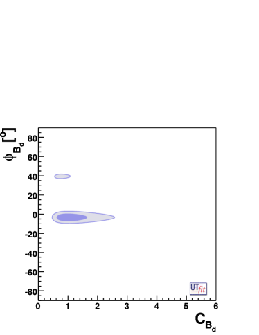
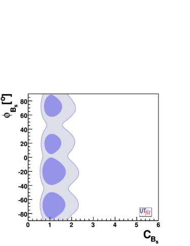
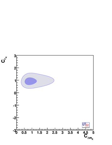
The constraining power of this analysis is evident in the results for the NP parameters given in Tab. 3 and shown in Fig. 2. Compared to our previous analysis in Ref. UTfitNP06 , and to similar analyses in the literature otherBs ; nir , we see that the additional experimental input discussed above improves considerably the determination of the phase of the $B_{s}-\bar{B}_{s}$ mixing amplitude. The fourfold ambiguity inherent in the untagged analysis of Ref. DGoGD0 is somewhat reduced by the measurements of $A_{\mathrm{SL}}^{s}$ and $A_{\mathrm{SL}}^{\mu\mu}$, which prefer negative values of $\phi_{B_{s}}$. Ref. nierste recently claimed a $2\sigma$ deviation from zero in $\phi_{B_{s}}$, taking the sign of $\cos\delta_{1,2}$ from factorization. We confirm that, with the same assumptions of Ref. nierste on strong phases, the deviation from zero of $\phi_{B_{s}}$ slightly exceeds $2\sigma$. Without assuming strong phases from factorization, we find a deviation of $\phi_{B_{s}}$ from zero of $1.4~{}\sigma$, of the same size of the deviation found experimentally by Ref. DGoGD0 .

It is important to stress that the information contained in these constraints does not rely on any specific model for NP. The list of applications in NP phenomenology is rich. For instance, restricting to the case of SUSY models, the two-dimensional constraint of the $b\to s$ ($b\to d$) sector can be translated into a limit on the mass-insertion complex parameters $\delta^{d}_{23}$ ($\delta^{d}_{13}$), using the NLO supersymmetric expression of the $B_{q}$–$\bar{B}_{q}$ mixing amplitude BBSUSY . This bound, combined with the constraint from $b\to s$ decays massinsertion , allows to obtain the best available information on the off-diagonal terms of the squark mass matrix valentina . However, in the following, rather than considering an explicit model for NP, we perform a general analysis based on the most general Hamiltonian for $\Delta F=2$ processes.

IV NP contributions to $\mathbf{\Delta F=2}$ processes

The most general effective Hamiltonians for $\Delta F=2$ processes beyond the SM have the following form:

$${\cal H}_{\rm eff}^{\Delta S=2}=\sum_{i=1}^{5}C_{i}\,Q_{i}^{sd}+\sum_{i=1}^{3}\tilde{C}_{i}\,\tilde{Q}_{i}^{sd}$$ (6)

$${\cal H}_{\rm eff}^{\Delta C=2}=\sum_{i=1}^{5}C_{i}\,Q_{i}^{cu}+\sum_{i=1}^{3}\tilde{C}_{i}\,\tilde{Q}_{i}^{cu}$$

$${\cal H}_{\rm eff}^{\Delta B=2}=\sum_{i=1}^{5}C_{i}\,Q_{i}^{bq}+\sum_{i=1}^{3}\tilde{C}_{i}\,\tilde{Q}_{i}^{bq}$$

where $q=d(s)$ for $B_{d(s)}-\bar{B}_{d(s)}$ mixing and

$$Q_{1}^{q_{i}q_{j}} = \bar{q}^{\alpha}_{jL}\gamma_{\mu}q^{\alpha}_{iL}\bar{q}^{\beta}_{jL}\gamma^{\mu}q^{\beta}_{iL}\;,$$

$$Q_{2}^{q_{i}q_{j}} = \bar{q}^{\alpha}_{jR}q^{\alpha}_{iL}\bar{q}^{\beta}_{jR}q^{\beta}_{iL}\;,$$

$$Q_{3}^{q_{i}q_{j}} = \bar{q}^{\alpha}_{jR}q^{\beta}_{iL}\bar{q}^{\beta}_{jR}q^{\alpha}_{iL}\;,$$ (7)

$$Q_{4}^{q_{i}q_{j}} = \bar{q}^{\alpha}_{jR}q^{\alpha}_{iL}\bar{q}^{\beta}_{jL}q^{\beta}_{iR}\;,$$

$$Q_{5}^{q_{i}q_{j}} = \bar{q}^{\alpha}_{jR}q^{\beta}_{iL}\bar{q}^{\beta}_{jL}q^{\alpha}_{iR}\;.$$

Here $q_{R,L}=P_{R,L}\,q$, with $P_{R,L}=(1\pm\gamma_{5})/2$, and $\alpha$ and $\beta$ are colour indices. The operators $\tilde{Q}_{1,2,3}^{q_{i}q_{j}}$ are obtained from the $Q_{1,2,3}^{q_{i}q_{j}}$ by the exchange $L\leftrightarrow R$. In the following we only discuss the operators $Q_{i}$ as the results for $Q_{1,2,3}$ apply to $\tilde{Q}_{1,2,3}$ as well.

The NLO anomalous dimension matrix has been computed in NLOgen . We use the Regularisation-Independent anomalous dimension matrix in the Landau gauge (also known as RI-MOM), since this scheme is used in lattice QCD calculations of the matrix elements with non-perturbative renormalization.

The $C_{i}(\Lambda)$ are obtained by integrating out all new particles simultaneously at the NP scale $\Lambda$. We then have to evolve the coefficients down to the hadronic scales $\mu_{b}=m_{b}=4.6$ GeV ($m_{b}\equiv m_{b}(\mu=m_{b})$ is the RI-MOM mass) for bottom mesons, $\mu_{D}=2.8$ GeV for charmed mesons, and $\mu_{K}=2$ GeV for Kaons, which are the renormalisation scales of the operators used in lattice computations for the matrix elements bpark ; hep-lat/0110091 .

We give here an analytic formula for the contribution to the $B_{q}-\bar{B}_{q}$ mixing amplitudes induced by a given NP scale coefficient $C_{i}(\Lambda)$, denoted by $\langle\bar{B}_{q}|{\cal H}_{\rm eff}|B_{q}\rangle_{i}$, as a function of $\alpha_{s}(\Lambda)$:

$$\langle\bar{B}_{q}|{\cal H}_{\rm eff}^{\Delta B=2}|B_{q}\rangle_{i}=\sum_{j=1}^{5}\sum_{r=1}^{5}\left(b^{(r,i)}_{j}+\eta\,c^{(r,i)}_{j}\right)\eta^{a_{j}}\,C_{i}(\Lambda)\,\langle\bar{B}_{q}|Q_{r}^{bq}|B_{q}\rangle\,,$$ (8)

where $\eta=\alpha_{s}(\Lambda)/\alpha_{s}(m_{t})$, the magic numbers $a_{j}$, $b^{(r,i)}_{j}$ and $c^{(r,i)}_{j}$ and the matrix elements can be found in eqs. (10) and (12) of Ref. SUSYBBbar respectively. The values of the $B^{B}_{i}$ parameters can be found in Table 2. A similar formula holds for $D^{0}-\bar{D}^{0}$ mixing, with the parameters $B^{D}_{i}$ given in Table 2 and the following magic numbers:

$$\begin{array}[]{l l}a_{i}=(0.286,-0.692,0.787,-1.143,0.143)&\\ &\\ b^{(11)}_{i}=(0.837,0,0,0,0),&c^{(11)}_{i}=(-0.016,0,0,0,0),\\ b^{(22)}_{i}=(0,2.163,0.012,0,0),&c^{(22)}_{i}=(0,-0.20,-0.002,0,0),\\ b^{(23)}_{i}=(0,-0.567,0.176,0,0),&c^{(23)}_{i}=(0,-0.016,0.006,0,0),\\ b^{(32)}_{i}=(0,-0.032,0.031,0,0),&c^{(32)}_{i}=(0,0.004,-0.010,0,0),\\ b^{(33)}_{i}=(0,0.008,0.474,0,0),&c^{(33)}_{i}=(0,0.000,0.025,0,0),\\ b^{(44)}_{i}=(0,0,0,3.63,0),&c^{(44)}_{i}=(0,0,0,-0.56,0.006),\\ b^{(45)}_{i}=(0,0,0,1.21,-0.19),&c^{(45)}_{i}=(0,0,0,-0.29,-0.006),\\ b^{(54)}_{i}=(0,0,0,0.14,0),&c^{(54)}_{i}=(0,0,0,-0.019,-0.016),\\ b^{(55)}_{i}=(0,0,0,0.045,0.839),&c^{(55)}_{i}=(0,0,0,-0.009,0.018).\\ \end{array}$$ (9)

All other magic numbers vanish. Finally, for $K^{0}-\bar{K}^{0}$ mixing we obtain

$$\langle\bar{K}^{0}|{\cal H}_{\rm eff}^{\Delta S=2}|K^{0}\rangle_{i}=\sum_{j=1}^{5}\sum_{r=1}^{5}\left(b^{(r,i)}_{j}+\eta\,c^{(r,i)}_{j}\right)\eta^{a_{j}}\,C_{i}(\Lambda)\,R_{r}\,\langle\bar{K}^{0}|Q_{1}^{sd}|K^{0}\rangle\,,$$ (10)

where now the magic numbers can be found in eq. (2.7) of Ref. SUSYKKbar . We use the values in Table 2 for the ratios $R_{r}$ of the matrix elements of the NP operators $Q_{r}^{sd}$ over the SM one. These values correspond to the average of the results in Ref. bpark , applying a scaling factor to the errors to take into account the spread of the available results.

To obtain the p.d.f. for the Wilson coefficients at the NP scale $\Lambda$, we switch on one coefficient at a time in each sector and calculate its value from the result of the NP analysis presented in sec. III.

As we discussed in eq. (1), the connection between the $C_{i}(\Lambda)$ and the NP scale $\Lambda$ depends on the general properties of the NP model, and in particular on the flavour structure of the $F_{i}$. Assuming strongly interacting new particles, we have from eq. (1) with $L_{i}=1$

$$\Lambda=\sqrt{\frac{F_{i}}{C_{i}}}\,.$$ (11)

Let us now discuss four notable examples:

• In the case of MFV with one Higgs doublet or two Higgs doublets with small or moderate $\tan\beta$, we have $F_{1}=F_{\mathrm{SM}}$ and $F_{i\neq 1}=0$, where $F_{\mathrm{SM}}$ is the combination of CKM matrix elements appearing in the top-quark mediated SM mixing amplitude, namely $(V_{tq}V_{tb}^{*})^{2}$ for $B_{q}-\bar{B}_{q}$ mixing and $(V_{td}V_{ts}^{*})^{2}$ for $\varepsilon_{K}$. $\Delta m_{K}$ and $D^{0}-\bar{D}^{0}$ mixing do not give significant constraints in this scenario due to the presence of long-distance contributions.

• In the case of MFV at large $\tan\beta$, we have this additional contribution to $B_{q}-\bar{B}_{q}$ mixing dambrosio :

  $$C_{4}(\Lambda)=\frac{(a_{0}+a_{1})(a_{0}+a_{2})}{\Lambda^{2}}\lambda_{b}\lambda_{q}F_{\mathrm{SM}}\,,$$ (12)

  where $\lambda_{b,q}$ represent the corresponding Yukawa couplings, $a_{0,1,2}$ are $\tan\beta$-enhanced loop factors of $\mathcal{O}(1)$ and $\Lambda$ represents the NP scale corresponding to the non-standard Higgs bosons.

• In the case of NMFV, we have $|F_{i}|=F_{\mathrm{SM}}$ with an arbitrary phase papucci (following Ref. dambrosio , for $\Delta m_{K}$ and $D^{0}-\bar{D}^{0}$ mixing we take $F_{\mathrm{SM}}=|V_{td}V_{ts}|^{2}$). This condition is realized in models in which right-handed currents also contribute to FCNC processes, but with the same hierarchical structure in the mixing angles as in the SM left-handed currents. Given the order-of-magnitude equalities $m_{d}/m_{b}\sim|V_{td}|$, $m_{s}/m_{b}\sim|V_{ts}|$, bounds obtained in this scenario are also of interest for extra-dimensional models with FCNC couplings suppressed linearly with quark masses soni . Clearly, given the QCD and, for $K^{0}-\bar{K}^{0}$ mixing, chiral enhancement of NP operators, the constraints on the NP scale are much stronger for NMFV than for MFV, as shown explicitly in the next section.

• For arbitrary NP flavour structures, we expect $|F_{i}|\sim 1$ with arbitrary phase. In this case, the constraints on the NP scale are much tighter due to the absence of the CKM suppression in the NP contributions.

V Results

In this Section, we present the results obtained for the four scenarios described above. In deriving the lower bounds on the NP scale $\Lambda$, we assume $L_{i}=1$, corresponding to strongly-interacting and/or tree-level NP. Two other interesting possibilities are given by loop-mediated NP contributions proportional to $\alpha_{s}^{2}$ or $\alpha_{W}^{2}$. The first case corresponds for example to gluino exchange in the MSSM. The second case applies to all models of SM-like loop-mediated weak interactions. To obtain the lower bound on $\Lambda$ for loop-mediated contributions, one simply multiplies the bounds we quote in the following by $\alpha_{s}(\Lambda)\sim 0.1$ or by $\alpha_{W}\sim 0.03$.

Let us first consider MFV models and update our results presented in Ref. UTfitNP05 ; UTfitNP06 . In practice, the most convenient strategy in this case is to fit the shift in the Inami-Lim top-quark function entering $B_{d}$, $B_{s}$ and $K^{0}$ mixing. We fit for this shift using the experimental measurements of $\Delta m_{d}$, $\Delta m_{s}$ and $\epsilon_{K}$, after determining the parameters of the CKM matrix with the universal unitarity triangle analysis uut . We obtain the following lower bounds at $95\%$ probability:

$$\Lambda>5.5\,\mathrm{TeV}\quad\mathrm{(small}\,\tan\beta\mathrm{)}\,,$$ (13)

$$\Lambda>5.1\,\mathrm{TeV}\quad\mathrm{(large}\,\tan\beta\mathrm{)}\,.$$ (14)

The bound for large $\tan\beta$ comes from contributions proportional to the same operator present in the SM.

As mentioned above, at very large $\tan\beta$ additional contributions to $C_{4}(\Lambda)$ can be generated by Higgs exchange. From these contributions, we obtain the following lower bound on the scale $\Lambda$, which in this case is the mass of non-standard Higgs bosons:

$$M_{H}>5\,\sqrt{(a_{0}+a_{1})(a_{0}+a_{2})}\left(\frac{\tan\beta}{50}\right)\,\mathrm{TeV}\,.$$ (15)

In any given model, one can specify the value of the $a_{i}$ couplings and of $\tan\beta$ to obtain a lower bound on the non-standard Higgs mass. The bound we obtained is in agreement with Ref. dambrosio , taking into account the present experimental information. If a non-standard Higgs boson is seen at hadron colliders, this implies an upper bound on the $a_{i}$ couplings and/or $\tan\beta$.

Figure 3: Allowed ranges in the Re$C^{i}_{K}$-Im$C^{i}_{K}$ planes in GeV^-2. Light (dark) regions correspond to $95\%$ ($68\%$) probability regions.

Figure 4: Allowed ranges in the Abs$C^{i}_{D}$-Arg$C^{i}_{D}$ planes in GeV^-2. Light (dark) regions correspond to $95\%$ ($68\%$) probability regions.

Figure 5: Allowed ranges in the Abs$C^{i}_{B_{d}}$-Arg$C^{i}_{B_{d}}$ planes in GeV^-2. Light (dark) regions correspond to $95\%$ ($68\%$) probability regions.

Figure 6: Allowed ranges in the Abs$C^{i}_{B_{s}}$-Arg$C^{i}_{B_{s}}$ planes in GeV^-2. Light (dark) regions correspond to $95\%$ ($68\%$) probability regions.

Parameter	$95\%$ allowed range	Lower limit on $\Lambda$ (TeV)	Lower limit on $\Lambda$ (TeV)
	(GeV-2)	for arbitrary NP	for NMFV
Re$C_{K}^{1}$	$[-9.6,9.6]\cdot 10^{-13}$	$1.0\cdot 10^{3}$	$0.35$
Re$C_{K}^{2}$	$[-1.8,1.9]\cdot 10^{-14}$	$7.3\cdot 10^{3}$	$2.0$
Re$C_{K}^{3}$	$[-6.0,5.6]\cdot 10^{-14}$	$4.1\cdot 10^{3}$	$1.1$
Re$C_{K}^{4}$	$[-3.6,3.6]\cdot 10^{-15}$	$17\cdot 10^{3}$	$4.0$
Re$C_{K}^{5}$	$[-1.0,1.0]\cdot 10^{-14}$	$10\cdot 10^{3}$	$2.4$
Im$C_{K}^{1}$	$[-4.4,2.8]\cdot 10^{-15}$	$1.5\cdot 10^{4}$	$5.6$
Im$C_{K}^{2}$	$[-5.1,9.3]\cdot 10^{-17}$	$10\cdot 10^{4}$	$28$
Im$C_{K}^{3}$	$[-3.1,1.7]\cdot 10^{-16}$	$5.7\cdot 10^{4}$	$19$
Im$C_{K}^{4}$	$[-1.8,0.9]\cdot 10^{-17}$	$24\cdot 10^{4}$	$62$
Im$C_{K}^{5}$	$[-5.2,2.8]\cdot 10^{-17}$	$14\cdot 10^{4}$	$37$
$|C_{D}^{1}|$	$<7.2\cdot 10^{-13}$	$1.2\cdot 10^{3}$	$0.40$
$|C_{D}^{2}|$	$<1.6\cdot 10^{-13}$	$2.5\cdot 10^{3}$	$0.82$
$|C_{D}^{3}|$	$<3.9\cdot 10^{-12}$	$0.51\cdot 10^{3}$	$0.17$
$|C_{D}^{4}|$	$<4.8\cdot 10^{-14}$	$4.6\cdot 10^{3}$	$1.5$
$|C_{D}^{5}|$	$<4.8\cdot 10^{-13}$	$1.4\cdot 10^{3}$	$0.47$
$|C_{B_{d}}^{1}|$	$<2.3\cdot 10^{-11}$	$0.21\cdot 10^{3}$	$1.8$
$|C_{B_{d}}^{2}|$	$<7.2\cdot 10^{-13}$	$1.2\cdot 10^{3}$	$8.5$
$|C_{B_{d}}^{3}|$	$<2.8\cdot 10^{-12}$	$0.60\cdot 10^{3}$	$4.4$
$|C_{B_{d}}^{4}|$	$<2.1\cdot 10^{-13}$	$2.2\cdot 10^{3}$	$14$
$|C_{B_{d}}^{5}|$	$<6.0\cdot 10^{-13}$	$1.3\cdot 10^{3}$	$8.8$
$|C_{B_{s}}^{1}|$	$<1.1\cdot 10^{-9}$	$30$	$1.3$
$|C_{B_{s}}^{2}|$	$<5.6\cdot 10^{-11}$	$130$	$4.6$
$|C_{B_{s}}^{3}|$	$<2.1\cdot 10^{-10}$	$70$	$2.4$
$|C_{B_{s}}^{4}|$	$<1.6\cdot 10^{-11}$	$250$	$7.9$
$|C_{B_{s}}^{5}|$	$<4.5\cdot 10^{-11}$	$150$	$4.9$

Table 4: $95\%$ probability range for $C(\Lambda)$ and the corresponding lower bounds on the NP scale $\Lambda$ for arbitrary NP flavour structure and for NMFV. See the text for details.

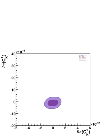
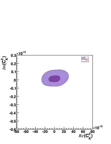
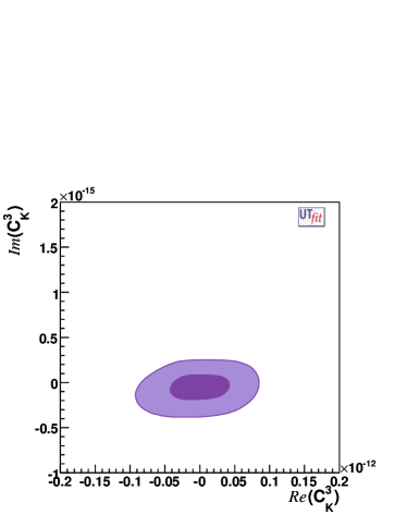
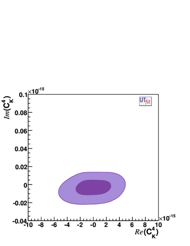
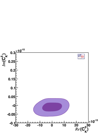
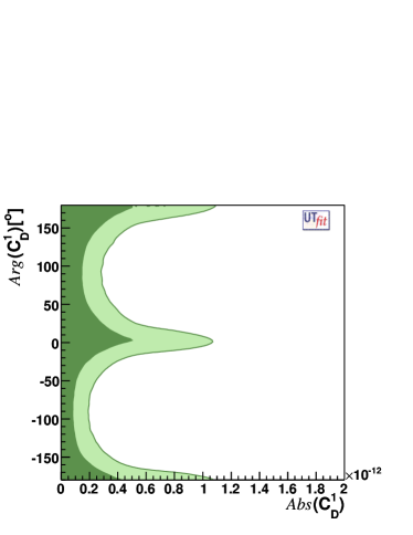
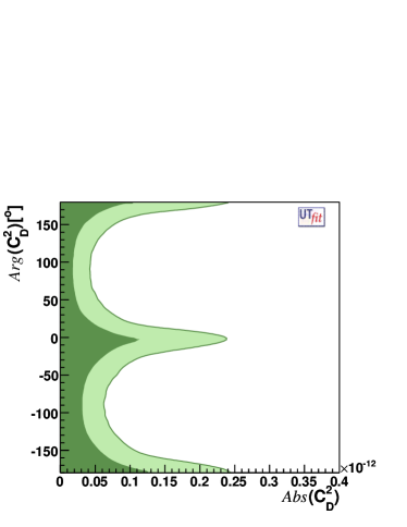
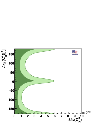
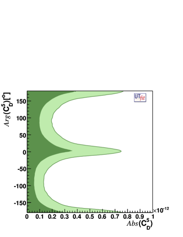
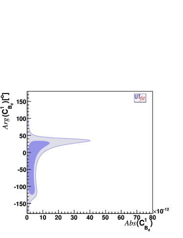
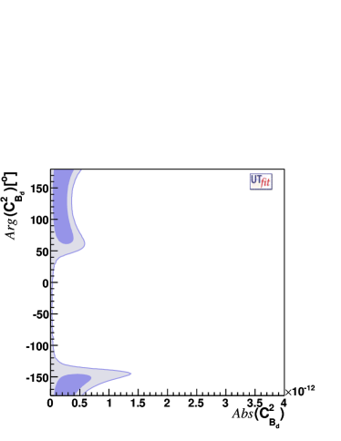
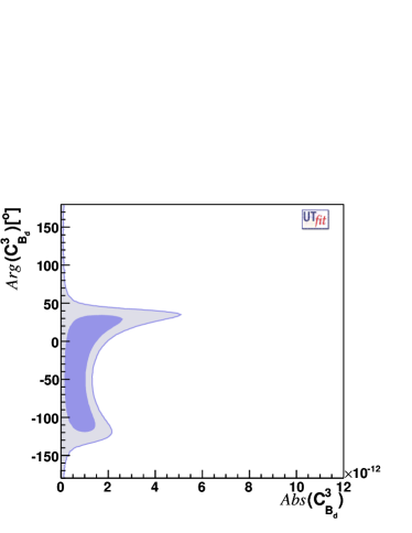
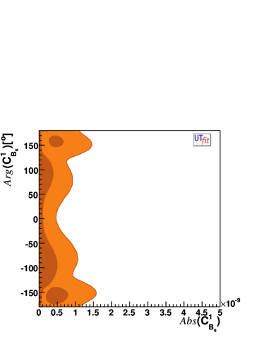
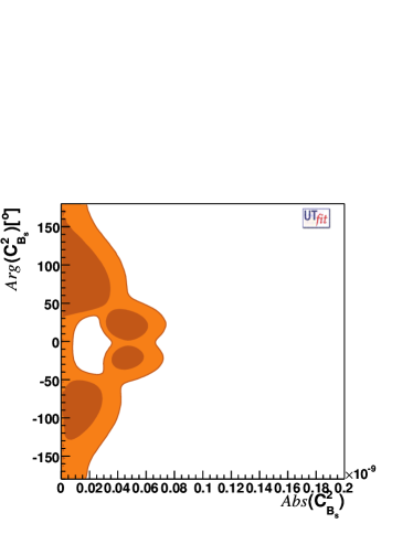
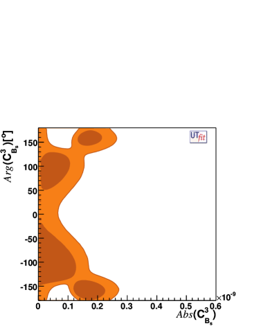
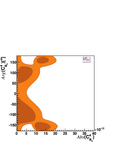
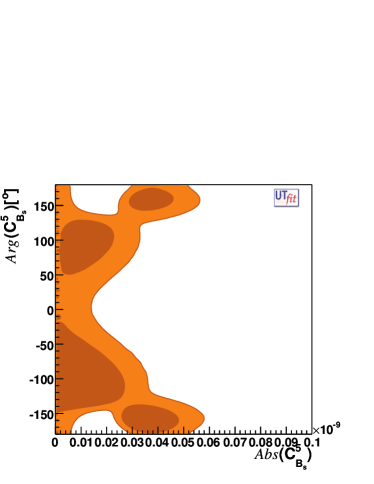
In Fig. 3 we present the allowed regions in the Re$C^{i}$-Im$C^{i}$ planes for the $K^{0}$ sector, while in Figs. 4-6 we show the allowed regions in the Abs$C^{i}$-Arg$C^{i}$ planes for the $D^{0}$, $B_{d}$ and $B_{s}$ sectors. All coefficients are given in GeV^-2. From these allowed regions we obtain the $95\%$ probability regions for $C^{i}$ reported in the second column of Tab. 4. This result is completely model-independent.

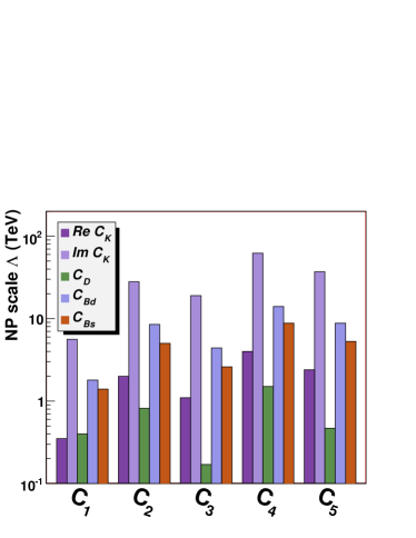
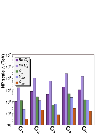
Assuming strongly interacting and/or tree-level NP contributions with generic flavour structure (i.e. $L_{i}=|F_{i}|=1$), we can translate the upper bounds on $C_{i}$ into the lower bounds on the NP scale $\Lambda$ reported in the third column of Tab. 4. As anticipated above, we see that in the $K^{0}$ sector all bounds from non-standard operators are one order of magnitude stronger than the bound from the SM operator, due to the chiral enhancement. In addition, operator $Q_{4}$ has the strongest Renormalization Group (RG) enhancement. In the $D^{0}$, $B_{d}$ and $B_{s}$ sectors, the chiral enhancement is absent, but the RG enhancement is still effective. The overall constraint on the NP scale $\Lambda$ comes from Im$C^{4}_{K}$ and reads, for strongly interacting and/or tree-level NP, $\alpha_{s}$ loop mediated or $\alpha_{W}$ loop mediated respectively:

$$\Lambda^{\mathrm{GEN}}_{\mathrm{tree}}>2.4\cdot 10^{5}\,\mathrm{TeV},\quad\Lambda^{\mathrm{GEN}}_{\mathrm{\alpha_{s}}}>2.4\cdot 10^{4}\,\mathrm{TeV},\quad\Lambda^{\mathrm{GEN}}_{\mathrm{\alpha_{W}}}>8\cdot 10^{3}\,\mathrm{TeV}.$$ (16)

Assuming strongly interacting and/or tree-level NP contributions with NMFV flavour structure (i.e. $L_{i}=1$ and $|F_{i}|=|F_{\mathrm{SM}}|$), we can translate the upper bounds on $C_{i}$ into the lower bounds on the NP scale $\Lambda$ reported in the fourth column of Tab. 4. The flavour structure of NMFV models implies that the bounds from the four sectors are all comparable, the strongest one being obtained from Im$C^{4}_{K}$ (barring, as always, accidental cancellations):

$$\Lambda^{\mathrm{NMFV}}_{\mathrm{tree}}>62\,\mathrm{TeV},\quad\Lambda^{\mathrm{NMFV}}_{\mathrm{\alpha_{s}}}>6.2\,\mathrm{TeV},\quad\Lambda^{\mathrm{NMFV}}_{\mathrm{\alpha_{W}}}>2\,\mathrm{TeV}.$$ (17)

Let us now comment on the possibility of direct detection of NP at LHC, given the bounds we obtained. Clearly, a loop suppression is needed in all scenarios to obtain NP scales that can be reached at the LHC. For NMFV models, an $\alpha_{W}$ loop suppression might not be sufficient, since the resulting NP scale is $2$ TeV. Of course, if there is an accidental suppression of the NP contribution to $\epsilon_{K}$, the scale for weak loop contributions might be as low as $0.5$ TeV. The general model is out of reach even for $\alpha_{W}$ (or stronger) loop suppression. For MFV models at large values of $\tan\beta$, stringent constraints on the mass of the non-standard Higgs bosons can be obtained. These particles may or may not be detectable at the LHC depending on the actual value of $\tan\beta$. Finally, the reader should keep in mind the possibility of accidental cancellations among the contribution of different operators, which might weaken the bounds we obtained.

VI Conclusions

We have presented bounds on the NP scale $\Lambda$ obtained from an operator analysis of $\Delta F=2$ processes, using the most recent experimental measurements, the NLO formulae for the RG evolution and the Lattice QCD results for the matrix elements. We have considered four scenarios: MFV at small $\tan\beta$, MFV at large $\tan\beta$, NMFV and general NP with arbitrary flavour structure. The lower bounds on the scale $\Lambda$ of strongly-interacting NP for NMFV and general NP scenarios (barring accidental cancellations) are reported in Fig. 7. Taking the most stringent bound for each scenario, we obtain the bounds given in Table 5.

Figure 7: Summary of the $95\%$ probability lower bound on the NP scale $\Lambda$ for strongly-interacting NP in NMFV (left) and general NP (right) scenarios.

Scenario	strong/tree	$\alpha_{s}$ loop	$\alpha_{W}$ loop
MFV (small $\tan\beta$)	5.5	0.5	0.2
MFV (large $\tan\beta$)	5.1	0.5	0.2
$M_{H}$ in MFV at large $\tan\beta$	$5\,\sqrt{(a_{0}+a_{1})(a_{0}+a_{2})}\left(\frac{\tan\beta}{50}\right)\,$
NMFV	62	6.2	2
General	24000	2400	800

Table 5: Summary of the $95\%$ probability lower bound on the NP scale $\Lambda$ (in TeV) for several possible flavour structures and loop suppressions.

We conclude that any model with strongly interacting NP and/or tree-level contributions is beyond the reach of direct searches at the LHC. Flavour and CP violation remain the main tool to constrain (or detect) such NP models. Weakly-interacting extensions of the SM can be accessible at the LHC provided that they enjoy a MFV-like suppression of $\Delta F=2$ processes, or at least a NMFV-like suppression with an additional depletion of the NP contribution to $\epsilon_{K}$.

References

- (1) J. R. Ellis and D. V. Nanopoulos, Phys. Lett. B 110 (1982) 44; J. F. Donoghue, H. P. Nilles and D. Wyler, Phys. Lett. B 128 (1983) 55; J. M. Frere and M. Belen Gavela, Phys. Lett. B 132 (1983) 107; M. J. Duncan and J. Trampetic, Phys. Lett. B 134 (1984) 439; J. M. Gerard, W. Grimus, A. Raychaudhuri and G. Zoupanos, Phys. Lett. B 140 (1984) 349; J. M. Gerard, W. Grimus and A. Raychaudhuri, Phys. Lett. B 145 (1984) 400; J. M. Gerard, W. Grimus, A. Masiero, D. V. Nanopoulos and A. Raychaudhuri, Nucl. Phys. B 253 (1985) 93.
- (2) G. Beall, M. Bander and A. Soni, Phys. Rev. Lett. 48 (1982) 848.
- (3) F. Gabbiani and A. Masiero, Nucl. Phys. B 322 (1989) 235.
- (4) E. Gabrielli, A. Masiero and L. Silvestrini, Phys. Lett. B 374 (1996) 80 [arXiv:hep-ph/9509379]; F. Gabbiani, E. Gabrielli, A. Masiero and L. Silvestrini, Nucl. Phys. B 477 (1996) 321 [arXiv:hep-ph/9604387].
- (5) J. A. Bagger, K. T. Matchev and R. J. Zhang, Phys. Lett. B 412 (1997) 77 [arXiv:hep-ph/9707225].
- (6) M. Ciuchini, E. Franco, V. Lubicz, G. Martinelli, I. Scimemi and L. Silvestrini, Nucl. Phys. B 523 (1998) 501 [arXiv:hep-ph/9711402]; A. J. Buras, M. Misiak and J. Urban, Nucl. Phys. B 586 (2000) 397 [arXiv:hep-ph/0005183].
- (7) M. Ciuchini, E. Franco, D. Guadagnoli, V. Lubicz, V. Porretti and L. Silvestrini, JHEP 0609 (2006) 013 [arXiv:hep-ph/0606197].
- (8) M. Ciuchini et al., JHEP 9810 (1998) 008 [arXiv:hep-ph/9808328].
- (9) D. Becirevic et al., Nucl. Phys. B 634 (2002) 105 [arXiv:hep-ph/0112303].
- (10) N. Cabibbo, Phys. Rev. Lett. 10 (1963) 531; M. Kobayashi and T. Maskawa, Prog. Theor. Phys. 49 (1973) 652.
- (11) M. Bona et al. [UTfit Collaboration], JHEP 0603 (2006) 080 [arXiv:hep-ph/0509219].
- (12) M. Bona et al. [UTfit Collaboration], Phys. Rev. Lett. 97 (2006) 151803 [arXiv:hep-ph/0605213].
- (13) M. Ciuchini, E. Franco, F. Parodi, V. Lubicz, L. Silvestrini and A. Stocchi, In the Proceedings of 2nd Workshop on the CKM Unitarity Triangle, Durham, England, 5-9 Apr 2003, pp WG306 [arXiv:hep-ph/0307195]; S. Laplace, Z. Ligeti, Y. Nir and G. Perez, Phys. Rev. D 65 (2002) 094040 [arXiv:hep-ph/0202010]; Z. Ligeti, Int. J. Mod. Phys. A 20 (2005) 5105 [arXiv:hep-ph/0408267]; F. J. Botella, G. C. Branco, M. Nebot and M. N. Rebelo, Nucl. Phys. B 725 (2005) 155 [arXiv:hep-ph/0502133]; L. Silvestrini, Int. J. Mod. Phys. A 21 (2006) 1738 [arXiv:hep-ph/0510077]; F. J. Botella, G. C. Branco and M. Nebot, Nucl. Phys. B 768 (2007) 1 [arXiv:hep-ph/0608100].
- (14) M. Ciuchini, E. Franco, D. Guadagnoli, V. Lubicz, M. Pierini, V. Porretti and L. Silvestrini, Phys. Lett. B 655 (2007) 162 [arXiv:hep-ph/0703204].
- (15) Y. Nir, JHEP 0705 (2007) 102 [arXiv:hep-ph/0703235]; P. Ball, J. Phys. G 34 (2007) 2199 [arXiv:0704.0786 [hep-ph]]; E. Golowich, J. Hewett, S. Pakvasa and A. A. Petrov, arXiv:0705.3650 [hep-ph].
- (16) E. Gabrielli and G. F. Giudice, Nucl. Phys. B 433 (1995) 3 [Erratum-ibid. B 507 (1997) 549] [arXiv:hep-lat/9407029]; M. Misiak, S. Pokorski and J. Rosiek, Adv. Ser. Direct. High Energy Phys. 15 (1998) 795 [arXiv:hep-ph/9703442]; M. Ciuchini, G. Degrassi, P. Gambino and G. F. Giudice, Nucl. Phys. B 534 (1998) 3 [arXiv:hep-ph/9806308]; C. Bobeth, M. Bona, A. J. Buras, T. Ewerth, M. Pierini, L. Silvestrini and A. Weiler, Nucl. Phys. B 726 (2005) 252 [arXiv:hep-ph/0505110]; M. Blanke, A. J. Buras, D. Guadagnoli and C. Tarantino, JHEP 0610 (2006) 003 [arXiv:hep-ph/0604057].
- (17) A. J. Buras, P. Gambino, M. Gorbahn, S. Jager and L. Silvestrini, Phys. Lett. B 500 (2001) 161 [arXiv:hep-ph/0007085].
- (18) G. D’Ambrosio, G. F. Giudice, G. Isidori and A. Strumia, Nucl. Phys. B 645 (2002) 155 [arXiv:hep-ph/0207036].
- (19) K. Agashe, M. Papucci, G. Perez and D. Pirjol, arXiv:hep-ph/0509117.
- (20) B. Grinstein and M. B. Wise, Phys. Lett. B 265 (1991) 326; A. Belyaev and R. Rosenfeld, Mod. Phys. Lett. A 14 (1999) 397 [arXiv:hep-ph/9805253]; R. Barbieri and A. Strumia, Phys. Lett. B 462 (1999) 144 [arXiv:hep-ph/9905281]; R. Barbieri, A. Pomarol, R. Rattazzi and A. Strumia, Nucl. Phys. B 703 (2004) 127 [arXiv:hep-ph/0405040].
- (21) K. Agashe, G. Perez and A. Soni, Phys. Rev. Lett. 93 (2004) 201804 [arXiv:hep-ph/0406101]; K. Agashe, G. Perez and A. Soni, Phys. Rev. D 71 (2005) 016002 [arXiv:hep-ph/0408134].
- (22) A. Abulencia et al. [CDF Collaboration], Phys. Rev. Lett. 97 (2006) 242003 [arXiv:hep-ex/0609040].
- (23) V. M. Abazov et al. [D0 Collaboration], Phys. Rev. Lett. 98 (2007) 151801 [arXiv:hep-ex/0701007].
- (24) V. M. Abazov et al. [D0 Collaboration], Phys. Rev. D 74 (2006) 092001 [arXiv:hep-ex/0609014].
-
(25)
CDF Collaboration, CDF note 9015,
http://www-cdf.fnal.gov/physics/new/bottom/070816.blessed-acp-bsemil/. -
(26)
D. Buskulic et al. [ALEPH Collaboration],
Phys. Lett. B 377 (1996) 205;
F. Abe et al. [CDF Collaboration],
Phys. Rev. D 59 (1999) 032004
[arXiv:hep-ex/9808003];
P. Abreu et al. [DELPHI Collaboration],
Eur. Phys. J. C 16 (2000) 555
[arXiv:hep-ex/0107077];
K. Ackerstaff et al. [OPAL Collaboration],
Phys. Lett. B 426 (1998) 161
[arXiv:hep-ex/9802002];
V. M. Abazov et al. [D0 Collaboration],
Phys. Rev. Lett. 97 (2006) 241801
[arXiv:hep-ex/0604046];
CDF Collaboration, CDF note 7386,
http://www-cdf.fnal.gov/physics/new/bottom/050303.blessed-bhadlife/;
CDF Collaboration, CDF note 7757,
http://www-cdf.fnal.gov/physics/new/bottom/050707.blessed-bs-semi_life/; E. Barberio et al. [Heavy Flavor Averaging Group (HFAG)], arXiv:hep-ex/0603003. - (27) D. E. Acosta et al. [CDF Collaboration], Phys. Rev. Lett. 94 (2005) 101803 [arXiv:hep-ex/0412057].
- (28) V. M. Abazov et al. [D0 Collaboration], Phys. Rev. Lett. 98 (2007) 121801 [arXiv:hep-ex/0701012].
- (29) M. Ciuchini et al., JHEP 0107 (2001) 013 [arXiv:hep-ph/0012308].
- (30) A. S. Dighe, I. Dunietz and R. Fleischer, Eur. Phys. J. C 6 (1999) 647 [arXiv:hep-ph/9804253].
- (31) A. S. Dighe, I. Dunietz, H. J. Lipkin and J. L. Rosner, Phys. Lett. B 369 (1996) 144 [arXiv:hep-ph/9511363].
- (32) A. Lenz and U. Nierste, JHEP 0706 (2007) 072 [arXiv:hep-ph/0612167].
- (33) G. Kramer and W. F. Palmer, Phys. Rev. D 45, 193 (1992).
- (34) M. Neubert, Phys. Rept. 245, 259 (1994) [arXiv:hep-ph/9306320].
- (35) M. Beneke, J. Rohrer and D. Yang, Nucl. Phys. B 774, 64 (2007) [arXiv:hep-ph/0612290].
- (36) B. Aubert et al. [BABAR Collaboration], Phys. Rev. D 71 (2005) 032005 [arXiv:hep-ex/0411016].
- (37) F. Abe et al. [CDF Collaboration], Phys. Rev. D 57 (1998) 5382.
- (38) K. Hartkorn and H. G. Moser, Eur. Phys. J. C 8 (1999) 381.
- (39) Y. Grossman, Y. Nir and G. Raz, Phys. Rev. Lett. 97 (2006) 151801 [arXiv:hep-ph/0605028].
- (40) E. M. Aitala et al. [E791 Collaboration], Phys. Rev. Lett. 77 (1996) 2384 [arXiv:hep-ex/9606016]; J. M. Link et al. [FOCUS Collaboration], Phys. Lett. B 485 (2000) 62 [arXiv:hep-ex/0004034]; K. Abe et al. [Belle Collaboration], Phys. Rev. Lett. 88 (2002) 162001 [arXiv:hep-ex/0111026]; S. E. Csorna et al. [CLEO Collaboration], Phys. Rev. D 65 (2002) 092001 [arXiv:hep-ex/0111024]; B. Aubert et al. [BABAR Collaboration], Phys. Rev. Lett. 91 (2003) 121801 [arXiv:hep-ex/0306003]; B. Aubert et al. [BABAR Collaboration], Phys. Rev. D 70 (2004) 091102 [arXiv:hep-ex/0408066]; C. Cawlfield et al. [CLEO Collaboration], Phys. Rev. D 71 (2005) 077101 [arXiv:hep-ex/0502012]; D. M. Asner et al. [CLEO Collaboration], Phys. Rev. D 72 (2005) 012001 [arXiv:hep-ex/0503045]; U. Bitenc et al. [Belle Collaboration], Phys. Rev. D 72 (2005) 071101 [arXiv:hep-ex/0507020]; D. M. Asner et al. [CLEO Collaboration], Int. J. Mod. Phys. A 21 (2006) 5456 [arXiv:hep-ex/0607078]; B. Aubert et al. [BABAR Collaboration], arXiv:hep-ex/0607090; B. Aubert et al. [BABAR Collaboration], Phys. Rev. Lett. 97 (2006) 221803 [arXiv:hep-ex/0608006]; B. Aubert et al. [BABAR Collaboration], Phys. Rev. Lett. 98 (2007) 211802 [arXiv:hep-ex/0703020]; K. Abe et al. [BELLE Collaboration], arXiv:0704.1000 [hep-ex]; M. Staric et al. [Belle Collaboration], Phys. Rev. Lett. 98 (2007) 211803 [arXiv:hep-ex/0703036]; B. Aubert et al. [BABAR Collaboration], Phys. Rev. D 76 (2007) 014018 [arXiv:0705.0704 [hep-ex]].
- (41) J. M. Soares and L. Wolfenstein, Phys. Rev. D 47 (1993) 1021; N. G. Deshpande, B. Dutta and S. Oh, Phys. Rev. Lett. 77 (1996) 4499 [arXiv:hep-ph/9608231]; J. P. Silva and L. Wolfenstein, Phys. Rev. D 55 (1997) 5331 [arXiv:hep-ph/9610208]; A. G. Cohen, D. B. Kaplan, F. Lepeintre and A. E. Nelson, Phys. Rev. Lett. 78 (1997) 2300 [arXiv:hep-ph/9610252]; Y. Grossman, Y. Nir and M. P. Worah, Phys. Lett. B 407 (1997) 307 [arXiv:hep-ph/9704287].
- (42) M. Bona et al. [UTfit Collaboration], JHEP 0610 (2006) 081 [arXiv:hep-ph/0606167].
- (43) Z. Ligeti, M. Papucci and G. Perez, Phys. Rev. Lett. 97 (2006) 101801 [arXiv:hep-ph/0604112]; P. Ball and R. Fleischer, Eur. Phys. J. C 48 (2006) 413 [arXiv:hep-ph/0604249].
- (44) M. Ciuchini, E. Franco, A. Masiero and L. Silvestrini, Phys. Rev. D 67 (2003) 075016 [Erratum-ibid. D 68 (2003) 079901] [arXiv:hep-ph/0212397]; J. Foster, K. i. Okumura and L. Roszkowski, JHEP 0603 (2006) 044 [arXiv:hep-ph/0510422].
- (45) M. Ciuchini et al., in preparation.
- (46) A. Donini, V. Gimenez, L. Giusti and G. Martinelli, Phys. Lett. B 470 (1999) 233 [arXiv:hep-lat/9910017]; R. Babich, N. Garron, C. Hoelbling, J. Howard, L. Lellouch and C. Rebbi, Phys. Rev. D 74 (2006) 073009 [arXiv:hep-lat/0605016]; Y. Nakamura et al. [CP-PACS Collaboration], PoS LAT2006 (2006) 089 [arXiv:hep-lat/0610075].
- (47) D. Becirevic, V. Gimenez, G. Martinelli, M. Papinutto and J. Reyes, JHEP 0204 (2002) 025 [arXiv:hep-lat/0110091].