Non-perturbative renormalization of static-light four-fermion operators in quenched lattice QCD

Abstract:

We perform a non-perturbative study of the scale-dependent renormalization factors of a multiplicatively renormalizable basis of $\Delta{B}=2$ parity-odd four-fermion operators in quenched lattice QCD. Heavy quarks are treated in the static approximation with various lattice discretizations of the static action. Light quarks are described by non-perturbatively ${\rm O}(a)$ improved Wilson-type fermions. The renormalization group running is computed for a family of Schrödinger functional (SF) schemes through finite volume techniques in the continuum limit. We compute non-perturbatively the relation between the renormalization group invariant operators and their counterparts renormalized in the SF at a low energy scale. Furthermore, we provide non-perturbative estimates for the matching between the lattice regularized theory and all the SF schemes considered.

1 Introduction

Particle-antiparticle transformations of neutral $B$-mesons are currently being investigated in the framework of major experimental programmes, aiming to constrain the top-quark sector of the Cabibbo-Kobayashi-Maskawa (CKM) matrix. Measurements of the oscillation frequencies $\Delta m_{q}$ $(q=d,s)$ allow to extract $|V_{tq}|$, once the quantum mechanical amplitudes responsible for the elementary transitions are known. The latter are customarily represented in terms of the $B$-parameters $B_{B_{q}}$ through an explicit factorization of the vacuum-saturation contribution, namely

$$\langle\bar{B}^{0}_{q}|{\cal O}^{\scriptscriptstyle\Delta B=2}_{\rm\scriptscriptstyle LL}|B^{0}_{q}\rangle=\frac{8}{3}B_{B_{q}}f_{B_{q}}^{2}m_{B_{q}}^{2}\ .$$ (1)

A theoretical computation of the matrix element in Eq. (1) requires non-perturbative techniques for a proper description of the low-energy dynamics of the $B$-mesons. Lattice QCD is the obvious methodology, insofar as all its systematic uncertainties can be reduced to an acceptable level. We refer the reader to [1, 2] for a review of recent lattice determinations of the mixing parameters of the $B$-mesons.

In a previous work [3], we have devised a novel strategy to compute the above matrix elements in lattice QCD, based on Heavy Quark Effective Theory (HQET) at leading order in the heavy quark mass expansion in conjunction with twisted mass QCD (tmQCD) [4] in the light quark sector. This has the advantage of removing the unwanted mixings under renormalization, which arise with ordinary Wilson-type lattice fermions. The main idea behind the proposed approach originates from the general observation that in presence of a chirality breaking lattice regularization, like the Wilson one, parity-odd four-fermion operators can have simpler renormalization properties than their parity-even counterparts, as also shown in [5]. In the particular case where light quarks are described as Wilson fermions and heavy quarks are treated in the static approximation, it is even possible to define a complete basis $\left\{{{\cal Q}^{\prime}}_{k}^{\scriptscriptstyle\pm}\right\}_{k=1,\dots,4}$ of multiplicatively renormalizable parity-odd $\Delta B=2$ four-fermion operators, which is given in sect. 2 below (see also Eq. (2.12) of [3]). As derived in [3], this result is mainly due to the heavy quark spin symmetry and time reversal, which strongly constrain the chirality breaking pattern, especially in the parity-odd sector. The adoption of tmQCD allows to take advantage of such properties by relating the parity-even operators of the effective static theory entering the computation of $B_{B_{q}}$ to the aforementioned operator basis, viz. ${{\cal Q}^{\prime}}_{1}^{\scriptscriptstyle+}$ and ${{\cal Q}^{\prime}}_{2}^{\scriptscriptstyle+}$. Accordingly, the additional mixing under renormalization with Wilson-type lattice fermions is avoided, thus opening the way to a determination of the $B$-parameters with reduced systematic uncertainties.

This paper is devoted to a non-perturbative study of the renormalization group (RG) running of the operator basis $\left\{{{\cal Q}^{\prime}}_{k}^{\scriptscriptstyle+}\right\}_{k=1,\dots,4}$ in the quenched approximation. Renormalization constants are defined in terms of Schrödinger functional (SF) correlators, where periodic boundary conditions (up to a phase $\theta$ for light-quark fields) are imposed along the spatial directions and Dirichlet boundary conditions are imposed in time. The SF formalism [6, 7], developed initially to produce a precise determination of the running coupling [8, 9], has proved useful also in phenomenological contexts, like the RG running of the quark mass [10, 11, 12, 13], the computation of moments of structure functions [14], the evolution of the static-light axial current [15, 16] and the computation of the Kaon $B$-parameter [17, 18, 19]. In this framework, the operator running can be determined by computing the so-called step scaling function (SSF) for a wide range of renormalized couplings, which extend from perturbative to non-perturbative regimes. The SSF itself is determined through a recursive finite-size scaling procedure, which provides a step-wise construction of the solution to the Callan-Symanzik equation. Through a sequence of Monte Carlo simulations at different lattice spacings the latter is obtained in the continuum limit.

The implementation of the non-perturbative renormalization programme in the framework of the SF is usually split into two parts. The first is the determination of the scale dependence of the relevant operators from low to high scales in an SF scheme, which yields universal, regularization-independent relations between renormalization group invariant (RGI) operators and their counterparts in the SF scheme. The second part is the matching between the operators in the chosen SF scheme and the lattice-regularized theory. This is achieved by computing the relevant renormalization factors at a fixed low-energy hadronic scale $\mu_{\rm had}$ for several values of the lattice spacing. The combination of the renormalization factors with the regularization-independent part yields the total matching between the bare lattice operators and the RGI ones. In this paper we report on the determination of the total renormalization factor in quenched QCD, with the heavy quarks treated in the static approximation and the light quarks discretized according to the O(a) improved Wilson action. In order to provide useful input for phenomenology, lattice determinations of $B$-parameters must have an accuracy at the level of a few percent. Thus, to avoid being dominated by the numerical uncertainty in the renormalization factor, we aim for a target precision of the RGI constants within 1.5-2% in this work. It is well known that Monte Carlo simulations including static fermions are plagued by a deterioration of the numerical signal. As shown in [20], this problem can be overcome through the adoption of statistically improved actions. An analysis of the signal-to-noise ratio shows that achieving a relative uncertainty around $1\%$ in the continuum limit of the SSF is unattainable when the naive discretization of the Eichten-Hill (EH) fermions is employed, especially in the deeply non-perturbative regime. The use of different lattice discretizations allows to obtain independent determinations of the SSF at finite lattice spacing. Universality of the continuum limit then imposes the constraint that results from different discretizations extrapolate to a common value at vanishing lattice spacing. This fact can be exploited in order to constrain fits corresponding to different discretizations, so to reduce the systematic uncertainty. The paper is organized as follows. In sect. 2 we introduce the multiplicatively renormalizable operator basis $\left\{{{\cal Q}^{\prime}}_{k}^{\scriptscriptstyle+}\right\}_{k=1,\dots,4}$. The RG equation, its formal solution and the strategy used for the reconstruction of the operator scale evolution in various SF schemes are reviewed in sect. 3. Details concerning the lattice formulation and the Monte Carlo simulations are reported in sect. 4. Sect. 5 is devoted to the analysis of the numerical results. Here we present a discussion of the noise-to-signal ratios observed in our simulations, the continuum extrapolation of the SSF, the RG running in the continuum limit and the connection to the hadronic observables. Conclusions are drawn in sect. 6. Tables and plots have been collected in appendix A.

2 Static-light four-fermion operators

Here we briefly review the definition of the operator basis used in our calculation. For full details, see sect. 2 of ref. [3]. We consider a theory with a light quark sector consisting of two massless ${\rm O}(a)$ improved Wilson-type fermions $(\psi_{1},\psi_{2})$ and a heavy quark, represented by a pair of static fields $(\psi_{h},\psi_{\bar{h}})$, which propagate respectively forward and backward in time. We are interested in $\Delta B=2$ static-light four-fermion operators. These are generically defined via

$${\cal O}^{\pm}_{\Gamma_{1}\Gamma_{2}}=\dfrac{1}{2}\left[(\bar{\psi}_{h}\Gamma_{1}\psi_{1})(\bar{\psi}_{\bar{h}}\Gamma_{2}\psi_{2})\pm(\bar{\psi}_{h}\Gamma_{1}\psi_{2})(\bar{\psi}_{\bar{h}}\Gamma_{2}\psi_{1})\right]\ ,$$ (2)

where $\Gamma_{1,2}$ are Dirac matrices, and the notation

$${\cal O}^{\pm}_{\Gamma_{1}\Gamma_{2}\ \pm\ \Gamma_{3}\Gamma_{4}}\equiv{\cal O}^{\pm}_{\Gamma_{1}\Gamma_{2}}\pm{\cal O}^{\pm}_{\Gamma_{3}\Gamma_{4}}$$ (3)

is adopted. Our attention will be restricted to the subset of the above operators which are odd under parity and are eigenvectors of the flavour exchange symmetry $\left\{{\cal S}:\psi_{1}\leftrightarrow\psi_{2}\right\}$ with positive eigenvalue. The operator basis commonly used in the literature is

$$\left({{\cal Q}}_{1}^{\scriptscriptstyle+},{{\cal Q}}_{2}^{\scriptscriptstyle+},{{\cal Q}}_{3}^{\scriptscriptstyle+},{{\cal Q}}_{4}^{\scriptscriptstyle+}\right)=\left({\cal O}^{\scriptscriptstyle+}_{\rm\scriptscriptstyle VA+AV},{\cal O}^{\scriptscriptstyle+}_{\rm\scriptscriptstyle PS+SP},{\cal O}^{\scriptscriptstyle+}_{\rm\scriptscriptstyle VA-AV},{\cal O}^{\scriptscriptstyle+}_{\rm\scriptscriptstyle SP-PS}\right)\ .$$ (4)

Note that the tensor structure ${\rm T\tilde{T}}$ is redundant in the static approximation. The above operator basis exhibits a non-trivial mixing pattern under renormalization, which makes it unsuitable to a non-perturbative numerical study of the RG running. As shown in [3], the mixing can be fully disentangled by taking appropriate linear combinations of the ${\cal Q}_{k}^{\scriptscriptstyle+}$’s with integer coefficients, namely

$$\left({{\cal Q}^{\prime}}_{1}^{\scriptscriptstyle+},{{\cal Q}^{\prime}}_{2}^{\scriptscriptstyle+},{{\cal Q}^{\prime}}_{3}^{\scriptscriptstyle+},{{\cal Q}^{\prime}}_{4}^{\scriptscriptstyle+}\right)=\left({{\cal Q}}_{1}^{\scriptscriptstyle+},{{\cal Q}}_{1}^{\scriptscriptstyle+}+4{{\cal Q}}_{2}^{\scriptscriptstyle+},{{\cal Q}}_{3}^{\scriptscriptstyle+}+2{{\cal Q}}_{4}^{\scriptscriptstyle+},{{\cal Q}}_{3}^{\scriptscriptstyle+}-2{{\cal Q}}_{4}^{\scriptscriptstyle+}\right)\ .$$ (5)

The operators ${{\cal Q}^{\prime}}_{k}^{\scriptscriptstyle+}$ renormalize purely multiplicatively. The existence of a rearrangement of the standard operators, which yields multiplicative renormalizability without the need for a fine tuning of the mixing coefficients with the bare coupling, is a consequence of the heavy quark spin symmetry characterizing the effective static field theory. It is therefore peculiar to the $\Delta B=2$ parity-odd four-fermion operators in HQET.

3 Renormalization group running

In order to prepare the ground for our study of the scale evolution of the operators ${{\cal Q}^{\prime}}_{k}^{\scriptscriptstyle+}$, some basic concepts of the RG theory are briefly reviewed. A sketch of the computational strategy for the numerical reconstruction of the non-perturbative RG running in the SF scheme is then depicted.

3.1 Callan-Symanzik equation

The scale evolution of the operators provided by Eq. (5) is governed by a set of scalar Callan-Symanzik equations,

$$\left[\mu\frac{\partial}{\partial\mu}+\beta\frac{\partial}{\partial g_{\rm\scriptscriptstyle R}}+\tau\sum_{j=1}^{N_{\rm f}}m_{{\rm\scriptscriptstyle R},j}\frac{\partial}{\partial m_{{\rm\scriptscriptstyle R},j}}-{\gamma^{\prime}}^{\scriptscriptstyle+}_{k}\right]\left({{\cal Q}^{\prime}}_{k}^{\scriptscriptstyle+}\right)_{\rm\scriptscriptstyle R}=0\ ,$$ (6)

where $k=1,\ldots,4$, and the renormalized operator is related to the bare lattice one through

$$\left({{\cal Q}^{\prime}}_{k}^{\scriptscriptstyle+}\right)_{\rm\scriptscriptstyle R}(\mu)=\lim_{a\to 0}{{\cal Z}^{\prime}}_{k}^{\scriptscriptstyle+}(g_{0},a\mu){{\cal Q}^{\prime}}_{k}^{\scriptscriptstyle+}(a)\ .$$ (7)

Here $g_{0}$ denotes the bare gauge coupling. If a mass-independent renormalization scheme is adopted, as assumed in the following, the RG functions $\beta$, $\tau$ and ${\gamma^{\prime}}_{k}^{\scriptscriptstyle+}$ depend only upon the coupling. In particular, $\beta(g)$ and $\tau(g)$ control the running of the renormalized parameters $\bar{g}(\mu)$ and $\overline{m}_{j}(\mu)$ through the RG equations

$$\mu\frac{\partial\bar{g}}{\partial\mu}=\beta(\bar{g})\ ,\qquad\mu\frac{\partial\overline{m}_{j}}{\partial\mu}=\tau(\bar{g})\overline{m}_{j}\ ,$$ (8)

while the anomalous dimension ${\gamma^{\prime}}^{\scriptscriptstyle+}_{k}(g)$, which provides the radiative correction to the classical scaling of ${{\cal Q}^{\prime}}_{k}^{\scriptscriptstyle+}$, is related to the renormalization constant ${{\cal Z}^{\prime}}_{k}^{\scriptscriptstyle+}$ via a logarithmic derivative,

$${\gamma^{\prime}}^{\scriptscriptstyle+}_{k}\left(\bar{g}(\mu)\right) =\lim_{a\to 0}\left(\mu\frac{\partial}{\partial\mu}{{\cal Z}^{\prime}}_{k}^{\scriptscriptstyle+}(g_{0},a\mu)\right){{\cal Z}^{\prime}}_{k}^{\scriptscriptstyle+}(g_{0},a\mu)^{-1}\ .$$ (9)

We emphasize that $\beta$, $\tau$ and ${\gamma^{\prime}}_{k}^{\scriptscriptstyle+}$ are non-perturbatively defined functions. Their dependence upon the coupling constant in the short-distance regime is expected to be asymptotically described by the first terms of the perturbative expansions

$$\beta(g) =-g^{3}\left[b_{0}+b_{1}g^{2}+b_{2}g^{4}+O(g^{6})\right]\ ,$$ (10)

$$\tau(g) =-g^{2}\left[d_{0}+d_{1}g^{2}+O(g^{4})\right]\ ,$$ (11)

$${\gamma^{\prime}}^{\scriptscriptstyle+}_{k}(g) =-g^{2}\left[{\gamma^{\prime}}_{k}^{{\scriptscriptstyle+};(0)}+{\gamma^{\prime}}_{k}^{{\scriptscriptstyle+};(1)}g^{2}+O(g^{4})\right]\ .$$ (12)

The universality of the lowest order coefficients can be demonstrated by relating the Callan-Symanzik equations corresponding to different renormalization schemes. In particular, the leading order (LO) coefficients $b_{0}$ and $d_{0}$, and the next-to-leading order (NLO) one $b_{1}$ are found to be

$$b_{0} =(4\pi)^{-2}\left\{\tfrac{11}{3}N-\tfrac{2}{3}N_{\rm f}\right\}\ ,$$ (13)

$$b_{1} =(4\pi)^{-4}\left\{\tfrac{34}{3}N^{2}-\left(\tfrac{13}{3}N-N^{-1}\right)N_{\rm f}\right\}\ ,$$ (14)

$$d_{0} =(4\pi)^{-2}\left\{3N-3N^{-1}\right\}\ .$$ (15)

in all renormalization schemes. The LO coefficients ${\gamma^{\prime}}_{k}^{{\scriptscriptstyle+};(0)}$ of the anomalous dimensions of four-fermion operators are universal as well. Their values have been obtained in [3] by rotating the LO coefficient of the anomalous dimension matrix in the operator basis ${{\cal Q}}_{k}^{\scriptscriptstyle+}$, originally computed in [21, 22], to the diagonal basis ${{\cal Q}^{\prime}}_{k}^{\scriptscriptstyle+}$. These coefficients read

$${\gamma^{\prime}}_{1}^{+;(0)} =-(4\pi)^{-2}\left(3N-3N^{-1}\right)\ ,$$ (16)

$${\gamma^{\prime}}_{2}^{+;(0)} =-(4\pi)^{-2}\left(3N-4-7N^{-1}\right)\ ,$$ (17)

$${\gamma^{\prime}}_{3}^{+;(0)} =-(4\pi)^{-2}\left(3N+3-6N^{-1}\right)\ ,$$ (18)

$${\gamma^{\prime}}_{4}^{+;(0)} =-(4\pi)^{-2}\left(3N-3-6N^{-1}\right)\ .$$ (19)

The formal solution of the Callan-Symanzik equation relates the scheme-dependent RG running operator $\left({{\cal Q}^{\prime}}_{k}^{\scriptscriptstyle+}\right)_{\rm\scriptscriptstyle R}(\mu)$ to the renormalization group invariant one $\left({{\cal Q}^{\prime}}_{k}^{\scriptscriptstyle+}\right)_{\rm\scriptscriptstyle RGI}$,

$$\left({{\cal Q}^{\prime}}_{k}^{\scriptscriptstyle+}\right)_{\rm\scriptscriptstyle RGI}=\left({{\cal Q}^{\prime}}_{k}^{\scriptscriptstyle+}\right)_{\rm\scriptscriptstyle R}(\mu)\left[\frac{\bar{g}^{2}(\mu)}{4\pi}\right]^{-{{\gamma^{\prime}}_{k}^{{\scriptscriptstyle+};(0)}}/{2b_{0}}}\exp\left\{-\int_{0}^{\bar{g}(\mu)}dg\left(\frac{{\gamma^{\prime}}^{\scriptscriptstyle+}_{k}(g)}{\beta(g)}-\frac{{\gamma^{\prime}}_{k}^{{\scriptscriptstyle+};(0)}}{b_{0}g}\right)\right\}\ .$$ (20)

From a mathematical point of view, the RGI operator can be interpreted as the “integration constant” of the solution of the Callan-Symanzik equation. As such, it is uniquely defined up to an overall scale-independent factor. In Eq. (20) we have adopted the normalization usually employed with four-fermion operators. The RGI operator can be easily shown to be independent of the renormalization scheme. Note that all the scale dependence is carried by a factor,

$${\hat{c}}^{\prime{\scriptscriptstyle+}}_{\>k}(\mu)=\left[\frac{\bar{g}^{2}(\mu)}{4\pi}\right]^{-{\gamma^{\prime}}_{k}^{{\scriptscriptstyle+};(0)}/2b_{0}}\exp\left\{-\int_{0}^{\bar{g}(\mu)}dg\left(\frac{{\gamma^{\prime}}^{\scriptscriptstyle+}_{k}(g)}{\beta(g)}-\frac{{\gamma^{\prime}}_{k}^{{\scriptscriptstyle+};(0)}}{b_{0}g}\right)\right\}\ ,$$ (21)

which represents the integration of the RG functions $\beta(g)$ and ${\gamma^{\prime}}^{\scriptscriptstyle+}_{k}(g)$ in the whole range of renormalization scales from $\mu$ to infinity. This integral receives perturbative contributions in the region where $\bar{g}^{2}(\mu)\ll 1$. The total amount of non-perturbative contributions depends on how deeply in the non-perturbative regime the renormalization scale $\mu$ is placed and on the rate of convergence of perturbation theory at the scale $\mu$ in the chosen renormalization scheme.

3.2 Step scaling functions and total renormalization factor

The computation of the evolution factor ${\hat{c}}^{\prime{\scriptscriptstyle+}}_{\>k}(\mu)$ requires full knowledge of the RG functions over a large range of scales. Numerical simulations can provide an insight into the non-perturbative region, but for that purpose Eq. (21) is of little practical use. We shall now describe how the scale evolution can be determined non-perturbatively from low energies, corresponding to typical hadronic scales, to high energies, where the coupling is sufficiently small to make contact with perturbation theory. Our task is to compute the proportionality factor between renormalized operators at a low-energy hadronic scale $\mu_{\rm{had}}$ and their counterparts at the scale $\mu$, i.e.

$$\left({{\cal Q}^{\prime}}_{k}^{\scriptscriptstyle+}\right)_{\rm\scriptscriptstyle R}(\mu)={U^{\prime}}^{\scriptscriptstyle+}_{k}(\mu,\mu_{\rm had})\left({{\cal Q}^{\prime}}_{k}^{\scriptscriptstyle+}\right)_{\rm\scriptscriptstyle R}(\mu_{\rm{had}})\ .$$ (22)

The renormalization is multiplicative, and hence ${U^{\prime}}^{\scriptscriptstyle+}_{k}$ is given by the ratio

$${U^{\prime}}^{\scriptscriptstyle+}_{k}(\mu,\mu_{\rm had})={\hat{c}}^{\prime{\scriptscriptstyle+}}_{\>k}(\mu_{\rm had})/{\hat{c}}^{\prime{\scriptscriptstyle+}}_{\>k}(\mu)\ .$$ (23)

Typically, we will think of the scale $\mu$ to lie in the ultraviolet, such that $\mu\gg\mu_{\rm had}$. Since it is difficult to accommodate scales that differ by orders of magnitude in a single lattice calculation, it is useful to factorize the evolution and adopt a recursive approach. The so-called step scaling functions (SSFs) $\sigma_{k}^{+}$ and $\sigma$ describe the change in the operators and the gauge coupling, respectively, when the energy scale $\mu$ is decreased by a factor 2, i.e.

$$\sigma(u)=\bar{g}^{2}(\mu/2)\ ,\qquad u\equiv\bar{g}^{2}(\mu)\ ;$$

$$\sigma_{k}^{+}(u)=\frac{\hat{c}^{\prime{\scriptscriptstyle+}}_{\>k}(\mu/2)}{\hat{c}^{\prime{\scriptscriptstyle+}}_{\>k}(\mu)}\ .$$ (24)

In sect. 3.3 we shall sketch how $\sigma_{k}^{+}$ and $\sigma$ can be computed for a sequence of couplings $u_{i},\,i=0,1,2,\ldots$ in lattice simulations. For the moment we simply state that the relation between operators renormalized at scales $\mu_{\rm had}$ and $2^{n}\mu_{\rm had}$ is obtained from the product of SSFs via

$${U^{\prime}}^{\scriptscriptstyle+}_{k}(2^{n}\mu_{\rm had},\mu_{\rm had})=\left\{\prod_{i=0}^{n-1}{\sigma}^{\scriptscriptstyle+}_{k}(u_{i})\right\}^{-1}\ ,\quad u_{i}=\bar{g}^{2}(2^{(i+1)}\mu_{\rm had})\ .$$ (25)

If $\mu_{\rm had}$ is taken to be a few hundreds of MeV, it is safe to assume that $2^{n}\mu_{\rm had}$ lies in a regime where perturbation theory can be applied, provided that one succeeds in computing the SSFs for a sufficiently large number of steps. In our numerical determination described in sect. 5 we have used $n=8$, and thus we could trace the evolution non-perturbatively over three orders of magnitude. Assuming that $\mu_{\rm pt}\equiv 2^{n}\mu_{\rm had}$ is large enough, one can evaluate $\hat{c}^{\prime{\scriptscriptstyle+}}_{\>k}(\mu_{\rm pt})$ by inserting the perturbative expressions for the anomalous dimensions and the $\beta$-function into Eq. (21). The relation between the RGI operators and their counterparts at the hadronic scale is thus given by

$$\left({{\cal Q}^{\prime}}_{k}^{\scriptscriptstyle+}\right)_{\rm\scriptscriptstyle RGI}={\hat{c}}^{\prime{\scriptscriptstyle+}}_{\>k}(\mu_{\rm pt}){U^{\prime}}^{\scriptscriptstyle+}_{k}(\mu_{\rm pt},\mu_{\rm had})\left({{\cal Q}^{\prime}}_{k}^{\scriptscriptstyle+}\right)_{\rm\scriptscriptstyle R}(\mu_{\rm had})\ .$$ (26)

It remains to specify the total renormalization factor $\hat{Z}^{\prime{\scriptscriptstyle+}}_{\ k,{\rm\scriptscriptstyle RGI}}$ which links the RGI operator to the bare operator ${{\cal Q}^{\prime}}_{k}^{\scriptscriptstyle+}(a)$ on the lattice via

$$\left({{\cal Q}^{\prime}}_{k}^{\scriptscriptstyle+}\right)_{\rm\scriptscriptstyle RGI}=\hat{Z}^{\prime{\scriptscriptstyle+}}_{\ k,{\rm\scriptscriptstyle RGI}}(g_{0}){{\cal Q}^{\prime}}_{k}^{\scriptscriptstyle+}(a)\ ,$$ (27)

where the total renormalization factor is given by the product

$$\hat{Z}^{\prime{\scriptscriptstyle+}}_{\ k,{\rm\scriptscriptstyle RGI}}(g_{0})={\hat{c}}^{\prime{\scriptscriptstyle+}}_{\>k}(\mu_{\rm pt}){U^{\prime}}^{\scriptscriptstyle+}_{k}(\mu_{\rm pt},\mu_{\rm had}){{\cal Z}}^{\prime{\scriptscriptstyle+}}_{\>k}(g_{0},a\mu_{\rm had})\ .$$ (28)

The factor ${{\cal Z}^{\prime}}_{k}^{\scriptscriptstyle+}(g_{0},a\mu_{\rm had})$ must be determined for each operator in a lattice simulation at fixed $\mu_{\rm had}$ for a range of bare couplings, using suitable renormalization conditions. We stress that the combination ${\hat{c}}^{\prime{\scriptscriptstyle+}}_{\>k}(\mu_{\rm pt}){U^{\prime}}^{\scriptscriptstyle+}_{k}(\mu_{\rm pt},\mu_{\rm had})$ represents the universal, regularization-independent contribution to $\hat{Z}^{\prime{\scriptscriptstyle+}}_{\ k,{\rm\scriptscriptstyle RGI}}$. Finally, we note that all reference to the scales $\mu_{\rm pt}$ and $\mu_{\rm had}$ drops out in the total renormalization factor.

3.3 Scale evolution in the SF

The non-perturbative renormalization of local composite operators via the Schrödinger functional has become a standard method. The SF scheme is based on the formulation of QCD in a finite space-time volume $T\times L^{3}$, with periodic spatial boundary conditions and Dirichlet boundary conditions at Euclidean times $x_{0}=0,T$. [6, 7]. By imposing suitable renormalization conditions at vanishing quark mass and by choosing a particular aspect ratio $T/L$, the box size $L$ remains the only scale in the formulation. The dependence of composite operators and the gauge coupling on the renormalization scale can thus be probed by changing the volume. In particular, the step scaling functions for a variety of operators can be computed via recursive finite-size scaling, ranging over several orders of magnitude in the physical box size. In order to fully specify our adopted finite-volume scheme, we have set the aspect ratio to $T/L=1$. Furthermore, as in ref. [10] we have imposed periodic spatial boundary conditions up to a phase $\theta=0.5$ and evaluated the renormalization conditions for vanishing background field. Renormalization conditions for our four-quark operators in the SF scheme are defined in sect. 3 of ref. [3], to which the reader is referred for full details. In particular, the relevant renormalization factors ${{\cal Z}^{\prime}}^{{\scriptscriptstyle+}}_{k}$ are given in terms of suitable correlation functions of the operators ${{\cal Q}^{\prime}}_{k}^{\scriptscriptstyle+}$ (see Eq. (3.16) of [3]). Note that in [3] our notation for the renormalization constants and the corresponding SSFs is supplemented by two additional indices, e.g. ${{\cal Z}^{\prime}}^{{\scriptscriptstyle+};(s)}_{k;\alpha}$. The index $s=1,\ldots,5$ enumerates the different boundary Dirac structures which can be used in order to probe the four-fermion operators ${{\cal Q}^{\prime}}_{k}^{\scriptscriptstyle+}$; the index $\alpha=0,1/2$ distinguishes different combinations of pseudo-scalar and vector boundary-to-boundary bilinear correlators, used to remove the additional divergencies introduced by the boundary sources. However, for notational clarity we shall drop the additional indices in the following. For each combination of $s$ and $\alpha$ we compute the lattice SSFs of the operators ${{\cal Q}^{\prime}}^{{\scriptscriptstyle+}}_{k}$, defined as

$$\Sigma_{k}^{{\scriptscriptstyle+}}(u,a/L)=\left.\frac{{{\cal Z}^{\prime}}^{{\scriptscriptstyle+}}_{k}(g_{0},a/2L)}{{{\cal Z}^{\prime}}^{{\scriptscriptstyle+}}_{k}(g_{0},a/L)}\right|_{m=0,\,\bar{g}^{2}_{\rm SF}(L)=u}\ ,$$ (29)

i.e. the SSFs are evaluated in the chiral limit, $m(g_{0})=0$, (where $m$ is the PCAC quark mass defined following ref. [10]), for a given lattice size $L/a$ and at fixed renormalized SF coupling $\bar{g}^{2}_{\rm\scriptscriptstyle SF}(L)=u,\,\mu=1/L$. The lattice SSFs $\Sigma_{k}^{{\scriptscriptstyle+}}$ depend not only on the definition of the renormalization scheme, but also on the details of the lattice regularization. They have, however, a well defined continuum limit, viz.

$$\sigma_{k}^{{\scriptscriptstyle+}}(u)=\lim_{a\to 0}\Sigma_{k}^{{\scriptscriptstyle+}}(u,a/L)\ .$$ (30)

Thus, at each fixed value of the renormalized coupling, the SSFs in the continuum limit are obtained by computing $\Sigma_{k}^{{\scriptscriptstyle+}}(u,a/L)$ for several values of the lattice spacing and performing an extrapolation to vanishing lattice spacing. Our task is the determination of the scale evolution factor ${U^{\prime}}^{\scriptscriptstyle+}_{k}$ of Eq. (25) for $\mu_{\rm had}=1/(2L_{\rm max})$, where the scale $L_{\rm max}$ is implicitly defined through

$$\bar{g}^{2}_{\rm\scriptscriptstyle SF}(L_{\rm max})=3.48\ .$$ (31)

This value of the coupling corresponds to $L_{\rm max}/r_{0}=0.738(16)$ [23], which for $r_{0}=0.5$ fm translates into $\mu_{\rm had}\approx 270$ MeV. The sequence of couplings

$$u_{i}=\bar{g}^{2}_{\rm\scriptscriptstyle SF}(2^{-i}L_{\rm max})\ ,\qquad i=0,1,2,\ldots$$ (32)

is computed by solving the recursion

$$u_{0}=3.480\ ,\quad\sigma(u_{l+1})=u_{l}\ .$$ (33)

The SSF of the coupling $\sigma(u)$ has been calculated in the quenched approximation in [8, 10]. The SSFs of the four-fermion operators can then be evaluated for the sequence of couplings, $u_{l},\,l=0,1,2,\ldots$, and Eq. (25) yields the RG evolution between the hadronic scale $\mu_{\rm had}=1/(2L_{\rm max})$ and the high-energy scale $\mu=2^{n-1}/L_{\rm max}$. As described below in sect. 5.3, in practice we fit the data for each SSF to a polynomial and use the resulting fit functions in the recursions of Eqs. (33) and (25).

4 Lattice setup

4.1 Discretization of light and heavy quarks

As previously stated, light quarks are discretized in this work according to the Wilson prescription with $\mbox{O}(a)$ Symanzik improvement. The general concept how to implement $\mbox{O}(a)$ improvement in the SF has been presented in refs. [6, 24]. As usual, the improvement of the Wilson action is achieved by adding the standard Sheikholeslami-Wohlert term [25]. Field theories defined in finite volume with boundaries, such as the SF of QCD, require that suitable boundary counterterms be included as well, in order to fully cancel ${\rm O}(a)$ lattice artefacts. The particular realization of the SF of refs. [6, 24], which we adopt in this paper, lists two relevant counterterms, multiplied by the improvement coefficients $c_{\rm t}(g_{0}^{2})-1$ and $\tilde{c}_{\rm t}(g_{0}^{2})-1$, respectively. The improvement coefficient $c_{\rm sw}$ has been computed non-perturbatively in the quenched approximation for a range of values of the bare coupling $g_{0}$ [26] and is parameterized by the interpolating formula

$$c_{\rm sw}(g_{0}^{2})=\frac{1-0.656g_{0}^{2}-0.152g_{0}^{4}-0.054g_{0}^{6}}{1-0.922g_{0}^{2}}\ .$$ (34)

By contrast, the coefficients $c_{\rm t}$ and $\tilde{c}_{\rm t}$ are known only in perturbation theory to NLO [27] and LO [28] respectively:

$$c_{\rm t}(g_{0}^{2}) =1-0.089g_{0}^{2}-0.030g_{0}^{4}\ ,$$ (35)

$$\tilde{c}_{\rm t}(g_{0}^{2}) =1-0.018g_{0}^{2}\ .$$ (36)

Heavy quarks are treated in the static approximation. The original lattice action, first derived by Eichten and Hill in [29], has been subsequently generalized in [20], in order to improve the signal-to-noise ratio of static-light correlators at large time separations. Following this approach, we write it in the form

$$S^{\rm stat}[\psi_{h},\bar{\psi}_{h},\psi_{\bar{h}},\bar{\psi}_{\bar{h}},U]=a^{4}\sum_{x}\left[\bar{\psi}_{h}(x)D_{0}^{{\rm W}*}\psi_{h}(x)-\bar{\psi}_{\bar{h}}(x)D_{0}^{{\rm W}}\psi_{\bar{h}}(x)\right]\ ,$$ (37)

where the covariant derivatives are defined according to

$$D_{0}^{\rm W}\psi(x) =\frac{1}{a}\left[W_{0}(x)\psi(x+a\hat{0})-\psi(x)\right]\ ,$$

$$D_{0}^{\rm W*}\psi(x) =\frac{1}{a}\left[\psi(x)-W_{0}^{\dagger}(x-a\hat{0})\psi(x-a\hat{0})\right]\ .$$ (38)

In order to reproduce the original Eichten-Hill formulation, the generalized parallel transporter $W_{0}(x)$ must be replaced by the temporal gauge link $U_{0}(x)$. Moreover, the choice of $W_{0}(x)$ is constrained by the requirement of keeping the theory in the same universality class, to guarantee a unique continuum limit. In the following, we consider four different choices of $W_{0}(x)$, all compliant with this requirement, i.e.

$$W_{0}^{\rm EH}(x) =U_{0}(x)\ ,$$ (39)

$$W_{0}^{\rm APE}(x) =V_{0}(x)\ ,$$ (40)

$$W_{0}^{\rm HYP1}(x) =V^{\rm HYP}_{0}(\vec{\alpha},x)\bigr{|}_{{\vec{\alpha}}=(0.75,0.6,0.3)}\ ,$$ (41)

$$W_{0}^{\rm HYP2}(x) =V^{\rm HYP}_{0}(\vec{\alpha},x)\bigr{|}_{{\vec{\alpha}}=(1.0,1.0,0.5)}\ .$$ (42)

In the above definitions $V_{0}(x)$ denotes the average of the six staples surrounding the gauge link $U_{0}(x)$ and $V^{\rm HYP}_{0}(x)$ represents the temporal HYP link of [30] with the approximate SU(3) projection of [20]. Two sets of HYP-smearing coefficients $\vec{\alpha}$ are considered, leading to two independent realizations of the HYP smeared parallel transporter. The static actions so assembled are automatically $\mbox{O}(a)$ improved, without the need of time-boundary counterterms, and differ among each other at finite cutoff by ${\rm O}(a^{2})$ terms. The $\mbox{O}(a)$ improvement of correlation functions of composite operators is completed through the inclusion of the appropriate higher dimension counterterms in the lattice definition of the local operators. We do not employ operator improvement here, and therefore we expect that the dominant discretization effects are of $\mbox{O}(a)$. We note, however, that the correlation functions defined in Eq. (3.9) of [3] are $\mbox{O}(a)$ tree-level improved, implying that all $\mbox{O}(a)$ counterterms to the local four-fermion operators vanish at this order. Thus we are left with discretization errors of order $g_{0}^{2}a$.

4.2 Simulation details

In our quenched simulations the bare coupling $g_{0}$ (equivalently, $\beta=6/g_{0}^{2}$) must be tuned for a given lattice size, in order to produce a fixed value of the renormalized coupling $\bar{g}_{\rm\scriptscriptstyle SF}^{2}$. Furthermore, renormalization conditions for four-quark operators are imposed at vanishing quark mass, expressed in terms of the critical hopping parameter, $\kappa_{\rm cr}$. The complete set of simulation parameters is reported in the first four columns of Tables 2 and 3. For each of the 14 values of the renormalized SF coupling mentioned, we have considered four different lattice resolutions, corresponding to $L/a=6,8,12,16$. Values of $\beta$ have been tuned at the various lattice spacings so to have $\bar{g}^{2}_{\rm\scriptscriptstyle SF}(L)=u_{i}$. At fixed bare coupling we define $\kappa_{\rm cr}$ as the value where the PCAC quark mass $m(g_{0})$ of ref. [10] vanishes. Following [10], the computation of $\kappa_{\rm cr}$ is done at $\theta=0$. The amount of statistical samples generated in the course of the Monte Carlo simulations has been fixed according to the value of the SF coupling and the lattice spacing, ranging from ${\rm O}(1000-1600)$ independent measurements at the smaller cutoffs down to ${\rm O}(200-300)$ at the larger ones. In order to keep the statistical uncertainty of the renormalization constants nearly constant, an increasing number of samples had to be accumulated at the larger couplings. Gauge configurations have been produced by alternating heatbath and overrelaxation steps (in the ratio of $L/2a$ heatbath moves per overrelaxation). On each independent configuration the Dirac operator has been inverted via the BiCGStab solver with SSOR-preconditioning [31, 32].

5 Numerical results

A compilation of renormalization factors ${{\cal Z}^{\prime}}_{k}^{{\scriptscriptstyle+}}$ for all renormalized couplings, lattice spacings, schemes and discretizations of the static action would easily exceed the size of an ordinary paper. For the sake of reproducibility, we report in Tables 2–9 those corresponding to the particular case of the HYP2 action and our preferred choice of the renormalization schemes, i.e. $(s,\alpha)=(1,0)$ for ${{\cal Q}^{\prime}}^{\scriptscriptstyle+}_{1,3,4}$ and $(s,\alpha)=(3,0)$ for ${{\cal Q}^{\prime}}^{\scriptscriptstyle+}_{2}$. A complete set of tables and plots is available for download from the website [33].

5.1 Analysis of the noise-to-signal ratios

A precise determination of the RGI renormalization constants can only be achieved if the statistical error of the SSF at each simulated coupling and lattice spacing is kept under control. It is therefore important to monitor the noise-to-signal ratio

$$R_{\scriptscriptstyle\rm X}(\Sigma_{k}^{\scriptscriptstyle+})=\frac{\Delta\Sigma_{k}^{\scriptscriptstyle+}}{\Sigma_{k}^{{\scriptscriptstyle+}}}\ ,\qquad{\rm X}=({\rm EH,APE,HYP1,HYP2})\ ,$$ (43)

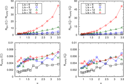
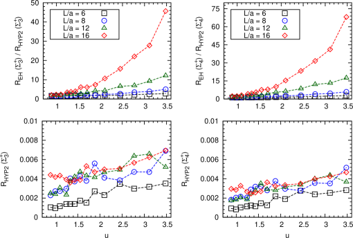
characteristic of the four chosen lattice discretizations of the static action. Here, $\Delta\Sigma_{k}^{\scriptscriptstyle+}$ denotes the statistical uncertainty of the SSF $\Sigma_{k}^{\scriptscriptstyle+}$, computed via the jackknife method. According to [20], $R_{\scriptscriptstyle\rm X}$ is related to the value of the binding energy $E_{\rm stat}\sim\frac{1}{a}e^{(1)}g_{0}^{2}~{}+~{}\dots$ of the static-light meson, which diverges linearly in the continuum limit. The leading coefficient $e^{(1)}$ depends upon the lattice discretization of the static action and its value sets the rate of growth of the noise-to-signal ratio: a linear reduction of $e^{(1)}$ corresponds indeed to an exponential damping of the statistical fluctuations. From our results we deduce the general trend

$$R_{\scriptscriptstyle\rm EH}\gg R_{\scriptscriptstyle\rm APE}\gtrsim R_{\scriptscriptstyle\rm HYP1}\gtrsim R_{\scriptscriptstyle\rm HYP2}\ .$$ (44)

As an example, we compare in Figures 2 and 2 the noise-to-signal ratio of the SSF of the operators $\{{{\cal Q}^{\prime}}_{k}^{\scriptscriptstyle+}\},k=1,\dots,4$ with EH and HYP2 discretizations in our preferred choice of the renormalization schemes. Lower plots in each figure show that $R_{\scriptscriptstyle\rm HYP2}$ is almost constant against variations in the renormalized coupling and always lower than $1\%$. Moreover, it never increases by more than a factor 4 going from the coarsest to the finest lattice resolution at fixed coupling. This picture is completely reversed when looking at the EH discretization, as shown in the upper plots. Here, a clear increase of the noise-to-signal ratio with the SF coupling and also with the lattice spacing is observed. In practice, the SSF has an acceptable uncertainty only in the perturbative region, i.e. for $u\lesssim\;1$. A comparison of the noise-to-signal ratio for different operators shows that in our preferred schemes $\Sigma^{\scriptscriptstyle+}_{1}$, $\Sigma^{\scriptscriptstyle+}_{2}$ and $\Sigma^{\scriptscriptstyle+}_{3}$ are slightly noisier than $\Sigma^{\scriptscriptstyle+}_{4}$ with the HYP2 action, in contrast to the EH one. Since the simulations with the EH action are practically unusable for our ultimate aims, the prevailing pattern is the one observed with the HYP2 discretization and will be reflected in the final statistical error of the RGI renormalization constants of the various operators.

5.2 Continuum extrapolation of the step scaling functions

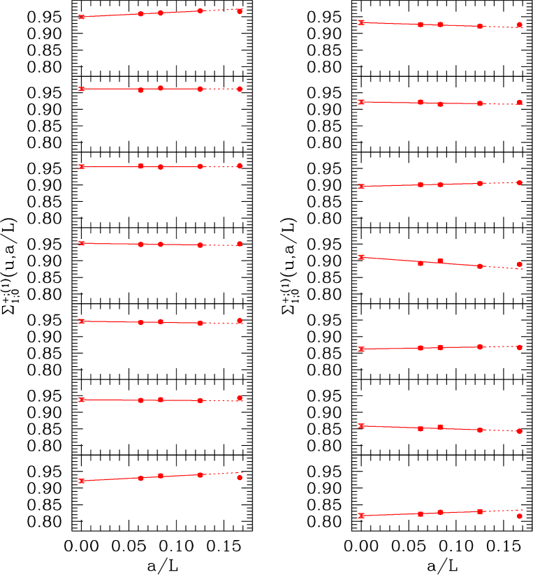
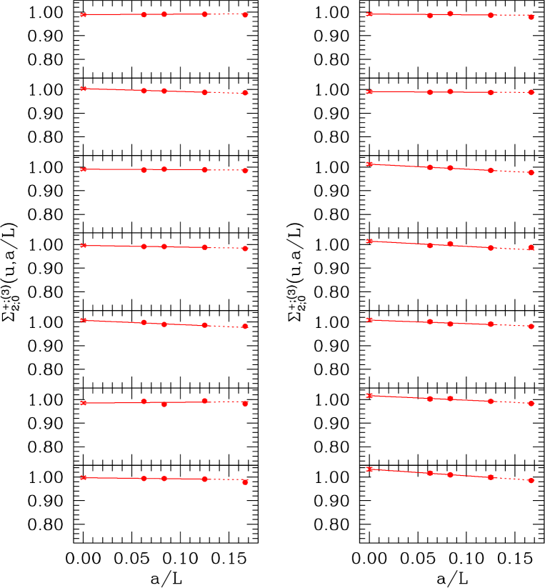
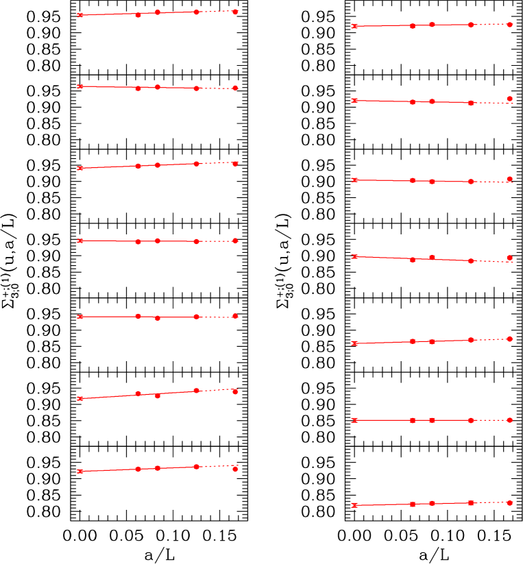
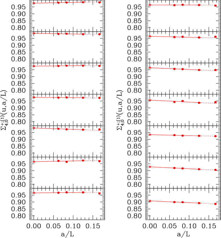
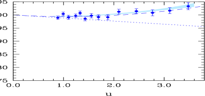
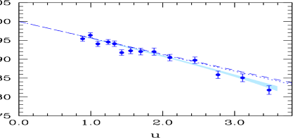
The lattice SSFs $\Sigma_{k}^{{\scriptscriptstyle+}}$ must be extrapolated to the continuum limit (i.e. to vanishing $a/L$) at fixed renormalized gauge coupling in order to obtain their continuum counterparts $\sigma_{k}^{{\scriptscriptstyle+}}$. Since the four-fermion operators have not been improved, we expect the dominant discretization effects to be $\mbox{O}(a)$; thus, our data should exhibit a linear behaviour in $a/L$. For every combination of $(s,\alpha)$ we have therefore fitted to the ansatz

$$\Sigma_{k}^{{\scriptscriptstyle+}}(u,a/L)=\sigma_{k}^{{\scriptscriptstyle+}}(u)+\rho(u)\,(a/L)\ .$$ (45)

Fits have been performed using either the whole available set of values of $L/a$ or, alternatively, without taking into account the data at $L/a=6$, which may be subject to higher-order lattice artefacts. Following the spirit of refs. [14, 11, 17], one could perform a combined fit of the data corresponding to the actions APE, HYP1 and HYP2, all of which have comparable noise-to-signal ratios in the range of lattice parameters covered in this work. However, data obtained with the above actions differ noticeably only – if ever – at $L/a=6$, and are very strongly correlated. As a consequence, a combined continuum extrapolation affects only marginally the result coming from the best choice of the action, i.e. HYP2, with a reduction of the relative error of $\sigma_{k}^{{\scriptscriptstyle+}}(u)$ at the level of a few percent. Thus, without any loss, we will consider only the HYP2 data from now on. Fit results can be summarized as follows:

1. the typical statistical accuracy of our results for $\sigma_{k}^{{\scriptscriptstyle+}}$ ranges from $\sim 0.5\%$ relative error, for the weakest couplings and fits that keep $L/a=6$, to $\sim 1.5\%$ relative error at the maximum value of $u$, for fits that discard $L/a=6$. When $L/a=6$ is dropped, the fitted values of $\rho$ are always essentially compatible with zero within the statistical uncertainty for ${{\cal Q}^{\prime}}^{\scriptscriptstyle+}_{1}$ and ${{\cal Q}^{\prime}}^{\scriptscriptstyle+}_{3}$, signalling a weak cutoff dependence of $\Sigma_{k}^{{\scriptscriptstyle+}}$. For ${{\cal Q}^{\prime}}^{\scriptscriptstyle+}_{2}$ and ${{\cal Q}^{\prime}}^{\scriptscriptstyle+}_{4}$, on the other hand, they are zero only within two standard deviations at $u\gtrsim 2$. In fits containing $L/a=6$, non-zero values of $\rho$ are usually obtained for the couplings $u\gtrsim 2$ and all the operators;

2. results from three-point and four-point fits are always compatible within one standard deviation for all operators and schemes, save for a few exceptions in which the agreement is at the level of $1.5\sigma$ only;

3. the goodness of fit, expressed by the value of $\chi^{2}$ per degree of freedom, is mostly around or below $1$, although it reaches large values in some cases. This does not depend systematically on the number of the fitted points or the value of the coupling. Anyway, given the small number of fitted data points, $\chi^{2}/\mbox{d.o.f.}$ for each single fit at fixed value of the coupling is a goodness-of-fit criterion of limited value; instead, the total $\chi^{2}/\mbox{d.o.f.}$ (summed over all values of the coupling at fixed operator and scheme) is always around or below $1$, reaching maxima of the order of $1.5$.

Based on this analysis, we conservatively choose linear extrapolations that do not consider the $L/a=6$ datum to extract our final values of $\sigma_{k}^{{\scriptscriptstyle+}}$. The resulting continuum limit extrapolations are illustrated in Figs. 3–6 for our reference schemes (chosen below). Complete tables with the results are available at [33].

5.3 RG running in the continuum limit

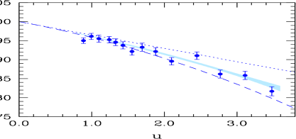
The analysis described above yields accurate estimates of the continuum SSFs $\sigma_{k}^{{\scriptscriptstyle+}}$ for a wide range of values of the renormalized coupling. In order to compute the RG running of the operators in the continuum limit as described in sect. 4, we need to fit these data, as well as those for the SSF of the renormalized coupling itself, to some functional form. Regarding the SSF of the coupling $\sigma(u)$, we have followed the same procedure as in [10]. This has been also adopted for the SSFs of the four-fermion operators, for which we have assumed the polynomial ansatz

$$\sigma_{k}^{{\scriptscriptstyle+}}=1+\sum_{n=1}^{N}s_{n}u^{n}\,,$$ (46)

motivated by the form of the perturbative series. In particular, the analytical expressions of the first two coefficients are given in perturbation theory by

$$s_{1}={\gamma^{\prime}}_{k}^{+;(0)}\ln 2\,,$$ (47)

$$s_{2}={\gamma^{\prime}}_{k}^{+;(1)}\ln 2+\left[\frac{1}{2}({\gamma^{\prime}}_{k}^{+;(0)})^{2}+b_{0}{\gamma^{\prime}}_{k}^{+;(0)}\right](\ln 2)^{2}\,.$$ (48)

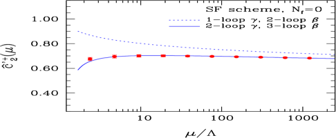
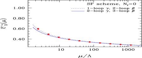
While the first coefficient is entirely determined by the LO anomalous dimension and is hence universal, the second one, where the NLO anomalous dimension enters, is scheme dependent. Contrary to the case of the fully relativistic four-quark operators considered in [34], the NLO coefficient does not depend strongly on the chosen SF scheme. We have performed fits to the ansatz of Eq. (46) with $N$ ranging from $2$ to $4$. The coefficient $s_{1}$ is always kept fixed to the value in Eq. (47), and fits are performed either with $s_{2}$ fixed to the value in Eq. (48) or keeping it as a free parameter. All fits are well behaved, with values of $\chi^{2}/\mbox{d.o.f.}$ ranging from $0.8$ to $1.6$. It is worth mentioning that when $s_{2}$ is kept as a free parameter, its fitted value lies in the ballpark of the perturbative prediction of Eq. (48), which can be taken as an indication that perturbation theory indeed describes the data well within a large part of the range of scales covered by our simulations. However, our data are not accurate enough to allow for a more detailed check of the applicability of perturbation theory beyond leading order. Once a definite expression for the fitted step scaling function is chosen, the solution of the recursion relations provided by Eqs. (33) and (25) is unique. At that point, the value obtained for the RG running factor ${U^{\prime}}_{k}^{{\scriptscriptstyle+}}(2^{n}\mu_{\rm had},\mu_{\rm had})$ of Eq. (25) is a function of the fit parameters only. We have checked that increasing the number of fit parameters provides compatible results for ${U^{\prime}}_{k}^{{\scriptscriptstyle+}}(2^{n}\mu_{\rm had},\mu_{\rm had})$ with slightly larger errors. The result is also fairly insensitive to whether $s_{2}$ is fixed to the perturbative prediction or not. The conclusion is that, at the available level of precision, the bias induced by the choice of the fit function is not significant, which results in a numerically very stable determination of the SSFs. We quote as our best results those coming from a two-parameter fit with $s_{1}$ fixed by perturbation theory. At this point it is useful to restrict the attention to a selected subset of renormalization schemes. As discussed in [3], heavy quark spin symmetry provides a number of identities between the 10 SF schemes we have considered per operator. In practice, we have four different independent schemes for the operators ${{\cal Q}^{\prime}}^{\scriptscriptstyle+}_{1}$ and ${{\cal Q}^{\prime}}^{\scriptscriptstyle+}_{3}$, and another eight for ${{\cal Q}^{\prime}}^{\scriptscriptstyle+}_{2}$ and ${{\cal Q}^{\prime}}^{\scriptscriptstyle+}_{4}$. All these schemes should lead to the same RGI quantities, since the total renormalization factors (see below) differ only by cutoff effects. This could be used potentially to improve continuum limit extrapolations by combining various schemes. However, the strong statistical correlation between the different renormalization factors is likely to produce only a small gain in precision. Therefore, we choose for each operator just one single representative scheme. This strategy has been seen to be justified in the fully relativistic case, i.e. in the computation of $B_{K}$ [18, 19]. As discussed in [17], the main criterion to define suitable schemes amounts to checking that the systematic uncertainty related to truncating at NLO the perturbative matching at the scale $\mu_{\rm pt}\equiv 2^{n}\mu_{\rm had}$ in Eq. (23) is well under control. This in turn requires an estimate of the size of the NNLO contribution to ${\hat{c}}^{\prime{\scriptscriptstyle+}}_{\>k}(\mu_{\rm pt})$. To this purpose we have re-computed ${\hat{c}}^{\prime{\scriptscriptstyle+}}_{\>k}(\mu_{\rm pt})$ with two different values of the NNLO anomalous dimensions ${\gamma^{\prime}}^{+;(2)}_{k}$: in the first case we set ${\gamma^{\prime}}^{+;(2)}_{k}/{\gamma^{\prime}}^{+;(1)}_{k}={\gamma^{\prime}}^{+;(1)}_{k}/{\gamma^{\prime}}^{+;(0)}_{k}$; in the second case, we guess ${\gamma^{\prime}}^{+;(2)}_{k}$ by performing a one-parameter fit to the SSF with $s_{1}$ and $s_{2}$ fixed by perturbation theory, and then equating the resulting value of $s_{3}$ to its perturbative expression

$$\begin{split}s_{3}={\gamma^{\prime}}^{+;(2)}_{k}\ln 2&+\left[{\gamma^{\prime}}^{+;(0)}_{k}{\gamma^{\prime}}^{+;(1)}_{k}+2b_{0}{\gamma^{\prime}}^{+;(1)}_{k}+b_{1}{\gamma^{\prime}}^{+;(0)}_{k}\right](\ln 2)^{2}+\\[8.61108pt] &+\left[\frac{1}{6}\left({\gamma^{\prime}}^{+;(0)}_{k}\right)^{3}+b_{0}\left({\gamma^{\prime}}^{+;(0)}_{k}\right)^{2}+\frac{4}{3}b_{0}^{2}{\gamma^{\prime}}^{+;(0)}_{k}\right](\ln 2)^{3}\,.\end{split}$$ (49)

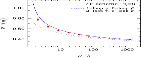
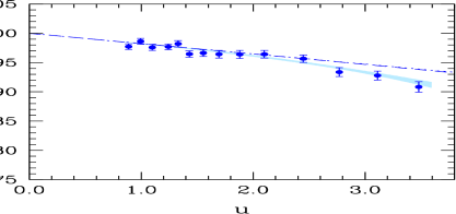
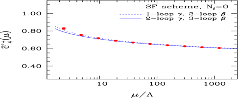
For the operators ${{\cal Q}^{\prime}}^{\scriptscriptstyle+}_{1,3,4}$, we find that in either case the central value of the combination ${\hat{c}}^{\prime{\scriptscriptstyle+}}_{\>k}(\mu_{\rm had})\equiv{\hat{c}}^{\prime{\scriptscriptstyle+}}_{\>k}(\mu_{\rm pt}){U^{\prime}}^{\scriptscriptstyle+}_{k}(\mu_{\rm pt},\mu_{\rm had})$ changes by a small fraction of the statistical error, of the order $0.1\sigma$–$0.3\sigma$. There is no systematic dependence on the choice of boundary operators or normalization factors in the renormalization condition. We thus conclude that this particular uncertainty is well covered by the statistical one and choose as our reference schemes those labeled by $(s,\alpha)=(1,0)$. As for the operator ${{\cal Q}^{\prime}}^{\scriptscriptstyle+}_{2}$, which carries relatively large NLO anomalous dimensions, the effect can be as large as $0.8\sigma$ with $s=3$, and of the order of $1\sigma$ with the other values of $s$. There is no significant dependence on $\alpha$. We therefore opt, conservatively, for $(s,\alpha)=(3,0)$ as our preferred choice for this operator, adding to ${\hat{c}}^{\prime{\scriptscriptstyle+}}_{\>2}(\mu_{\rm had})$ a systematic uncertainty of $0.8$ standard deviations. It has to be stressed that the impact of this extra uncertainty at the level of the $B$–$\bar{B}$ mixing amplitude is not particularly worrying, since the matrix element of ${{\cal Q}^{\prime}}^{\scriptscriptstyle+}_{2}$ enters the latter only at ${\cal O}(\alpha_{\rm s})$ when the static theory is matched to QCD. It is therefore expected to contribute a relatively small fraction to the final uncertainty. The results for the operator RG running in these schemes are provided in Table 1. Those concerning the SSFs are collected in Table 10. The same results are illustrated by Figure 7.

5.4 Matching to hadronic observables

The RGI operator, defined in Eq. (20), is connected to its bare counterpart via a total renormalization factor $\hat{Z}^{\prime{\scriptscriptstyle+}}_{\ k,{\rm\scriptscriptstyle RGI}}(g_{0})$, as in Eq. (28). We stress that $\hat{Z}^{\prime{\scriptscriptstyle+}}_{\ k,{\rm\scriptscriptstyle RGI}}(g_{0})$ is a scale-independent quantity, which moreover depends on the renormalization scheme only via cutoff effects. Indeed, it depends on the particular lattice regularization chosen, though only through the factor ${{\cal Z}^{\prime}}_{k}^{{\scriptscriptstyle+}}(g_{0},a\mu_{\rm had})$, the computation of which is much less expensive than the total RG running factor ${\hat{c}}^{\prime{\scriptscriptstyle+}}_{\>k}(\mu_{\rm had})$. We have computed ${{\cal Z}^{\prime}}_{k}^{+}(g_{0},a\mu_{\rm had}),\mu_{\rm{had}}=1/(2L_{\rm max})$ non-perturbatively at four values of $\beta$ for each scheme and four-fermion operator, and for the four different static actions under consideration. The results for the HYP2 action and the reference renormalization schemes defined in sect. 5.3 are given in Table 11. Upon multiplying by the corresponding running factors in Table 1, the total renormalization factors are obtained. These can be further fitted to polynomials of the form

$$\hat{Z}^{\prime{\scriptscriptstyle+}}_{\ k,{\rm\scriptscriptstyle RGI}}(g_{0})=a_{k}+b_{k}(\beta-6)+c_{k}(\beta-6)^{2}\,,$$ (50)

which can be subsequently used to obtain the total renormalization factor at any value of $\beta$ within the covered range. We provide in Table 1 the resulting fit coefficients for the HYP2 action in our reference renormalization schemes. These parameterizations represent our data with an accuracy of at least $0.3\%$ (this comprises the point $\beta=6.0$. The contribution from the error in the RG running factors of Table 1 has been neglected: since these factors have been computed in the continuum limit, they should be added in quadrature after the quantity renormalized with the factor derived from Eq. (50) has been extrapolated itself to the continuum limit.

$k$	$s$	${\hat{c}}^{\prime{\scriptscriptstyle+};(s)}_{\>k;0}(\mu_{\rm had})$	$~{}~{}~{}~{}a_{k;0}^{(s)}$	$~{}~{}~{}~{}b_{k;0}^{(s)}$	$~{}~{}~{}c_{k;0}^{(s)}$
$1$	$1$	$0.777(17)$	$0.5731(11)$	$-0.171(11)$	$0.082(25)$
$2^{*}$	$3$	$0.675(12)$	$0.7258(14)$	$-0.061(14)$	$0.016(33)$
$3$	$1$	$0.598(12)$	$0.4564(8)$	$-0.142(8)$	$0.068(18)$
$4$	$1$	$0.828(11)$	$0.6465(9)$	$-0.070(9)$	$0.033(21)$

Table 1: Running factor ${\hat{c}}^{\prime{\scriptscriptstyle+};(s)}_{\>k;0}(\mu_{\rm had})$ and fit coefficients (see Eq. (50)) to the total renormalization factor $\hat{Z}^{\prime{\scriptscriptstyle+}}_{\ k,{\rm\scriptscriptstyle RGI}}(g_{0})$ introduced in Eq. (28). Here $\mu_{\rm had}^{-1}=2L_{\rm max}$. The schemes characterized by larger systematic uncertainties related to perturbation theory have been indicated with an asterisk.

6 Conclusions

$B^{0}-\bar{B}^{0}$ mixing remains among the most important processes that are required to pin down the elements of the CKM matrix precisely. However, in order to constrain the unitarity triangle sufficiently well and to look for signs of new physics, theoretical uncertainties associated with hadronic effects must be further reduced. Non-perturbative renormalization of four-quark operators is an indispensable ingredient to enable lattice determinations of the corresponding hadronic matrix elements with a total accuracy at the level of a few percent. In this paper we have described our fully non-perturbative calculation of the relations between parity-odd, static-light four-quark operators in quenched lattice QCD and their renormalized counterparts. Our main results for the complete basis of operators are expressed by the interpolating formula of Eq. (50), in conjunction with the coefficients listed in Table 1. In addition to the regularization-dependent, total renormalization factors $\hat{Z^{\prime}}^{\scriptscriptstyle+}_{k,{\rm\scriptscriptstyle RGI}}$, we also list the universal running factors ${\hat{c}}^{\prime{\scriptscriptstyle+}}_{\>k}(\mu_{\rm had})$, which, if desired, can be combined with a different fermionic discretization, provided that the regularization-dependent matching factor ${{\cal Z}^{\prime}}_{k}^{\scriptscriptstyle+}(g_{0},a\mu_{\rm had})$ (c.f. Eq. (28)) is re-computed. The bulk of the uncertainty associated with the renormalization originates from the universal running factors, which have been determined with an accuracy of $1.5-2$%. The level of precision ensures that the targeted accuracy of, say, 5% in the final result for the $B$-parameters in the continuum limit can be reached. The calculation of the bare hadronic matrix elements in quenched twisted mass QCD is currently underway. Finally, we stress that our method can be straightforwardly extended to the unquenched case, with the simulations to compute the step scaling functions for $N_{\rm\scriptsize f}=2$ dynamical quark flavours currently in progress [35]. Although Ginsparg-Wilson fermions appear as the natural discretization to study left-left four-quark operators, the Schrödinger functional is far more complicated to implement than for Wilson-like fermions. In our approach, tmQCD serves to solve the intricate renormalization problem for four-quark operators, while the SF scheme is easy to implement and dynamical simulations with Wilson fermions can be performed in an economical way.

Appendix A Tables and figures

$~{}~{}~{}~{}~{}~{}~{}\beta~{}~{}~{}~{}$	${L}/{a}$	$~{}~{}~{}\bar{g}^{2}_{\rm\scriptscriptstyle SF}(L)$	$~{}~{}~{}~{}~{}\kappa_{\rm cr}$	$\mathcal{Z^{\prime}}_{1;0}^{+;(1)}\left(g_{0},{a}/{L}\right)$	$\mathcal{Z^{\prime}}_{1;0}^{+;(1)}\left(g_{0},{a}/{2L}\right)$	${\Sigma}^{+;(1)}_{1;0}\left(g_{0},{a}/{L}\right)$
10.7503	6	0.8873(5)	0.130591(4)	0.9136(8)	0.8827(12)	0.9662(15)
11.0000	8	0.8873(10)	0.130439(3)	0.9041(7)	0.8751(24)	0.9679(28)
11.3384	12	0.8873(30)	0.130251(2)	0.8912(7)	0.8571(26)	0.9617(30)
11.5736	16	0.8873(25)	0.130125(2)	0.8827(14)	0.8467(35)	0.9592(43)
10.0500	6	0.9944(7)	0.131073(5)	0.9073(8)	0.8714(8)	0.9604(12)
10.3000	8	0.9944(13)	0.130889(3)	0.8943(8)	0.8590(28)	0.9605(32)
10.6086	12	0.9944(30)	0.130692(2)	0.8798(7)	0.8478(25)	0.9636(30)
10.8910	16	0.9944(28)	0.130515(2)	0.8737(25)	0.8365(34)	0.9574(47)
9.5030	6	1.0989(8)	0.131514(5)	0.8992(9)	0.8611(11)	0.9576(15)
9.7500	8	1.0989(13)	0.131312(3)	0.8876(8)	0.8484(33)	0.9558(38)
10.0577	12	1.0989(40)	0.131079(3)	0.8713(10)	0.8311(32)	0.9539(38)
10.3419	16	1.0989(44)	0.130876(2)	0.8645(33)	0.8274(33)	0.9571(53)
8.8997	6	1.2430(13)	0.132072(9)	0.8894(9)	0.8459(12)	0.9511(17)
9.1544	8	1.2430(14)	0.131838(4)	0.8781(9)	0.8314(34)	0.9468(40)
9.5202	12	1.2430(35)	0.131503(3)	0.8613(8)	0.8177(23)	0.9494(28)
9.7350	16	1.2430(34)	0.131335(3)	0.8490(19)	0.8058(31)	0.9491(42)
8.6129	6	1.3293(12)	0.132380(6)	0.8854(10)	0.8391(12)	0.9477(17)
8.8500	8	1.3293(21)	0.132140(5)	0.8714(9)	0.8192(41)	0.9401(48)
9.1859	12	1.3293(60)	0.131814(3)	0.8545(12)	0.8069(35)	0.9443(43)
9.4381	16	1.3293(40)	0.131589(2)	0.8400(18)	0.7915(30)	0.9423(41)
8.3124	6	1.4300(20)	0.132734(10)	0.8810(10)	0.8308(12)	0.9430(17)
8.5598	8	1.4300(21)	0.132453(5)	0.8668(10)	0.8104(39)	0.9349(46)
8.9003	12	1.4300(50)	0.132095(3)	0.8474(9)	0.7947(40)	0.9378(48)
9.1415	16	1.4300(58)	0.131855(3)	0.8304(18)	0.7770(31)	0.9357(43)
7.9993	6	1.5553(15)	0.133118(7)	0.8725(10)	0.8126(14)	0.9313(20)
8.2500	8	1.5553(24)	0.132821(5)	0.8573(11)	0.8051(40)	0.9391(48)
8.5985	12	1.5533(70)	0.132427(3)	0.8380(20)	0.7850(39)	0.9368(52)
8.8323	16	1.5533(70)	0.132169(3)	0.8261(19)	0.7677(32)	0.9293(44)

Table 2: Numerical values of the renormalization constant $\mathcal{Z^{\prime}}_{1;0}^{+;(1)}$ and the step scaling function ${\Sigma}_{1;0}^{+;(1)}$ with HYP2 action at various renormalized SF couplings and lattice spacings.

$~{}~{}~{}~{}~{}~{}~{}\beta~{}~{}~{}~{}$	${L}/{a}$	$~{}~{}~{}\bar{g}^{2}_{\rm\scriptscriptstyle SF}(L)$	$~{}~{}~{}~{}~{}\kappa_{\rm cr}$	$\mathcal{Z^{\prime}}_{1;0}^{+;(1)}\left(g_{0},{a}/{L}\right)$	$\mathcal{Z^{\prime}}_{1;0}^{+;(1)}\left(g_{0},{a}/{2L}\right)$	${\Sigma}_{1;0}^{+;(1)}\left(g_{0},{a}/{L}\right)$
7.7170	6	1.6950(26)	0.133517(8)	0.8664(11)	0.8024(10)	0.9261(17)
7.9741	8	1.6950(28)	0.133179(5)	0.8503(9)	0.7836(40)	0.9216(48)
8.3218	12	1.6950(79)	0.132756(4)	0.8292(10)	0.7684(37)	0.9267(46)
8.5479	16	1.6950(90)	0.132485(3)	0.8154(21)	0.7553(41)	0.9263(55)
7.4082	6	1.8811(22)	0.133961(8)	0.8571(12)	0.7891(24)	0.9207(30)
7.6547	8	1.8811(28)	0.133632(6)	0.8399(11)	0.7705(38)	0.9174(47)
7.9993	12	1.8811(38)	0.133159(4)	0.8192(15)	0.7493(35)	0.9147(46)
8.2415	16	1.8811(99)	0.132847(3)	0.7983(28)	0.7356(30)	0.9215(50)
7.1214	6	2.1000(39)	0.134423(9)	0.8478(13)	0.7687(17)	0.9067(24)
7.3632	8	2.1000(45)	0.134088(6)	0.8304(12)	0.7512(33)	0.9046(42)
7.6985	12	2.1000(80)	0.133599(4)	0.8040(15)	0.7241(34)	0.9006(46)
7.9560	16	2.100(11)	0.133229(3)	0.7889(21)	0.7107(36)	0.9009(51)
6.7807	6	2.4484(37)	0.134994(11)	0.8339(21)	0.7414(22)	0.8891(35)
7.0197	8	2.4484(45)	0.134639(7)	0.8124(13)	0.7173(28)	0.8829(38)
7.3551	12	2.4484(80)	0.134141(5)	0.7867(19)	0.7079(34)	0.8998(48)
7.6101	16	2.448(17)	0.133729(4)	0.7734(25)	0.6899(34)	0.8920(53)
6.5512	6	2.770(7)	0.135327(12)	0.8245(15)	0.7146(20)	0.8667(29)
6.7860	8	2.770(7)	0.135056(8)	0.7995(14)	0.6946(36)	0.8688(48)
7.1190	12	2.770(11)	0.134513(5)	0.7731(14)	0.6700(40)	0.8666(54)
7.3686	16	2.770(14)	0.134114(3)	0.7546(24)	0.6531(34)	0.8655(53)
6.3665	6	3.111(4)	0.135488(6)	0.8166(15)	0.6884(20)	0.8430(29)
6.6100	8	3.111(6)	0.135339(3)	0.7902(14)	0.6688(32)	0.8464(43)
6.9322	12	3.111(12)	0.134855(3)	0.7585(18)	0.6487(42)	0.8552(59)
7.1911	16	3.111(16)	0.134411(3)	0.7399(24)	0.6291(36)	0.8503(56)
6.2204	6	3.480(8)	0.135470(15)	0.8062(16)	0.6574(21)	0.8154(30)
6.4527	8	3.480(14)	0.135543(9)	0.7791(14)	0.6458(44)	0.8289(59)
6.7750	12	3.480(39)	0.135121(5)	0.7452(18)	0.6162(30)	0.8269(46)
7.0203	16	3.480(21)	0.134707(4)	0.7243(22)	0.5951(39)	0.8216(60)

Table 3: Numerical values of the renormalization constant $\mathcal{Z^{\prime}}_{1;0}^{+;(1)}$ and the step scaling function ${\Sigma}_{1;0}^{+;(1)}$ with HYP2 action at various renormalized SF couplings and lattice spacings (continued).

$~{}~{}~{}~{}~{}~{}~{}\beta~{}~{}~{}~{}$	${L}/{a}$	$~{}~{}~{}\bar{g}^{2}_{\rm\scriptscriptstyle SF}(L)$	$~{}~{}~{}~{}~{}\kappa_{\rm cr}$	$\mathcal{Z^{\prime}}_{2;0}^{+;(3)}\left(g_{0},{a}/{L}\right)$	$\mathcal{Z^{\prime}}_{2;0}^{+;(3)}\left(g_{0},{a}/{2L}\right)$	${\Sigma}_{2;0}^{+;(3)}\left(g_{0},{a}/{L}\right)$
10.7503	6	0.8873(5)	0.130591(4)	1.0020(7)	0.9905(11)	0.9885(13)
11.0000	8	0.8873(10)	0.130439(3)	0.9936(7)	0.9847(24)	0.9910(25)
11.3384	12	0.8873(30)	0.130251(2)	0.9885(6)	0.9798(24)	0.9912(25)
11.5736	16	0.8873(25)	0.130125(2)	0.9851(13)	0.9744(36)	0.9891(39)
10.0500	6	0.9944(7)	0.131073(5)	1.0033(8)	0.9897(8)	0.9864(11)
10.3000	8	0.9944(13)	0.130889(3)	0.9956(7)	0.9838(26)	0.9881(27)
10.6086	12	0.9944(30)	0.130692(2)	0.9881(6)	0.9825(24)	0.9943(25)
10.8910	16	0.9944(28)	0.130515(2)	0.9835(23)	0.9786(31)	0.9950(39)
9.5030	6	1.0989(8)	0.131514(5)	1.0040(9)	0.9886(10)	0.9847(13)
9.7500	8	1.0989(13)	0.131312(3)	0.9966(8)	0.9851(30)	0.9885(31)
10.0577	12	1.0989(40)	0.131079(3)	0.9891(10)	0.9806(27)	0.9914(29)
10.3419	16	1.0989(44)	0.130876(2)	0.9876(30)	0.9752(34)	0.9874(45)
8.8997	6	1.2430(13)	0.132072(9)	1.0061(10)	0.9888(12)	0.9828(15)
9.1544	8	1.2430(14)	0.131838(4)	0.9978(9)	0.9858(31)	0.9880(33)
9.5202	12	1.2430(35)	0.131503(3)	0.9889(8)	0.9807(23)	0.9917(24)
9.7350	16	1.2430(34)	0.131335(3)	0.9835(18)	0.9751(32)	0.9915(37)
8.6129	6	1.3293(12)	0.132380(6)	1.0095(11)	0.9918(13)	0.9825(16)
8.8500	8	1.3293(21)	0.132140(5)	0.9994(10)	0.9860(39)	0.9866(40)
9.1859	12	1.3293(60)	0.131814(3)	0.9898(12)	0.9794(30)	0.9895(33)
9.4381	16	1.3293(40)	0.131589(2)	0.9828(17)	0.9813(30)	0.9985(35)
8.3124	6	1.4300(20)	0.132734(10)	1.0101(11)	0.9921(12)	0.9822(16)
8.5598	8	1.4300(21)	0.132453(5)	0.9986(10)	0.9927(45)	0.9941(46)
8.9003	12	1.4300(50)	0.132095(3)	0.9926(9)	0.9724(36)	0.9796(37)
9.1415	16	1.4300(58)	0.131855(3)	0.9864(20)	0.9790(28)	0.9925(35)
7.9993	6	1.5553(15)	0.133118(7)	1.0139(12)	0.9909(16)	0.9773(20)
8.2500	8	1.5553(24)	0.132821(5)	1.0015(12)	0.9926(41)	0.9911(43)
8.5985	12	1.5533(70)	0.132427(3)	0.9915(20)	0.9855(43)	0.9939(47)
8.8323	16	1.5533(70)	0.132169(3)	0.9844(19)	0.9784(33)	0.9939(38)

Table 4: Numerical values of the renormalization constant $\mathcal{Z^{\prime}}_{2;0}^{+;(3)}$ and the step scaling function ${\Sigma}_{2;0}^{+;(3)}$ with HYP2 action at various renormalized SF couplings and lattice spacings.

$~{}~{}~{}~{}~{}~{}~{}\beta~{}~{}~{}~{}$	${L}/{a}$	$~{}~{}~{}\bar{g}^{2}_{\rm\scriptscriptstyle SF}(L)$	$~{}~{}~{}~{}~{}\kappa_{\rm cr}$	$\mathcal{Z^{\prime}}_{2;0}^{+;(3)}\left(g_{0},{a}/{L}\right)$	$\mathcal{Z^{\prime}}_{2;0}^{+;(3)}\left(g_{0},{a}/{2L}\right)$	${\Sigma}_{2;0}^{+;(3)}\left(g_{0},{a}/{L}\right)$
7.7170	6	1.6950(26)	0.133517(8)	1.0153(13)	0.9938(12)	0.9788(17)
7.9741	8	1.6950(28)	0.133179(5)	1.0025(10)	0.9892(40)	0.9867(41)
8.3218	12	1.6950(79)	0.132756(4)	0.9928(11)	0.9866(37)	0.9938(39)
8.5479	16	1.6950(90)	0.132485(3)	0.9897(21)	0.9753(43)	0.9855(49)
7.4082	6	1.8811(22)	0.133961(8)	1.0137(13)	1.0021(26)	0.9886(28)
7.6547	8	1.8811(28)	0.133632(6)	1.0051(13)	0.9927(56)	0.9877(57)
7.9993	12	1.8811(38)	0.133159(4)	0.9917(16)	0.9835(34)	0.9917(38)
8.2415	16	1.8811(99)	0.132847(3)	0.9876(30)	0.9762(31)	0.9885(44)
7.1214	6	2.1000(39)	0.134423(9)	1.0249(15)	1.0011(21)	0.9768(25)
7.3632	8	2.1000(45)	0.134088(6)	1.0113(14)	0.9971(43)	0.9860(45)
7.6985	12	2.1000(80)	0.133599(4)	0.9944(17)	0.9911(43)	0.9967(46)
7.9560	16	2.100(11)	0.133229(3)	0.9857(22)	0.9841(39)	0.9984(46)
6.7807	6	2.4484(37)	0.134994(11)	1.0276(25)	1.0153(30)	0.9880(38)
7.0197	8	2.4484(45)	0.134639(7)	1.0158(15)	1.0013(35)	0.9857(37)
7.3551	12	2.4484(80)	0.134141(5)	1.0005(21)	1.0035(43)	1.0030(48)
7.6101	16	2.448(17)	0.133729(4)	0.9965(30)	0.9923(39)	0.9958(49)
6.5512	6	2.770(7)	0.135327(12)	1.0371(19)	1.0174(27)	0.9810(31)
6.7860	8	2.770(7)	0.135056(8)	1.0233(17)	1.0144(55)	0.9913(56)
7.1190	12	2.770(11)	0.134513(5)	1.0054(17)	0.9972(54)	0.9918(56)
7.3686	16	2.770(14)	0.134114(3)	0.9959(30)	0.9976(45)	1.0017(54)
6.3665	6	3.111(4)	0.135488(6)	1.0494(21)	1.0317(31)	0.9831(35)
6.6100	8	3.111(6)	0.135339(3)	1.0269(18)	1.0191(44)	0.9924(46)
6.9322	12	3.111(12)	0.134855(3)	1.0156(24)	1.0200(55)	1.0043(59)
7.1911	16	3.111(16)	0.134411(3)	0.9981(30)	1.0006(49)	1.0025(57)
6.2204	6	3.480(8)	0.135470(15)	1.0544(22)	1.0390(33)	0.9854(37)
6.4527	8	3.480(14)	0.135543(9)	1.0345(20)	1.0330(68)	0.9986(69)
6.7750	12	3.480(39)	0.135121(5)	1.0186(24)	1.0279(46)	1.0091(51)
7.0203	16	3.480(21)	0.134707(4)	1.0067(29)	1.0233(58)	1.0165(65)

Table 5: Numerical values of the renormalization constant $\mathcal{Z^{\prime}}_{2;0}^{+;(3)}$ and the step scaling function ${\Sigma}_{2;0}^{+;(3)}$ with HYP2 action at various renormalized SF couplings and lattice spacings (continued).

$~{}~{}~{}~{}~{}~{}~{}\beta~{}~{}~{}~{}$	${L}/{a}$	$~{}~{}~{}\bar{g}^{2}_{\rm\scriptscriptstyle SF}(L)$	$~{}~{}~{}~{}~{}\kappa_{\rm cr}$	$\mathcal{Z^{\prime}}_{3;0}^{+;(1)}\left(g_{0},{a}/{L}\right)$	$\mathcal{Z^{\prime}}_{3;0}^{+;(1)}\left(g_{0},{a}/{2L}\right)$	${\Sigma}_{3;0}^{+;(1)}\left(g_{0},{a}/{L}\right)$
10.7503	6	0.8873(5)	0.130591(4)	0.9377(5)	0.9039(8)	0.9640(10)
11.0000	8	0.8873(10)	0.130439(3)	0.9250(5)	0.8913(20)	0.9636(22)
11.3384	12	0.8873(30)	0.130251(2)	0.9093(5)	0.8758(21)	0.9632(24)
11.5736	16	0.8873(25)	0.130125(2)	0.8987(12)	0.8578(36)	0.9545(42)
10.0500	6	0.9944(7)	0.131073(5)	0.9313(6)	0.8926(6)	0.9584(9)
10.3000	8	0.9944(13)	0.130889(3)	0.9180(6)	0.8785(23)	0.9570(26)
10.6086	12	0.9944(30)	0.130692(2)	0.8993(5)	0.8647(20)	0.9615(23)
10.8910	16	0.9944(28)	0.130515(2)	0.8886(19)	0.8504(30)	0.9570(40)
9.5030	6	1.0989(8)	0.131514(5)	0.9258(7)	0.8830(8)	0.9538(11)
9.7500	8	1.0989(13)	0.131312(3)	0.9114(6)	0.8693(23)	0.9538(26)
10.0577	12	1.0989(40)	0.131079(3)	0.8921(8)	0.8473(25)	0.9498(29)
10.3419	16	1.0989(44)	0.130876(2)	0.8833(24)	0.8364(28)	0.9469(41)
8.8997	6	1.2430(13)	0.132072(9)	0.9182(7)	0.8687(10)	0.9461(13)
9.1544	8	1.2430(14)	0.131838(4)	0.9034(7)	0.8523(25)	0.9434(28)
9.5202	12	1.2430(35)	0.131503(3)	0.8825(7)	0.8346(18)	0.9457(22)
9.7350	16	1.2430(34)	0.131335(3)	0.8677(14)	0.8180(29)	0.9427(37)
8.6129	6	1.3293(12)	0.132380(6)	0.9145(8)	0.8626(10)	0.9432(13)
8.8500	8	1.3293(21)	0.132140(5)	0.8968(7)	0.8435(33)	0.9406(38)
9.1859	12	1.3293(60)	0.131814(3)	0.8763(9)	0.8206(29)	0.9364(35)
9.4381	16	1.3293(40)	0.131589(2)	0.8588(14)	0.8093(26)	0.9424(34)
8.3124	6	1.4300(20)	0.132734(10)	0.9093(8)	0.8534(10)	0.9385(13)
8.5598	8	1.4300(21)	0.132453(5)	0.8918(8)	0.8405(31)	0.9425(35)
8.9003	12	1.4300(50)	0.132095(3)	0.8702(7)	0.8058(33)	0.9260(39)
9.1415	16	1.4300(58)	0.131855(3)	0.8535(16)	0.7962(26)	0.9329(36)
7.9993	6	1.5553(15)	0.133118(7)	0.9035(9)	0.8395(12)	0.9292(16)
8.2500	8	1.5553(24)	0.132821(5)	0.8846(9)	0.8284(34)	0.9365(40)
8.5985	12	1.5533(70)	0.132427(3)	0.8600(16)	0.8018(35)	0.9323(44)
8.8323	16	1.5533(70)	0.132169(3)	0.8426(15)	0.7830(27)	0.9293(36)

Table 6: Numerical values of the renormalization constant $\mathcal{Z^{\prime}}_{3;0}^{+;(1)}$ and the step scaling function ${\Sigma}_{3;0}^{+;(1)}$ with HYP2 action at various renormalized SF couplings and lattice spacings.

$~{}~{}~{}~{}~{}~{}~{}\beta~{}~{}~{}~{}$	${L}/{a}$	$~{}~{}~{}\bar{g}^{2}_{\rm\scriptscriptstyle SF}(L)$	$~{}~{}~{}~{}~{}\kappa_{\rm cr}$	$\mathcal{Z^{\prime}}_{3;0}^{+;(1)}\left(g_{0},{a}/{L}\right)$	$\mathcal{Z^{\prime}}_{3;0}^{+;(1)}\left(g_{0},{a}/{2L}\right)$	${\Sigma}_{3;0}^{+;(1)}\left(g_{0},{a}/{L}\right)$
7.7170	6	1.6950(26)	0.133517(8)	0.8969(9)	0.8296(9)	0.9250(14)
7.9741	8	1.6950(28)	0.133179(5)	0.8773(7)	0.8111(30)	0.9245(35)
8.3218	12	1.6950(79)	0.132756(4)	0.8515(8)	0.7881(33)	0.9255(40)
8.5479	16	1.6950(90)	0.132485(3)	0.8356(16)	0.7693(38)	0.9207(49)
7.4082	6	1.8811(22)	0.133961(8)	0.8868(10)	0.8210(20)	0.9258(25)
7.6547	8	1.8811(28)	0.133632(6)	0.8674(9)	0.7913(44)	0.9123(51)
7.9993	12	1.8811(38)	0.133159(4)	0.8400(13)	0.7706(30)	0.9174(38)
8.2415	16	1.8811(99)	0.132847(3)	0.8192(25)	0.7497(27)	0.9152(43)
7.1214	6	2.1000(39)	0.134423(9)	0.8809(11)	0.7993(15)	0.9074(21)
7.3632	8	2.1000(45)	0.134088(6)	0.8594(10)	0.7731(30)	0.8996(37)
7.6985	12	2.1000(80)	0.133599(4)	0.8261(13)	0.7430(32)	0.8994(42)
7.9560	16	2.100(11)	0.133229(3)	0.8077(18)	0.7293(32)	0.9029(45)
6.7807	6	2.4484(37)	0.134994(11)	0.8664(18)	0.7746(21)	0.8940(31)
7.0197	8	2.4484(45)	0.134639(7)	0.8434(10)	0.7454(27)	0.8838(34)
7.3551	12	2.4484(80)	0.134141(5)	0.8097(16)	0.7245(32)	0.8948(44)
7.6101	16	2.448(17)	0.133729(4)	0.7931(22)	0.7036(30)	0.8872(45)
6.5512	6	2.770(7)	0.135327(12)	0.8572(13)	0.7481(19)	0.8727(26)
6.7860	8	2.770(7)	0.135056(8)	0.8303(11)	0.7221(33)	0.8697(41)
7.1190	12	2.770(11)	0.134513(5)	0.7979(12)	0.6895(42)	0.8641(55)
7.3686	16	2.770(14)	0.134114(3)	0.7753(22)	0.6707(33)	0.8651(49)
6.3665	6	3.111(4)	0.135488(6)	0.8488(13)	0.7229(20)	0.8517(27)
6.6100	8	3.111(6)	0.135339(3)	0.8182(12)	0.6960(31)	0.8506(40)
6.9322	12	3.111(12)	0.134855(3)	0.7832(17)	0.6666(41)	0.8511(56)
7.1911	16	3.111(16)	0.134411(3)	0.7593(22)	0.6458(36)	0.8505(53)
6.2204	6	3.480(8)	0.135470(15)	0.8384(14)	0.6920(22)	0.8254(29)
6.4527	8	3.480(14)	0.135543(9)	0.8074(13)	0.6668(45)	0.8259(57)
6.7750	12	3.480(39)	0.135121(5)	0.7715(16)	0.6361(30)	0.8245(43)
7.0203	16	3.480(21)	0.134707(4)	0.7445(21)	0.6115(39)	0.8214(57)

Table 7: Numerical values of the renormalization constant $\mathcal{Z^{\prime}}_{3;0}^{+;(1)}$ and the step scaling function ${\Sigma}_{3;0}^{+;(1)}$ with HYP2 action at various renormalized SF couplings and lattice spacings (continued).

$~{}~{}~{}~{}~{}~{}~{}\beta~{}~{}~{}~{}$	${L}/{a}$	$~{}~{}~{}\bar{g}^{2}_{\rm\scriptscriptstyle SF}(L)$	$~{}~{}~{}~{}~{}\kappa_{\rm cr}$	$\mathcal{Z^{\prime}}_{4;0}^{+;(1)}\left(g_{0},{a}/{L}\right)$	$\mathcal{Z^{\prime}}_{4;0}^{+;(1)}\left(g_{0},{a}/{2L}\right)$	${\Sigma}_{4;0}^{+;(1)}\left(g_{0},{a}/{L}\right)$
10.7503	6	0.8873(5)	0.130591(4)	0.9349(5)	0.9189(7)	0.9829(9)
11.0000	8	0.8873(10)	0.130439(3)	0.9290(4)	0.9145(16)	0.9844(18)
11.3384	12	0.8873(30)	0.130251(2)	0.9239(4)	0.9074(15)	0.9821(17)
11.5736	16	0.8873(25)	0.130125(2)	0.9199(9)	0.9022(26)	0.9808(29)
10.0500	6	0.9944(7)	0.131073(5)	0.9287(5)	0.9099(5)	0.9798(8)
10.3000	8	0.9944(13)	0.130889(3)	0.9228(5)	0.9042(18)	0.9798(20)
10.6086	12	0.9944(30)	0.130692(2)	0.9157(4)	0.9001(16)	0.9830(18)
10.8910	16	0.9944(28)	0.130515(2)	0.9132(16)	0.8967(21)	0.9819(28)
9.5030	6	1.0989(8)	0.131514(5)	0.9226(6)	0.9016(7)	0.9772(10)
9.7500	8	1.0989(13)	0.131312(3)	0.9167(5)	0.8978(18)	0.9794(21)
10.0577	12	1.0989(40)	0.131079(3)	0.9101(7)	0.8911(17)	0.9791(20)
10.3419	16	1.0989(44)	0.130876(2)	0.9071(18)	0.8859(22)	0.9766(32)
8.8997	6	1.2430(13)	0.132072(9)	0.9145(7)	0.8897(8)	0.9729(11)
9.1544	8	1.2430(14)	0.131838(4)	0.9092(6)	0.8856(18)	0.9740(20)
9.5202	12	1.2430(35)	0.131503(3)	0.9016(5)	0.8800(15)	0.9760(18)
9.7350	16	1.2430(34)	0.131335(3)	0.8972(12)	0.8743(21)	0.9745(26)
8.6129	6	1.3293(12)	0.132380(6)	0.9114(7)	0.8855(8)	0.9716(12)
8.8500	8	1.3293(21)	0.132140(5)	0.9038(6)	0.8767(25)	0.9700(28)
9.1859	12	1.3293(60)	0.131814(3)	0.8966(8)	0.8718(20)	0.9723(24)
9.4381	16	1.3293(40)	0.131589(2)	0.8906(11)	0.8698(19)	0.9766(24)
8.3124	6	1.4300(20)	0.132734(10)	0.9059(7)	0.8775(8)	0.9686(11)
8.5598	8	1.4300(21)	0.132453(5)	0.8991(7)	0.8755(27)	0.9738(31)
8.9003	12	1.4300(50)	0.132095(3)	0.8926(6)	0.8606(23)	0.9641(27)
9.1415	16	1.4300(58)	0.131855(3)	0.8853(12)	0.8596(18)	0.9710(25)
7.9993	6	1.5553(15)	0.133118(7)	0.9002(8)	0.8658(10)	0.9618(14)
8.2500	8	1.5553(24)	0.132821(5)	0.8929(8)	0.8659(26)	0.9698(31)
8.5985	12	1.5533(70)	0.132427(3)	0.8843(13)	0.8582(27)	0.9705(34)
8.8323	16	1.5533(70)	0.132169(3)	0.8786(12)	0.8502(20)	0.9677(26)

Table 8: Numerical values of the renormalization constant $\mathcal{Z^{\prime}}_{4;0}^{+;(1)}$ and the step scaling function ${\Sigma}_{4;0}^{+;(1)}$ with HYP2 action at various renormalized SF couplings and lattice spacings.

$~{}~{}~{}~{}~{}~{}~{}\beta~{}~{}~{}~{}$	${L}/{a}$	$~{}~{}~{}\bar{g}^{2}_{\rm\scriptscriptstyle SF}(L)$	$~{}~{}~{}~{}~{}\kappa_{\rm cr}$	$\mathcal{Z^{\prime}}_{4;0}^{+;(1)}\left(g_{0},{a}/{L}\right)$	$\mathcal{Z^{\prime}}_{4;0}^{+;(1)}\left(g_{0},{a}/{2L}\right)$	${\Sigma}_{4;0}^{+;(1)}\left(g_{0},{a}/{L}\right)$
7.7170	6	1.6950(26)	0.133517(8)	0.8933(8)	0.8575(7)	0.9599(12)
7.9741	8	1.6950(28)	0.133179(5)	0.8861(6)	0.8541(23)	0.9639(27)
8.3218	12	1.6950(79)	0.132756(4)	0.8784(7)	0.8485(24)	0.9660(28)
8.5479	16	1.6950(90)	0.132485(3)	0.8723(14)	0.8398(28)	0.9627(35)
7.4082	6	1.8811(22)	0.133961(8)	0.8833(9)	0.8494(16)	0.9616(21)
7.6547	8	1.8811(28)	0.133632(6)	0.8779(8)	0.8392(30)	0.9559(36)
7.9993	12	1.8811(38)	0.133159(4)	0.8682(10)	0.8344(22)	0.9611(27)
8.2415	16	1.8811(99)	0.132847(3)	0.8621(18)	0.8267(20)	0.9589(31)
7.1214	6	2.1000(39)	0.134423(9)	0.8768(10)	0.8309(13)	0.9477(18)
7.3632	8	2.1000(45)	0.134088(6)	0.8701(9)	0.8245(23)	0.9476(28)
7.6985	12	2.1000(80)	0.133599(4)	0.8568(10)	0.8175(24)	0.9541(30)
7.9560	16	2.100(11)	0.133229(3)	0.8526(14)	0.8146(24)	0.9554(32)
6.7807	6	2.4484(37)	0.134994(11)	0.8617(16)	0.8114(17)	0.9416(26)
7.0197	8	2.4484(45)	0.134639(7)	0.8554(9)	0.8016(21)	0.9371(26)
7.3551	12	2.4484(80)	0.134141(5)	0.8451(13)	0.8032(24)	0.9504(32)
7.6101	16	2.448(17)	0.133729(4)	0.8419(17)	0.7942(23)	0.9433(33)
6.5512	6	2.770(7)	0.135327(12)	0.8530(11)	0.7872(16)	0.9229(22)
6.7860	8	2.770(7)	0.135056(8)	0.8446(10)	0.7814(27)	0.9252(33)
7.1190	12	2.770(11)	0.134513(5)	0.8344(10)	0.7730(29)	0.9264(37)
7.3686	16	2.770(14)	0.134114(3)	0.8263(17)	0.7686(26)	0.9302(37)
6.3665	6	3.111(4)	0.135488(6)	0.8449(12)	0.7654(16)	0.9059(23)
6.6100	8	3.111(6)	0.135339(3)	0.8351(11)	0.7604(25)	0.9105(32)
6.9322	12	3.111(12)	0.134855(3)	0.8241(14)	0.7551(30)	0.9163(40)
7.1911	16	3.111(16)	0.134411(3)	0.8160(17)	0.7501(27)	0.9192(39)
6.2204	6	3.480(8)	0.135470(15)	0.8334(13)	0.7384(17)	0.8860(25)
6.4527	8	3.480(14)	0.135543(9)	0.8241(11)	0.7351(37)	0.8920(46)
6.7750	12	3.480(39)	0.135121(5)	0.8144(13)	0.7319(24)	0.8987(33)
7.0203	16	3.480(21)	0.134707(4)	0.8047(16)	0.7239(30)	0.8996(42)

Table 9: Numerical values of the renormalization constant $\mathcal{Z^{\prime}}_{4;0}^{+;(1)}$ and the step scaling function ${\Sigma}_{4;0}^{+;(1)}$ with HYP2 action at various renormalized SF couplings and lattice spacings (continued).

$~{}~{}~{}u$	$~{}{\sigma}_{1;0}^{+;(1)}$	$~{}{\sigma}_{2;0}^{+;(3)}$	$~{}{\sigma}_{3;0}^{+;(1)}$	$~{}{\sigma}_{4;0}^{+;(1)}$
0.8873	0.950(7)	0.989(7)	0.954(6)	0.977(5)
0.9944	0.961(8)	1.004(7)	0.963(7)	0.986(5)
1.0989	0.955(9)	0.991(8)	0.941(7)	0.976(5)
1.2430	0.953(8)	0.997(7)	0.946(7)	0.977(5)
1.3293	0.946(9)	1.007(8)	0.941(7)	0.982(5)
1.4300	0.938(9)	0.985(8)	0.918(8)	0.965(6)
1.5553	0.922(10)	0.997(8)	0.922(8)	0.966(6)
1.6950	0.933(11)	0.992(9)	0.920(9)	0.964(7)
1.8811	0.922(10)	0.991(10)	0.920(10)	0.964(7)
2.1000	0.896(10)	1.012(10)	0.904(9)	0.964(6)
2.4484	0.911(10)	1.014(9)	0.897(9)	0.957(6)
2.770	0.862(11)	1.008(11)	0.859(10)	0.934(8)
3.111	0.859(11)	1.016(11)	0.851(10)	0.928(8)
3.480	0.817(12)	1.033(14)	0.818(12)	0.908(9)

Table 10: Continuum extrapolations of ${\Sigma}_{k;\alpha}^{+;(s)}$. Linear dependence on $a/L$ is assumed. Data at $L/a=6$ have not been taken into account.

$\beta~{}~{}~{}$	${L}/{a}$	$~{}~{}~{}~{}~{}~{}\kappa_{\rm cr}$	$~{}~{}\mathcal{Z^{\prime}}_{1;0}^{+;(1)}$	$~{}~{}\mathcal{Z^{\prime}}_{2;0}^{+;(3)}$	$~{}~{}\mathcal{Z^{\prime}}_{3;0}^{+;(1)}$	$~{}~{}\mathcal{Z^{\prime}}_{4;0}^{+;(1)}$
6.0219	8	0.135043(17)	0.7325(12)	1.0749(19)	0.7561(11)	0.7795(10)
6.1628	10	0.135643(11)	0.7058(12)	1.0666(19)	0.7263(12)	0.7698(10)
6.2885	12	0.135739(13)	0.6821(10)	1.0518(16)	0.7025(10)	0.7598(8)
6.4956	16	0.135577(7)	0.6555(28)	1.0414(44)	0.6726(28)	0.7499(22)

Table 11: Results for $\mathcal{Z^{\prime}}_{k;\alpha}^{+;(s)}(g_{0},a/L)$ at fixed scale $L=1.436\,r_{0}$ (corresponding to $\mu_{\rm had}^{-1}=2L_{\rm max}$).

Figure 1: Comparison of the noise-to-signal ratio of the SSFs $\Sigma_{\,1;0}^{{\scriptscriptstyle+};(1)}$ and $\Sigma_{\,2;0}^{{\scriptscriptstyle+};(3)}$ computed using the EH and HYP2 lattice discretizations of the static action.

Figure 2: Same as Fig. 2, but for the SSFs $\Sigma_{\,3;0}^{{\scriptscriptstyle+};(1)}$ and $\Sigma_{\,4;0}^{{\scriptscriptstyle+};(1)}$.

Figure 3: Continuum limit extrapolation of the SSF $\Sigma_{1;0}^{{\scriptscriptstyle+};(1)}$ at various SF renormalized couplings with HYP2 lattice discretization of the static action. The SF coupling $u$ increases from top-left to bottom-right, according to the first column of Table 10.

Figure 4: Continuum limit extrapolation of the SSF $\Sigma_{2;0}^{{\scriptscriptstyle+};(3)}$ at various SF renormalized couplings with HYP2 lattice discretization of the static action. The SF coupling $u$ increases from top-left to bottom-right, according to the first column of Table 10.

Figure 5: Continuum limit extrapolation of the SSF $\Sigma_{3;0}^{{\scriptscriptstyle+};(1)}$ at various SF renormalized couplings with HYP2 lattice discretization of the static action. The SF coupling $u$ increases from top-left to bottom-right, according to the first column of Table 10.

Figure 6: Continuum limit extrapolation of the SSF $\Sigma_{4;0}^{{\scriptscriptstyle+};(1)}$ at various SF renormalized couplings with HYP2 lattice discretization of the static action. The SF coupling $u$ increases from top-left to bottom-right, according to the first column of Table 10.

Figure 7: Left column: the step scaling function $\sigma_{k}^{{\scriptscriptstyle+}}$ (discrete points) as obtained non-perturbatively. The shaded area is the one sigma band obtained by fitting the points to a polynomial. The dotted (dashed) line is the LO (NLO) perturbative result. Right column: RG running of ${\mathcal{Q}^{\prime}}_{k}^{+}$ obtained non perturbatively (discrete points) at specific values of the renormalization scale $\mu$, in units of $\Lambda$. The lines are pertrubative results at the order shown for the Callan-Symanzik $\beta$ function and the operator anomalous dimension $\gamma$.

References

- [1] M. Okamoto, PoS LAT2005 (2006) 013 [arXiv:hep-lat/0510113].
- [2] T. Onogi, PoS LAT2006 (2006) 017 [arXiv:hep-lat/0610115].
- [3] F. Palombi, M. Papinutto, C. Pena and H. Wittig [ALPHA Collaboration], JHEP 0608 (2006) 017 [arXiv:hep-lat/0604014].
- [4] R. Frezzotti, P.A. Grassi, S. Sint and P. Weisz [ALPHA collaboration], JHEP 0108 (2001) 058 [arXiv:hep-lat/0101001].
- [5] A. Donini, V. Giménez, G. Martinelli, M. Talevi and A. Vladikas, Eur. Phys. J. C 10 (1999) 121 [arXiv:hep-lat/9902030].
- [6] M. Lüscher, R. Narayanan, P. Weisz and U. Wolff, Nucl. Phys. B 384 (1992) 168 [arXiv:hep-lat/9207009].
- [7] S. Sint, Nucl. Phys. B 421, 135 (1994) [arXiv:hep-lat/9312079].
- [8] M. Lüscher, R. Sommer, P. Weisz and U. Wolff, Nucl. Phys. B 413 (1994) 481 [arXiv:hep-lat/9309005].
- [9] M. Della Morte, R. Frezzotti, J. Heitger, J. Rolf, R. Sommer and U. Wolff [ALPHA Collaboration], Nucl. Phys. B 713 (2005) 378 [arXiv:hep-lat/0411025].
- [10] S. Capitani, M. Lüscher, R. Sommer and H. Wittig [ALPHA Collaboration], Nucl. Phys. B 544 (1999) 669 [arXiv:hep-lat/9810063].
- [11] M. Guagnelli, J. Heitger, F. Palombi, C. Pena and A. Vladikas [ALPHA Collaboration], JHEP 0405, 001 (2004) [arXiv:hep-lat/0402022].
- [12] M. Della Morte, R. Hoffmann, F. Knechtli, J. Rolf, R. Sommer, I. Wetzorke and U. Wolff [ALPHA Collaboration], Nucl. Phys. B 729 (2005) 117 [arXiv:hep-lat/0507035].
- [13] J. Garden, J. Heitger, R. Sommer and H. Wittig [ALPHA Collaboration], Nucl. Phys. B 571 (2000) 237 [arXiv:hep-lat/9906013].
-
[14]
M. Guagnelli, K. Jansen and R. Petronzio,
Phys. Lett. B 459 (1999) 594
[arXiv:hep-lat/9903012];
M. Guagnelli, K. Jansen, F. Palombi, R. Petronzio, A. Shindler and I. Wetzorke [Zeuthen-Rome / ZeRo Collaboration], Nucl. Phys. B 664 (2003) 276 [arXiv:hep-lat/0303012];
M. Guagnelli, K. Jansen, F. Palombi, R. Petronzio, A. Shindler and I. Wetzorke [Zeuthen-Rome (ZeRo) Collaboration], Eur. Phys. J. C 40 (2005) 69 [arXiv:hep-lat/0405027]. - [15] J. Heitger, M. Kurth and R. Sommer [ALPHA Collaboration], Nucl. Phys. B 669 (2003) 173 [arXiv:hep-lat/0302019].
- [16] M. Della Morte, P. Fritzsch and J. Heitger [ALPHA Collaboration], JHEP 0702, 079 (2007) [arXiv:hep-lat/0611036].
- [17] M. Guagnelli, J. Heitger, C. Pena, S. Sint and A. Vladikas [ALPHA Collaboration], JHEP 0603 (2006) 088 [arXiv:hep-lat/0505002].
- [18] P. Dimopoulos, J. Heitger, F. Palombi, C. Pena, S. Sint and A. Vladikas [ALPHA Collaboration], Nucl. Phys. B 749 (2006) 69 [arXiv:hep-ph/0601002].
- [19] P. Dimopoulos, J. Heitger, F. Palombi, C. Pena, S. Sint and A. Vladikas [ALPHA Collaboration], [arXiv:hep-lat/0702017].
- [20] M. Della Morte, A. Shindler and R. Sommer [ALPHA Collaboration], JHEP 0508 (2005) 051 [arXiv:hep-lat/0506008].
- [21] J.M. Flynn, O.F. Hernández and B.R. Hill, Phys. Rev. D 43 (1991) 3709.
[22]
V. Gimenez,
Nucl. Phys. B 401 (1993) 116;
V. Giménez and J. Reyes, Nucl. Phys. B 545 (1999) 576 [arXiv:hep-lat/9806023];
J. Reyes, “Cálculo de elementos de matriz débiles para hadrones con la HQET en el retículo”, Ph. D. Thesis, University of Valencia, May 2001. - [23] S. Necco and R. Sommer, Nucl. Phys. B 622 (2002) 328 [arXiv:hep-lat/0108008].
- [24] M. Lüscher, S. Sint, R. Sommer and P. Weisz, Nucl. Phys. B 478 (1996) 365 [arXiv:hep-lat/9605038].
- [25] B. Sheikholeslami and R. Wohlert, Nucl. Phys. B 259, 572 (1985).
- [26] M. Lüscher, S. Sint, R. Sommer, P. Weisz and U. Wolff, Nucl. Phys. B 491 (1997) 323 [arXiv:hep-lat/9609035].
- [27] A. Bode, U. Wolff and P. Weisz [ALPHA Collaboration], “Two-loop computation of the Schroedinger functional in pure SU(3) lattice Nucl. Phys. B 540 (1999) 491 [arXiv:hep-lat/9809175].
- [28] M. Lüscher and P. Weisz, Nucl. Phys. B 479, 429 (1996) [arXiv:hep-lat/9606016].
- [29] E. Eichten and B. Hill, Phys. Lett. B 234 (1990) 511.
- [30] A. Hasenfratz and F. Knechtli, Phys. Rev. D 64 (2001) 034504 [arXiv:hep-lat/0103029].
- [31] S. Fischer, A. Frommer, U. Glässner, T. Lippert, G. Ritzenhöfer and K. Schilling, Comput. Phys. Commun. 98 (1996) 20 [arXiv:hep-lat/9602019].
- [32] M. Guagnelli and J. Heitger [ALPHA Collaboration], Comput. Phys. Commun. 130 (2000) 12 [arXiv:hep-lat/9910024].
- [33] http://www.kph.uni-mainz.de/T/lattice/ssf_4quark_static.pdf
- [34] F. Palombi, C. Pena and S. Sint [ALPHA Collaboration], JHEP 0603 (2006) 089 [arXiv:hep-lat/0505003].
- [35] ALPHA Collaboration, in preparation