Wavelet transforms in a critical interface model for Barkhausen noise

Abstract

We discuss the application of wavelet transforms to a critical interface model, which is known to provide a good description of Barkhausen noise in soft ferromagnets. The two-dimensional version of the model (one-dimensional interface) is considered, mainly in the adiabatic limit of very slow driving. On length scales shorter than a crossover length (which grows with the strength of surface tension), the effective interface roughness exponent $\zeta$ is $\simeq 1.20$, close to the expected value for the universality class of the quenched Edwards-Wilkinson model. We find that the waiting times between avalanches are fully uncorrelated, as the wavelet transform of their autocorrelations scales as white noise. Similarly, detrended size-size correlations give a white-noise wavelet transform. Consideration of finite driving rates, still deep within the intermittent regime, shows the wavelet transform of correlations scaling as $1/f^{1.5}$ for intermediate frequencies. This behavior is ascribed to intra-avalanche correlations.

I INTRODUCTION

In this paper we use wavelet concepts Daubechies (1992); Press et al. (1992); Simonsen et al. (1998) to discuss assorted properties of a single-interface model which has been used in the description of Barkhausen “noise” (BN) Urbach et al. (1995); Bahiana et al. (1999); de Queiroz and Bahiana (2001); de Queiroz (2004, 2005a, 2005b). BN is an intermittent phenomenon which reflects the dynamics of domain-wall motion in the central part of the hysteresis cycle in soft ferromagnets (see Ref. Durin and Zapperi, 2005 for a review). By ramping an externally applied magnetic field, one causes sudden turnings (avalanches) of groups of spins. The consequent changes in magnetic flux induce a time-dependent electromotive force $V(t)$ on a coil wrapped around the sample. Analysis of $V(t)$, assisted by suitable theoretical modeling, provides insight into both the domain structure itself and its dynamical behavior. It has been proposed that BN is an illustration of “self-organized criticality” Babcock and Westervelt (1990); Cote and Meisel (1991); O’Brien and Weissman (1994); Urbach et al. (1995), in the sense that a broad distribution of scales (i.e. avalanche sizes) is found within a wide range of variation of the external parameter, namely the applied magnetic field, without any fine-tuning. The interface model studied here Urbach et al. (1995) incorporates a self-regulating mechanism, in the form of a demagnetization factor.

This way, real-space properties, e.g., interface roughness, reflect the divergence of the system’s natural length scale, as it self-tunes its behavior to lie close to a second-order (interface depinning) transition. In this context, the application of wavelet transforms, which by construction incorporate multiple length scales Daubechies (1992); Press et al. (1992); Simonsen et al. (1998), is naturally suggested.

Also, when one considers the time series of intermittent events which characterizes BN, a broad range of variation of $V(t)$ is shown, in correspondence with the similarly wide distribution of avalanche sizes. Specifically considering the model of Ref. Urbach et al., 1995, it is known that the demagnetizing term is responsible for the introduction of short-time negative (inter-avalanche) correlations (such correlations are observed in experiments as well) Urbach et al. (1995); de Queiroz (2005b). Thus, a finite time scale (“loading time”) is introduced, which coexists alongside the broad distribution of $V(t)$. The tool most frequently used in the analysis of BN time series is the Fourier power spectrum, i.e., the (cosine) Fourier transform of the time-time autocorrelation function of the signal $V(t)$ Durin and Zapperi (2005); Kuntz and Sethna (2000); Durin and Zapperi (2002). BN power spectra exhibit distinct types of behavior along different frequency ranges, reflecting the fact that finite “internal” times play relevant roles. For instance, the loading times referred to above are expected to influence the low-frequency end of the power spectrum, which pertains to inter-avalanche correlations, while the high-frequency tail relates to intra-avalanche ones. It has been stated that “understanding the power spectrum of the magnetization noise is a long standing problem” Durin and Zapperi (2002).

Some existing applications of wavelet transforms to the analysis of $V(t)$ Geoffroy and Porteseil (1991); Maass et al. (2000); Magalas (2000) mainly aim at demonstrating that the resulting spectra can successfully distinguish between BN originating from physically distinct materials (e.g., samples under differing amounts of internal stress). Semi-empirical classification schemes have been proposed Maass et al. (2000); Magalas (2000). Wavelet (Haar) transforms Daubechies (1992) have also been employed in conjunction with standard Fourier series, in order to produce higher-order power spectra of experimental data for $V(t)$ O’Brien and Weissman (1994); Petta et al. (1998a, b). Analysis of the corresponding results provides relevant evidence concerning correlations between events at different frequency scales. While in this work we shall deal only with first-order transforms, in Sec. IV below we shall comment on possible connections of our own findings to those of Refs. O’Brien and Weissman, 1994; Petta et al., 1998a, b.

The paper is organized as follows. In Sec. II we recall pertinent aspects of the interface model used here, and of our calculational methods, as well as some basic features of wavelet transforms. In Sec. III we consider the scaling of interface roughness configurations. In Sec. IV we investigate properties extracted from time series, namely waiting-time and avalanche size correlations. Finally, in Sec. V, concluding remarks are made.

II Model and wavelet transforms

II.1 Single-interface model for BN

We use the single-interface model introduced in Ref. Urbach et al., 1995 for the description of BN. In line with experimental procedure, the external field $H$ acting on the sample is assumed to increase linearly in time, therefore its value is a measure of “time”. Initially, we consider the adiabatic limit of a very slow driving rate, thus avalanches are considered to be instantaneous (occurring at a fixed value of the external field). In this simplified version, a plot of $V(t)$ against $t$ consists of a series of spikes of varying sizes, placed at non-uniform intervals. Generalizations for a finite driving rate may be devised de Queiroz and Bahiana (2001); Tadić (1999); White and Dahmen (2003); they are investigated in Subsection IV.4 below.

Simulations are performed on an $L_{x}\times L_{y}\times\infty$ geometry, with the interface motion set along the infinite direction. Here we consider $L_{y}=1$ (system dimensionality $d=2$, interface dimensionality $d^{\prime}=1$). Periodic boundary conditions are imposed at $x=0,\,L$ .

The interface ($180$-degree domain wall separating spins parallel to the external field from those antiparallel to it) is composed by $L$ discrete elements whose $x$ coordinates are $x_{i}=i$, $i=1,\dots,L$, and whose (variable) heights above an arbitrary reference level are $h_{i}$. The simulation starts with a flat wall: $h_{i}=0$ for all $i$.

Each element $i$ of the interface experiences a force given by:

$$f_{i}=u(x_{i},h_{i})+{\kappa}\,\left[h_{i+1}+h_{i-1}-2\,h_{i}\right]+H_{e}\leavevmode\nobreak\ ,$$ (1)

where

$$H_{e}=H-\eta M\leavevmode\nobreak\ .$$ (2)

The first term on the right-hand side of Eq. (1) represents quenched disorder, and is drawn from a Gaussian distribution of zero mean and width $R$; the intensity of surface tension is set by $\kappa$, and the effective field $H_{e}$ is the sum of a time-varying, spatially uniform, external field $H$ and a demagnetizing field which is taken to be proportional to $M=(1/L)\sum^{L}_{i=1}h_{i}$, the magnetization (per site) of the previously flipped spins for a lattice of transverse width $L$. Here we mostly use $R=5.0$, $\kappa=1.0$, $\eta=0.005$, values for which fairly broad distributions of avalanche sizes are obtained de Queiroz (2005a); Bahiana et al. (1999); de Queiroz and Bahiana (2001); de Queiroz (2004). The exception is Sec. III, where (for reasons to be explained), we allow the surface tension $\kappa$ to vary.

The dynamics goes as follows. For fixed $H$, starting from zero, the sites are examined sequentially; at those for which $f_{i}>0$, $h_{i}$ is increased by one unit, with $M$ being updated accordingly; the corresponding new value of $u$ is drawn. The whole interface is swept as many times as necessary, until only sites with $f_{i}<0$ are left, which marks the end of an avalanche. The external field is then increased until $f_{i}=0$ for at least one site. This is the threshold of a new avalanche, which is triggered by the update of the site(s) with $f_{i}=0$, and so on.

Because of the demagnetizing term, the effective field $H_{e}$ at first rises linearly with applied field $H$, and then, upon further increase in $H$, saturates (apart from small fluctuations) at a value rather close to the critical external field for the corresponding model without demagnetization Urbach et al. (1995); Bahiana et al. (1999).

II.2 Wavelets

Wavelets are characterized by a scale parameter, $a$, and a translation parameter, $b$, such that the wavelet basis, $\{\psi_{a;b}(x)\}$ can be entirely derived from a single function $\psi(x)$ through

$$\psi_{a;b}(x)=\psi\,\left(\frac{x-b}{a}\right)\quad.$$ (3)

The wavelet transform of a function $f(x)$ is given by:

$${\cal W}[f](a,b)=\frac{1}{\sqrt{a}}\int_{-\infty}^{\infty}\psi_{a;b}^{\ast}(x)\,f(x)\,dx\quad.$$ (4)

Here we shall use the Daubechies wavelet family Daubechies (1992); Press et al. (1992); Simonsen et al. (1998). These are real functions (appropriate in the present case where the input signal is always a real number, whether it be an interface height or a voltage); in the discrete transform Press et al. (1992) implementation used here, the scales $\{a\}$ are hierarchically distributed, i.e., $a_{j}=2^{-j}\,a_{0}$. We have experimented with the Daubechies wavelets of orders Daubechies (1992) $4$, $12$, and $20$, and found that, similary to Ref. Simonsen et al., 1998, the quality of our results does not seem to depend on that. Therefore we have chosen the lowest order, Daub4, for our calculations.

It must be noted that the Daubechies wavelet filter coefficients used here incorporate periodic boundary conditions Press et al. (1992). In the applications to be discussed, for each case we shall comment on the specific consequences of this constraint.

Furthermore, following Ref. Simonsen et al., 1998, we have chosen to average over the translation parameters $b$, thereby arriving at a set of averaged wavelet coefficients to be denoted by $W[f](a)$. Among the several possible choices, we have found that averaging the squared coefficients tends to give smoother results than, e.g., using absolute values Simonsen et al. (1998). Thus, we define:

$$W[f](a)=\left[\langle\left({\cal W}[f](a)\right)^{2}\rangle_{b}\right]^{1/2}\quad,$$ (5)

where $\langle\cdot\rangle_{b}$ stands for average over the translation parameters $b$.

III Real space properties: interface roughness

We begin by applying wavelet transforms to interface roughness data. The roughness $w_{2}$ of a fluctuating interface with $N$ elements is the position-averaged square width of the interface height above an arbitrary reference level Antal et al. (2002); Rosso et al. (2003a):

$$w_{2}=N^{-1}\,\sum_{i=1}^{N}\left(h_{i}-\overline{h}\right)^{2}\ ,$$ (6)

where $\overline{h}$ is the average interface height. Self-affinity properties are expressed in the Hurst, or roughness exponent $\zeta$ Barábasi and Stanley (1995); Schmittbuhl et al. (1995):

$$\langle w_{2}(L)\rangle\sim L^{2\zeta}\ \ ,$$ (7)

where angular brackets stand for averages over the ensemble of allowed interface configurations, and [for the $(1+1)$ dimensional systems which will be our main concern here] $L$ is the profile length.

Numerical evidence has been given de Queiroz (2005a) that, as regards interface configuration aspects, the model described here is in the quenched Edwards-Wilkinson universality class. Thus Leschhorn (1993); Makse and Amaral (1995); Makse et al. (1998); Rosso et al. (2003b) one expects $\zeta\simeq 1.25$ in $d=2$ .

We have simulated BN through the evolution in time of the adiabatic, $d=2$ version of the model described above. Steady state, i.e., the stabilization of $H_{e}$ of Eq. (2) against external field $H$, occurs after some $200$ events, for the range of parameters used here. In order to avoid start-up effects, here and in all subsequent sections we have used only steady-state data in our statistics. At the end of each avalanche, we wavelet-transformed the instantaneous configuration of interface heights, i.e. the set of $\{h_{i}\},\ i=1,\dots,L$. As the avalanches progress, one gets a sampling of successive equilibrium configurations, which in turn provides us with an ensemble of the corresponding wavelet coefficients. For each scale these are then translation-averaged, as explained above.

In this case, the periodic boundary conditions imposed at the interface extremities are naturally consistent with those implicit in the wavelet transform, thus no potential mismatch arises.

For comparison with BN simulation data, we generated an artificial profile with $\zeta=1.25$, using the random midpoint displacement algorithm Peitgen et al. (1992). Although earlier applications of wavelet transforms to fractional Brownian motion were restricted to $0<\zeta<1$ in Ref. Simonsen et al., 1998, we found no technical impediments in going above that upper limit.

It is known that profiles with $\zeta>1$ are rather smooth Scaffeta and West (2005). This is apparently at odds with the results to be expected from the force law, Eq. (1), from which the random locations of pinning centers would favor a rugged interface shape. Thus, it is worth looking at interface configurations in real space. One anticipates from Eq. (1) that the surface tension must play an important role in this context. Accordingly, we allowed $\kappa$ to vary by one order of magnitude. In Fig. 1, one sees that on a fixed (system-wide) scale, the persistence trends characteristic of $\zeta>1/2$ are indeed reinforced by increasing $\kappa$.

Figure 1: (Color online) Snapshots of typical interface configurations. All with $4096$ sites, and periodic boundary conditions at the edges. (a)–(c): two-dimensional BN simulation, with varying surface tension (see Eq. (1)), respectively: $\kappa=1.0$ (a), $3.0$ (b), and $10.0$ (c). (d): artificial profile with $\zeta=1.25$.

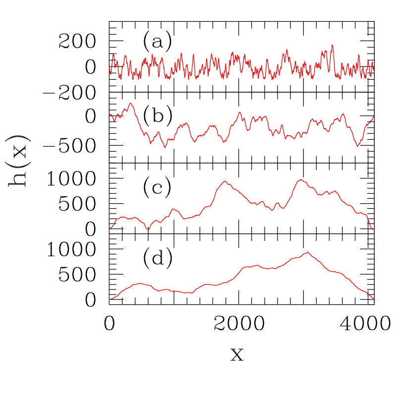
One can have a quantitative understanding of the trends shown in Fig. 1, with the help of wavelet transforms. The corresponding results are displayed in Figure 2, where the horizontal axis is in units of inverse length scale, or “wavenumber” $k\equiv 1/a$. From scaling arguments Simonsen et al. (1998), the averaged wavelet coefficients $W[h](k)$ for a self-similar profile are expected to vary as

$$W[h](k)\sim k^{-[(1/2)+\zeta]}\quad.$$ (8)

A least-squares fit of a power-law dependence to the artificial-profile data for $64\leq k\leq 4096$ gives $\zeta=1.25(1)$. Such a central estimate and its uncertainty are both in line with corresponding results for $0<\zeta<1$ Simonsen et al. (1998).

One sees that for BN data, $\zeta\simeq 1.25$ holds only up to a crossover scale, which (as argued above) increases with $\kappa$. This is illustrated in the inset of Fig. 2, where a section, with $1/32$ of the full length of the ragged $\kappa=1.0$ interface of Fig. 1 (a), is examined. On this scale, the profile is indeed much smoother than its parent.

A fit of $64\leq k\leq 4096$ data for $\kappa=10.0$ results in $\zeta=1.19(3)$. This can be compared, e.g., with finite-size scaling estimates via Eq. (7) for the present model with $\kappa=1.0$, and a sequence of $400\leq L\leq 1200$ with $O(10^{6})$ configurations each, for which one quotes $\zeta=1.24(1)$ de Queiroz (2005a). Eq. (6) reminds one that the latter method only considers fluctuations on short scales, thus in the present case it rightly captures the persistent behavior characteristic of that limit (at the expense of not being sensitive to the different trends that dominate the picture at larger scales).

Figure 2: (Color online) Double-logarithmic plot of averaged wavelet coefficients against wavenumber $k$. Symbols joined by continuous lines: wavelet transform of interface roughness data from two-dimensional BN simulation (interface dimensionality $d^{\prime}=1$). $L=4096$, $10^{5}$ samples, with varying surface tension $\kappa$ (see Eq. (1)). Crosses: wavelet transform of synthetic profile with Hurst exponent $\zeta=1.25$. $L=4096$, $10^{3}$ samples. Continuous line at bottom right has slope $-1.75$. Inset: section of length $L^{\prime}=128$ of typical profile for $\kappa=1.0$, illustrating interface smoothness on short scales (compare Fig. 1 (a)).

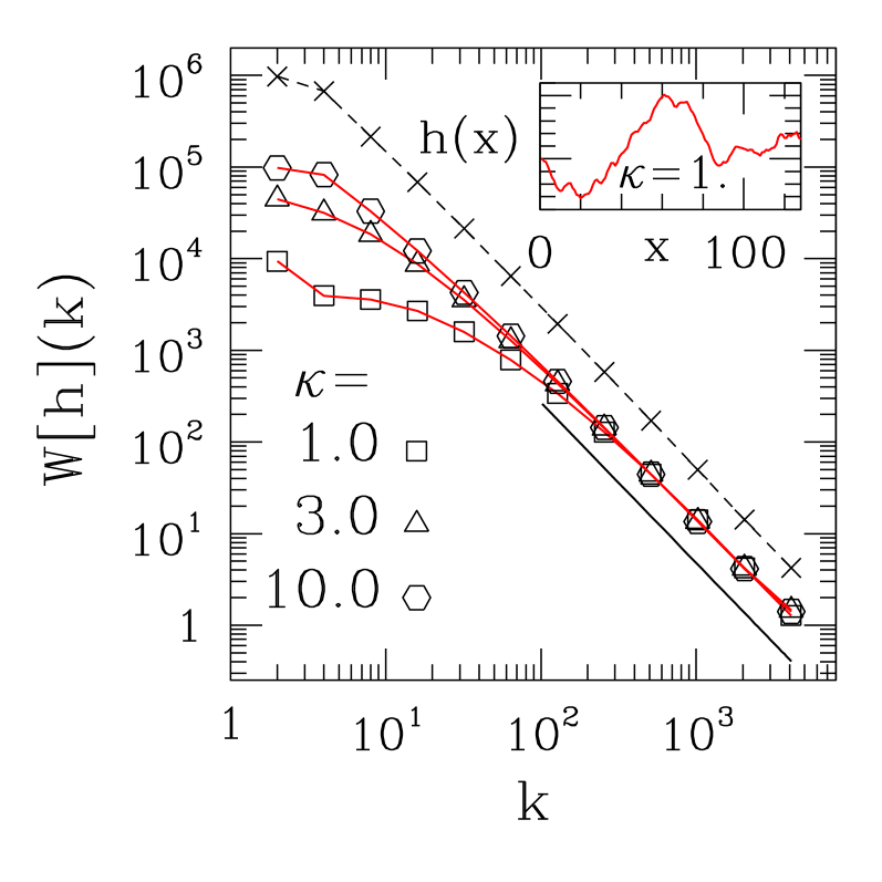
We conclude that the quantitative behavior exhibited by interface roughness in BN is likely to change when studied on varying length scales. Though a regime should exist, which displays close similarity to the Edwards-Wilkinson class of interface evolution problems, this should cross over to a more ragged picture on larger scales (the precise location of such change being determined by the interplay between quenched randomness and surface tension). Wavelet transforms are thus a particularly suitable method for the study of this problem, on account of the equal access that is provided to multiple length scales.

IV time series and power spectra

IV.1 Introduction

As explained above, owing to the assumed linear increase of applied field with time (in analogy with experimental setups), we shall express time in units of $H$ as given in Eqs. (1) and (2).

Initially we consider the adiabatic limit of very slow driving.

In experiment, the integrated signal $\int_{\Delta t}V(t)\,dt$ is proportional to the magnetization change (number of upturned spins) during the interval $\Delta t$. In the adiabatic approximation, a box-like shape is implicitly assumed for each avalanche (i.e. details of the internal structure of each peak, as it develops in time, are ignored, on account of its duration being very short), thus the instantaneous signal intensity (spike height) is proportional to the corresponding avalanche size.

As the signal is intermittent, there are significant periods (waiting times, $WT$) of no activity at all. Waiting time distributions for the adiabatic regime were examined in Ref. de Queiroz (2005b). These were found to be rather flat, apart from (i) a sharp cutoff at the high end (related to the finite cutoff in the avalanche size probability distribution), and (ii) a number of peaks concentrated in a somewhat narrow region, which are associated to very frequent and small, spatially localized (i.e., non-critical) events involving typically $N=1-10$ sites de Queiroz and Bahiana (2001).

We investigate the auto-correlations of two quantities, namely waiting times ($WT$), and avalanche sizes (i.e., BN spike voltages $V$). For $X=WT,\,V$ we calculate normalized, two-time connected correlations, averaged over $t$:

$$G_{X}(\tau)\equiv\frac{\langle X(t)\,X(t+\tau)\rangle_{t}}{\langle X(t)\rangle^{2}_{t}}-1\ .$$ (9)

For a system with $L=400$, we have generated $2\times 10^{4}$ distinct time series of BN events. It is known Urbach et al. (1995) that, on account of the demagnetizing factor, size-size correlations are negative at short times, and decay with a characteristic relaxation time which (for this system size, and for the values of physical parameters used here), is $\tau_{0}\simeq 0.14$ de Queiroz (2005b). Thus, for each sample we calculated correlations in the range $0\leq\tau\leq R$, $R=1.2$, by scanning moving “windows” of width $R$ along an interval of width $10R$. In preparation for ulterior wavelet analysis, the results were binned into $N=1024$ equal-width bins. Our results are depicted in Fig. 3.

Figure 3: (Color online) Waiting-time (WT) and size correlations (see Eq. (9)) against “time” in the adiabatic regime, for system with $L=400$, $2\times 10^{4}$ samples. Inset: absolute values of $G_{X}(\tau)$ on semi-logarithmic plot, same data range as in main Figure.

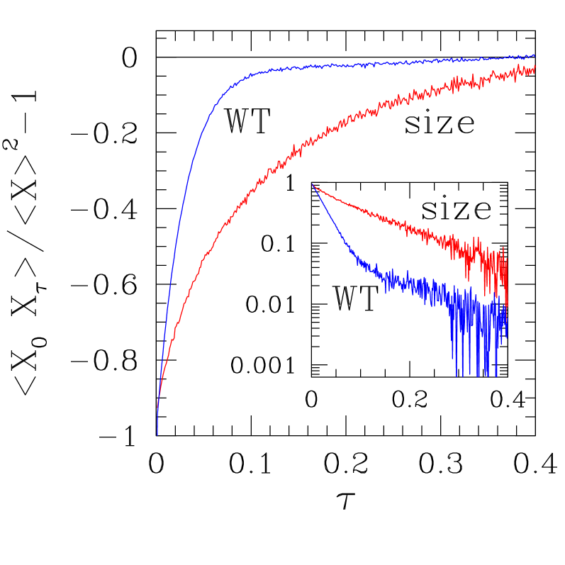
The exponential behavior of size data, noted earlier Urbach et al. (1995); de Queiroz (2005b), is clearly discernible in the Figure even for $\tau\gtrsim 0.3$, by which stage the signal-to-noise ratio has dipped to something close to unity. Waiting-time correlations initially seem to follow a similar exponential trend (with a time constant $\simeq 1/4$ that for their size counterpart); however, a sharp “shoulder” develops at $\tau\approx 0.1$, signalling an abrupt end to the exponential regime. This indicates that negative waiting-time and size correlations have differing underlying causes.

IV.2 Waiting-time correlations

Indeed, in calculating the correlations shown in Fig. 3, the time separation $\tau$ between any two waiting times is considered to be the separation between their respective starting moments (the same is done for size correlations, but it turns out to be of no further consequence, as avalanches are instantaneous in the adiabatic regime). This implies that the minimum separation between two waiting times is the extent of the shortest of the two. Therefore, an effect arises at very short times $\tau$, which is the analogue of hard-core repulsion for stoichiometric problems in real space. Since the distribution of waiting times is flat on a logarithmic scale de Queiroz (2005b) (thus $P(WT)\sim 1/WT$ on a linear scale), and assuming waiting times to be uncorrelated (to be checked below), Eq. (9) gives $|G_{WT}(\tau)|\approx 1-a\,\tau\simeq\exp(-a\tau)$ for $\tau\to 0$.

In order to eliminate this artifact, we then decided to index waiting times simply by their order of occurrence, thus (with $j$, $k$ nonnegative integers)

$$G^{\,\prime}_{WT}(j)=\frac{\langle WT(k)\,WT(k+j)\rangle_{k}}{\langle WT(k)\rangle_{k}^{2}}-1\ .$$ (10)

In analogy with our earlier procedure, correlations were accumulated for $j=1,\dots\,,N$ ($N=1024$) by generating $20$ independent series of $10N$ consecutive events; for each series we scanned moving “windows”, each comprising $N+1$ events, i.e., $N$ waiting times. This time, the result was essentially flat noise, with no apparent short-time structure (see inset in Figure 4 below). Therefore, further characterization must proceed via spectral analysis. We briefly recall how this can be done using wavelets.

Assume one has $1/f^{\alpha}$ noise. One calculates and wavelet-transforms the corresponding ensemble-averaged autocorrelations, and then translation-averages the resulting coefficients at each scale. Denoting the set of averaged wavelet coefficients by $\{W[g](T)\}$, where $\{T\}$ stands for the hierarchical set of wavelet timescales, and changing the independent variable to “frequency” $f=1/T$, one expects from scaling Simonsen et al. (1998); Schmittbuhl et al. (1995):

$$W[g](f)\sim f^{-\alpha}\quad.$$ (11)

For $\alpha>1$ this is derived immediately from Eq. (8), plus the exponent relation $\alpha=1+2\zeta$ Rosso et al. (2003a); de Queiroz (2005a). Though for $0\leq\alpha\leq 1$ the scaling of cumulants of the noise distribution differs from that for $\alpha>1$, the basic scaling properties underlying Eq. (11) remain valid Antal et al. (2002).

Eq. (11) can be tested with pure $1/f^{\alpha}$ noise via the usual procedure of first producing a sequence of Gaussian white noise, Fourier-transforming that sequence, multiplying the Fourier components by $f^{-\alpha/2}$ and then inverting the Fourier transform Antal et al. (2001, 2002). The resulting sequence is pure $1/f^{\alpha}$ noise. An example with $\alpha=1/2$ is shown in Figure 4 below.

Figure 4: (Color online) Double-logarithmic plot of averaged wavelet coefficients against frequency $f$. Squares: wavelet transform of waiting-time autocorrelation data from two-dimensional BN simulation in the adiabatic regime, calculated according to Eq. (10). $L=400$, $20$ independent series of $10\times 1024$ waiting times. Crosses: wavelet transform of autocorrelations for synthetic $1/f^{\alpha}$ noise, $\alpha=1/2$, $L=4096$, $5\times 10^{3}$ samples. A least-squares fit of $16<f<1024$ data gives $\alpha=0.51(1)$. Continuous line has slope $-1/2$. Inset: waiting-time correlations from BN simulation, calculated according to Eq. (10).

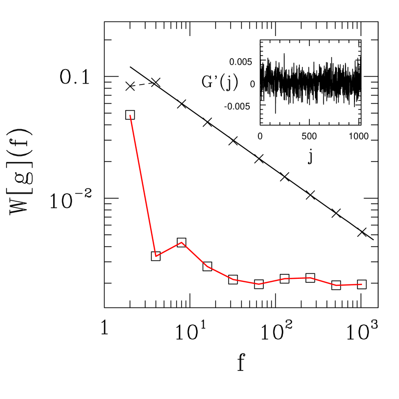
Our results for BN are shown in Fig. 4. Apart from the lowest frequency scale (which is not expected to fall in line with the rest, as it represents the most smoothed-out behavior Press et al. (1992)), the flatness of the averaged coefficients against varying scales strongly indicates that $\alpha=0$ (white noise), i.e., waiting times are indeed uncorrelated.

The sequences of waiting-time correlation data of course need not be periodic. However, as seen above, they behave as random noise. Contrarily to, e.g., generalized brownian-motion profiles, such data are non-cumulative (i.e., they are not constrained in the fashion of consecutive positions of a random-walker, which cannot differ by more than one step length). Thus, the periodic boundary conditions implicit in the wavelet transform are not expected to introduce significant distortions in their analysis.

IV.3 Size correlations: adiabatic regime

We now turn to the treatment of voltage data. For the adiabatic version of the interface model, of course only inter-avalanche voltage correlations can be evaluated. As mentioned above, the data in Fig. 3 are very well fitted by an exponential, with a “loading time” $\tau_{0}=0.14(1)$. One then expects the Fourier power spectrum to be essentially flat for $f\ll\tau_{0}^{-1}$, and to behave as $1/f^{2}$ for $f\gg\tau_{0}^{-1}$. This has indeed been found, e.g., in ref. de Queiroz and Bahiana (2001).

The correlations to be wavelet-transformed are non-periodic and follow a clear baseline trend, therefore one needs to assess and eliminate potential distortions caused by: (i) using a periodic wavelet basis, and (ii) the baseline trend itself.

In Fourier analysis, the standard way to deal with (i) is by zero-padding a region around the function to be transformed Press et al. (1992). However, zero-padding does not work well when the function varies by orders of magnitude between the extremes of the interval Press et al. (1992), as is the case here where only fluctuations are left at the upper end. Techniques have been developed to remove the effects of periodic boundary conditions from wavelet transforms (i.e., to consider “wavelets on the interval”) Freedman and Press (1996). These have very recently been translated into published computer code Press et al. (2007), restricted to the Daub4 class. In the following, motivated especially by the need to address point (ii), we propose a simplified approach based on detrending ideas. Combinations of wavelet decomposition and detrending have been investigated Manimaran et al. (2005); however, the averaged coefficient analysis which is our main concern here has not been considered, except for some very simple cases (linear and quadratic drift Simonsen et al. (1998)).

We first illustrate how the averaged coefficients are affected by an overall exponential trend. Using the periodic Daub4 basis, we wavelet-transformed the size-correlation fitting function, $G_{V}^{\,\rm fit}(\tau)=-\exp(-\tau/\tau_{0})$. From Eq. (4), one has:

$${\cal W}[G_{V}^{\,\rm fit}](a,b)=\frac{1}{\sqrt{a}}\int_{-\infty}^{\infty}\psi_{a;b}(x)\,e^{-x/\tau_{0}}\,dx\ .$$ (12)

By changing variables, Eq. (12) turns into:

$${\cal W}[G_{V}^{\,\rm fit}](a,b)=\sqrt{a}\,e^{-b/\tau_{0}}\int_{-\infty}^{\infty}\psi_{1;0}(x^{\prime})\,e^{-ax^{\prime}/\tau_{0}}\,dx^{\prime}\ .$$ (13)

The first $p=M/2$ moments (starting at zeroth order) of Daubechies wavelets of order $M$ vanish Press et al. (1992). Thus, for $M=4$ as is the case here, Taylor-expanding the exponential in the integrand of Eq. (13), one sees that the lowest-order non-zero term is proportional to $a^{5/2}$, i.e.,

$${\cal W}[G_{V}^{\,\rm fit}](a,b)\propto{a}^{5/2}\,e^{-b/\tau_{0}}+{\cal O}({a}^{7/2})\ \ .$$ (14)

We evaluated $G_{V}^{\,\rm fit}(\tau)$ at $N=4096$ equally-spaced points in the interval $0<\tau<1.5$, and wavelet-transformed it. For each hierarchical level $j>2$, we plotted all $2^{j}$ wavelet coefficients, and found that they fall on the exponential-decay pattern of the original function, and (at the $j$–th hierarchical level) are proportional to $2^{-5j/2}$, both features as predicted in Eq. (14), except for the last two (“wraparound” coefficients Press et al. (1992)). In order to fulfill the implicitly assumed periodicity of the original function, the latter coefficients take values $\sim 10^{j}$ larger than the last preceding one (see an example for $j=5$ in the inset of Fig. 5). Including these data in the coefficient-averaging procedure would introduce sizeable distortions (we did it, and found that the coefficients thus averaged behave as $1/f$, which is in clear disagreement with the prediction of Eq. (14) of a scaling power $5/2$).

To correct this artifact, we discarded the wraparound coefficients from the averaging procedure. Similar procedures have been adopted elsewhere Manimaran et al. (2005). As can be seen in Fig. 5, this was enough to restore the expected behavior. Thus, point (i) above has been dealt with.

Figure 5: (Color online) Main diagram: double-logarithmic plot of averaged wavelet coefficients against frequency $f$. Squares: wavelet transform of $N=4096$ points of fitting function for size correlations, $G_{V}^{\,\rm fit}(\tau)$, for $0<\tau<1.5$. At each hierarchical level $j>2$, the last two coefficients were omitted from the averages (see text). Continuous straight line has slope $-5/2$. Inset: semilogarithmic plot of (absolute value of) all $32$ wavelet coefficients ${\cal W}[G_{V}^{\,\rm fit}](a,b)$ [denoted by $W_{a}(b)$] against translation parameter $b$, at hierarchical level $j=5$.

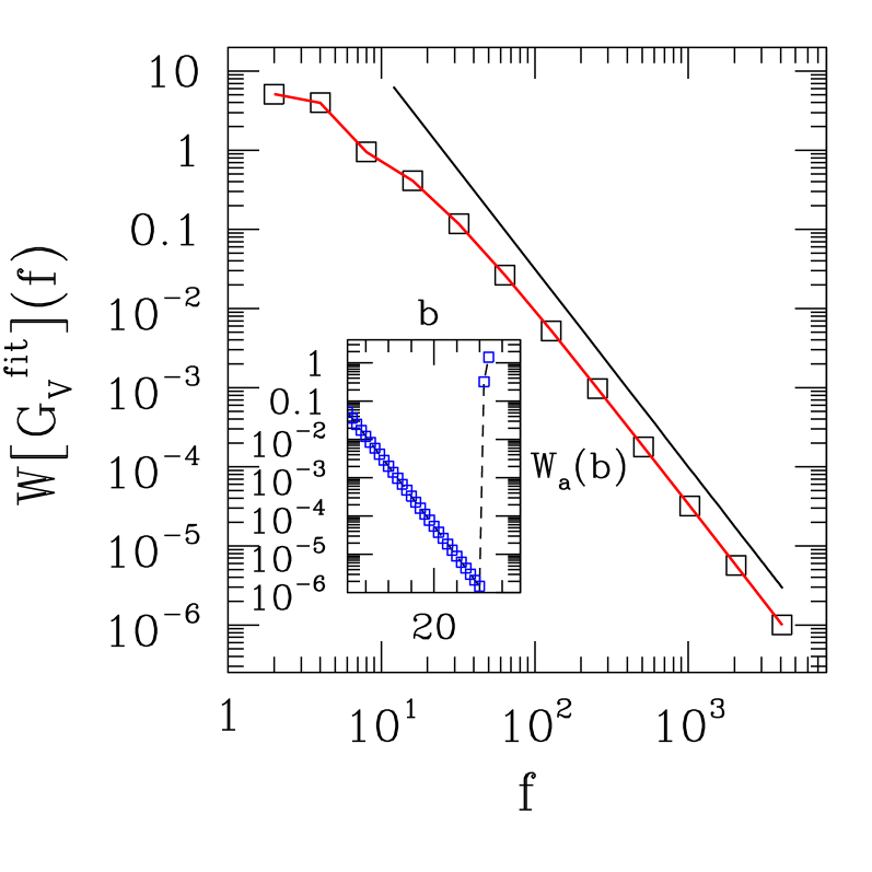
We also wavelet-transformed $G_{V}^{\,\rm fit}(\tau)$ using the periodic Daub12 basis. As expected, the coeficients behaved approximately as ${a}^{13/2}\,e^{-b/\tau_{0}}$. The last four coefficients at each hierarchical level showed considerable increase against the exponential-decay pattern (as opposed to the last two for Daub4). In summary, as regards point (ii) we have shown that the most prominent feature of the wavelet transform (in the context of average wavelet coefficient scaling), namely the Hurst-like exponent, of such a smooth function as the exponential fit is in fact basis-dependent.

Thus, our simulational data must be detrended in order to eliminate distortions coming from the smooth baseline, which risk contaminating all scales. We did this by first subtracting the dominant exponential behavior given by $G_{V}^{\,\rm fit}(\tau)$; for further refinement, we then removed some remaining non-monotonic mismatch via least-squares fit of a secondary adjusting function $f(\tau)$ (a fourth-degree polynomial enveloped by a single exponential), so $G_{V}^{\,\rm d}(\tau)=G_{V}(\tau)-G_{V}^{\,\rm fit}(\tau)-f(\tau)$. The result of wavelet-transforming the fully detrended correlations is depicted in Fig. 6, while the corresponding raw (detrended) data are shown in the inset of the same Figure (together with $f(\tau)$, so one can have a quantitative estimate of how far the single-exponential fit goes to describe the un-detrended data). Note that $f(\tau)$ has significant smooth variations on scales of $\delta\tau=0.05$ or longer, which translate into wavevectors $k\lesssim 32$. We have wavelet-transformed partially-detrended data [ i.e., without subtracting $f(\tau)\,$]. The respective averaged wavelet coefficients are $\sim 10$ times larger than those for the fully-detrended curve for $k\leq 16$, and fall fast for increasing $k$: at $k=64$ the ratio is $1.4$, and for $k>64$ both sets coincide to within less than $1\%$. So, failing to subtract $f(\tau)$ introduces artificially large coefficients at large scales, which are not noise-related.

Note that similar remarks apply here as in the earlier case of waiting-time correlations, namely, since $G_{V}^{\,\rm d}(\tau)$ is essentially noise around a horizontal baseline, the periodic boundary conditions implicit in the wavelet transform must not imply any significant distortion in our results.

Figure 6: (Color online) Double-logarithmic plot of averaged wavelet coefficients against frequency $f$. Squares: wavelet transform of detrended size autocorrelation data, $G_{V}^{\,\rm d}(\tau)$ from two-dimensional BN simulation in the adiabatic regime. $L=400$, $2\times 10^{4}$ samples. Inset: full lines: fully-detrended size correlations from BN simulation; dashed line: secondary adjusting functon $f(\tau)$ (see text).

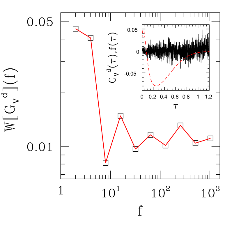
The results exhibited in the main diagram of Fig. 6 strongly indicate that the detrended size correlations behave as $1/f^{0}$ (white) noise. We defer discussion of this until the next Subsection, where departures from the adiabatic regime are investigated.

IV.4 Size correlations: finite driving rate

In order to discuss intra-avalanche correlations, one must introduce a finite driving rate de Queiroz and Bahiana (2001); Tadić (1999); White and Dahmen (2003), so separate events within the same avalanche can be ascribed to different instants in time. In line with standard practice Tadić (1999); Perković et al. (1999); Tadić (2000); Tadić and Nowak (2000); Kuntz and Sethna (2000) our basic time unit is one lattice sweep, during which the external field is kept constant, and all spins on the interface are probed sequentially as described above. In the adiabatic regime, the external field is kept constant for the whole duration of an avalanche, i.e. for as many sweeps as it takes until no unstable sites are found along the interface. At finite driving rates, the field is increased by a fixed amount, henceforth denoted $\Delta$, at the start of each sweep while an avalanche is taking place. Eventually, no more unstable sites will be left, and then one proceeds as in the adiabatic regime, increasing the field by the minimum amount $\delta H$ necessary to start a new avalanche. In these “real” time units, the waiting time between the end of one event and the start of the next is then $\delta H/\Delta$; however, in order to produce meaningful comparisons, especially between data acquired in the adiabatic and non-adiabatic regimes, it will be useful to keep referring to the “absolute” scale given by the applied field $H$ itself, which unequivocally locates events along the hysteresis cycle.

As $\Delta$ grows, the intermittent character of events is gradually lost as more and more avalanches coalesce de Queiroz and Bahiana (2001), and one eventually crosses over to a regime in which the interface is fully depinned, i.e. it moves at non-zero average speed.

Figure 7: (Color online) Normalized two-time correlations (averaged over $t$) $\langle V(t)\,V(t+\tau)\rangle/\langle V(t)\rangle^{2}-1$ from two-dimensional BN simulation, for system with $L=400$, and driving rates $\Delta$ as given in key to symbols ($\Delta=0$ corresponds to adiabatic limit). “Time” is given in applied field units, i.e. “absolute” scale (see text).

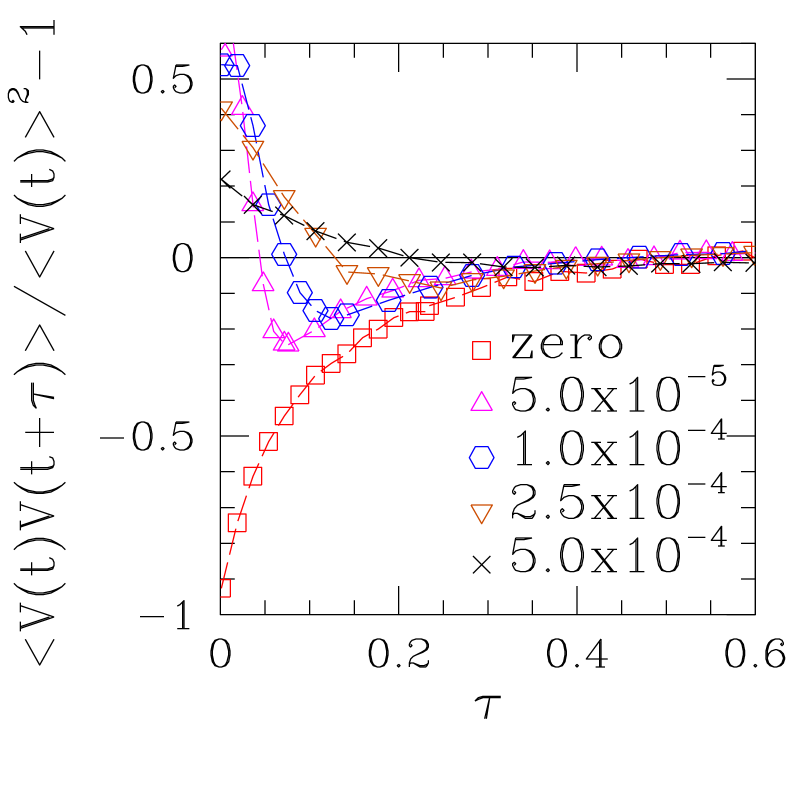
In Fig. 7 we show autocorrelations for driving rates still within the intermittent regime, compared with those for the adiabatic limit. The most significant change upon increasing $\Delta$ is the effective loss of negative short-time correlations. In fact, this represents an excess of positive intra-avalanche contributions, on top of the negative inter-avalanche terms (and some intra-avalanche ones as well) which still exist for non-zero $\Delta$ (on account of the demagnetizing factor). Positive reinforcements arise mostly because, when many sites are overturned during one lattice sweep, that same number of new sites will be probed by the interface. For each new site, the quenched randomness term in Eq. 1 may, or may not, contribute to further motion with roughly equal chances. By contrast, at a site which remains pinned during one sweep, the interface stands fewer chances of getting unstuck, as the contribution from the randomness term is kept constant; depinning of such a site is more likely to happen if the field is substantially increased, i.e., during a subsequent avalanche.

We detrended the $\Delta\neq 0$ data of Fig. 7 by similar procedures to those used earlier for $\Delta=0$. The main difference was that detrending was done in a single stage, fitting $f(\tau)$ described in Subsec. IV.3 to the raw data, and then subtracting the least-squares-fit from the original data. The results of wavelet-transforming the detrended data are shown in Figure 8.

Figure 8: (Color online) Double-logarithmic plot of averaged wavelet coefficients against frequency $f$, from wavelet transform of detrended size autocorrelation data, $G_{V}^{\,\rm d}(\tau)$, for two-dimensional BN simulations of system with $L=400$, and assorted driving rates $\Delta$. Key to symbols is the same as in Fig. 7 ($\Delta=0$ corresponds to adiabatic limit). Frequency is given in inverse applied field units, i.e. “absolute” scale (see text). Plots successively shifted downward by a factor of $10$ on vertical scale, to avoid superposition. Straight line segments mark subsets of $\Delta\neq 0$ regime where approximate $1/f^{1.5}$ behavior holds.

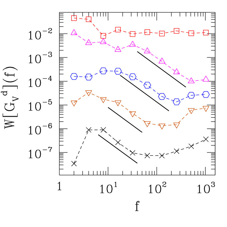
One can see that, as opposed to the adiabatic regime, data for finite driving rates clearly exhibit a downward trend for a range of intermediate frequencies, spanning 3-4 hierarchical levels, and which is characterized by an approximate $1/f^{1.5}$ behavior (the straight line segments in the Figure have slope $-1.5$). Furthermore, with the “absolute” frequency $f$ given in inverse applied field units, and $\Delta$ given in units of applied field change per unit time, dimensional arguments show that $f^{\prime}\equiv f\,\Delta$ is the “natural” frequency variable (i.e., inverse “real” time). This is shown more clearly on a scaling plot, Figure 9, where use of $f^{\prime}$ as the independent variable causes the $1/f^{1.5}$ sections of all $\Delta\neq 0$ data to collapse.

Figure 9: (Color online) Double-logarithmic scaling plot of averaged wavelet coefficients against “natural” frequency $f^{\prime}\equiv f\,\Delta$, from wavelet transform of detrended size autocorrelation data, $G_{V}^{\,\rm d}(\tau)$, for two-dimensional BN simulations of system with $L=400$, and assorted driving rates $\Delta\neq 0$. Key to symbols is the same as in Figs. 7 and 8. Full straight line has slope $-1.5$ .

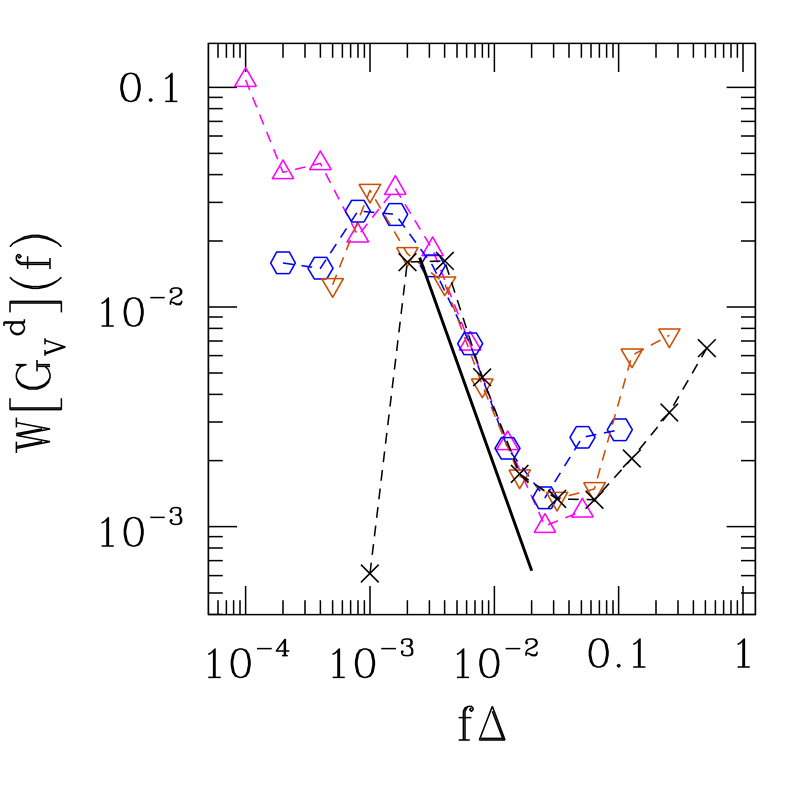
Given that, in these slow- (but non-adiabatic) driving regimes, avalanche coalescence comprises only a small fraction of events de Queiroz and Bahiana (2001), one can say that approximately the same sequence of avalanches occurs for all $\Delta$ investigated here, only at different “real” paces. Since the “real” time interval between consecutive avalanches is $\delta h/\Delta$, and assuming $\delta h$ to be the same, for different values of $\Delta$, between two given avalanches (for the reasons just mentioned), one sees that inter-avalanche correlations will shift to higher “real” frequencies as $\Delta$ grows. On the other hand, within a given avalanche, two sub-events separated by a given number of lattice sweeps are (by definition used in the simulation) separated by the same “real” time interval, thus their correlations are not shifted in “real” frequency for varying $\Delta$. Therefore we conclude that the collapsing sections of the scaling plot correspond mainly to intra-avalanche correlations.

First-order (Haar) spectra of experimental BN data show that, for Fe₂₁Co₆₄B₁₅ the high-frequency section falls initially as $f^{-1.2}$, and then crosses over to $f^{-1.9}$, while for Fe Si the decay is with $f^{-1.65}$ Petta et al. (1998a, b). Though the exponent values in both cases are not too dissimilar to the one found here, analysis of higher-order spectra O’Brien and Weissman (1994) leads to a more nuanced picture. For Fe₂₁Co₆₄B₁₅, it is found that most of the power in the high-frequency range comes from intra-pulse correlations Petta et al. (1998a), similar to our conclusion above, whereas for Fe Si the conclusion was that the high-frequency power is mainly connected to the inter-pulse sort Petta et al. (1998b). Therefore it would appear that the dynamics of the present model is closer to that of BN in materials like Fe₂₁Co₆₄B₁₅ than in Fe Si.

V Discussion and Conclusions

We have discussed the application of wavelet transforms to the description of both real-space and time-like properties of an interface model, which is used for the description of Barkhausen noise in soft ferromagnets. Most of our calculations involved the scaling properties of positional averages of wavelet coefficients, taken at each hierarchical (size) level, as first proposed in Ref. Simonsen et al., 1998. In some instances we showed that direct analysis of individual coefficients was called for, in order to unravel artificial effects which would otherwise distort our aggregate results.

Here we considered the $d=2$ version of the model (thus the interface dimensionality is $d^{\prime}=1$), mainly in the adiabatic limit of very slow driving, for which the sudden “avalanches” of domain wall motions are considered to occur instantaneously. In Subsection IV.4, we extended our study to finite driving rates, in order to analyze intra-avalanche correlations

Our investigation of real-space aspects consisted in the evaluation of the characteristic interface roughness exponent $\zeta$. On scales shorter than a crossover length (which turns larger as the intensity of surface tension grows), we get $\zeta=1.20(3)$, close to $\zeta=1.24(1)$, derived by other methods for the same model de Queiroz (2005a), and also to assorted estimates for quenched Edwards-Wilkinson systems Leschhorn (1993); Makse and Amaral (1995); Makse et al. (1998); Rosso et al. (2003b), which give $\zeta\simeq 1.25$.

Turning to time series, in Subsection IV.2 we showed that a proper indexation of the sequence of waiting-times between avalanches is crucial, in order to avoid artificial short-time negative correlations. Procedures similar to that used here, namely, indexing waiting times simply by their order of occurrence (instead of using the starting time of each interval), have been used consistently in the context of self-organized criticality scaling Davidsen and Paczuski (2002). Our final result (see Fig. 4) was that the correlations between waiting times are white noise, i.e., these quantities are fully uncorrelated. Going back to the rules of interface motion, and to Eqs. (1) and (2), one sees that this is a signature of the quenched-randomness term $u(x_{i},h_{i})$. This fact is in contrast to the behavior of size correlations, which are strongly influenced by demagnetization Urbach et al. (1995); de Queiroz (2005b).

In Subsection IV.3, we started from the known fact that, in the adiabatic regime, size-size correlations are negative at short times, and decay approximately as an exponential Urbach et al. (1995); de Queiroz (2005b). By direct analysis of (non-averaged) wavelet coefficients, we illustrated practical ways to deal with artifacts introduced by the periodicity of the wavelet basis used. It turned out that the smooth baseline function, to which noise data are fitted, can introduce distortions at all levels of the wavelet transform. Furthermore, such distortions are non-universal in the sense that they depend on the wavelet basis. Thus, in order to obtain meaningful results from averaged wavelet coefficients, one must fully detrend the raw data. Once we did so, we found strong indications that the detrended size correlations behave as white noise (see Fig. 6). This is apparently at odds with earlier (Fourier) power-spectrum results (see, e.g., Ref. de Queiroz and Bahiana, 2001 and references therein), which would lead one to expect $1/f^{2}$ behavior, at least for high frequencies. However, the derivation of the latter result (e.g., by direct integration) fully takes into account the exponential baseline shape, thus one is referring to a different object. Here, as explained above, we are dealing with detrended data.

Finally, in Subsection IV.4, we considered size correlations against time in non-adiabatic regimes (but well within the driving-rate range where intermittency still holds de Queiroz and Bahiana (2001)). For driving rates $\Delta$ spanning one order of magnitude, we found rather well-defined frequency intervals for which detrended correlations behave as $f^{-\alpha}$, $\alpha\approx 1.5$, By changing variables from “absolute” to “natural” frequency, we found that said intervals collapse together, which indicates that they pertain to intra-avalanche correlations. Rather than attaching much significance to the numerical value of the power-law exponent (since the shortness of the interval along which such behavior holds prevents one from doing so), one must emphasize the good degree of curve collapse exactly in that section, and only there. This indicates that this section is the "special" one, i.e. it corresponds to the frequency range along which universal (driving-rate independent) properties hold. Furthermore, our considerations leading to the conclusion that such scaling behavior reflects intra-avalanche correlations are completely independent of the analysis of higher-order power spectra experimental data, carried out in Refs. Petta et al., 1998a, b, and which leads to the very same conclusion as regards BN in samples of Fe₂₁Co₆₄B₁₅.