Hydrodynamic Theory of Granular Solids:
Permanent, Transient and Granular Elasticity

Yimin Jiang Theoretische Physik, Universität Tübingen,72076 Tübingen, Germany Central South University, Changsha 410083, China    Mario Liu Theoretische Physik, Universität Tübingen,72076 Tübingen, Germany
Abstract

Although fully elastic when static, granular media become transiently elastic when being slowly sheared – during which both the elastic energy and stress relax. Starting from this observation, we cogently derive the framework for granular hydrodynamics, a set of differential equations consistent with general principles of physics, especially reversible and irreversible thermodynamics. In addition, an expression for the granular elastic energy is reviewed and further discussed.

pacs:
81.40.Lm, 83.60.La, 46.05.+b, 45.70.Mg

I Introduction

In granular media, although the grains roll and slide, in addition to being compressed and sheared, only the latter, the deformation of the grains, leads to reversible energy storage that sustains a static, elastic stress, while rolling and sliding heats up the system. The granular strain field εijsubscript𝜀𝑖𝑗\varepsilon_{ij}, therefore, has two contributions, an elastic one uijsubscript𝑢𝑖𝑗u_{ij} accounting for deformation of the grains, and a plastic one pijsubscript𝑝𝑖𝑗p_{ij} for the rest, where εij=uij+pijsubscript𝜀𝑖𝑗subscript𝑢𝑖𝑗subscript𝑝𝑖𝑗\varepsilon_{ij}=u_{ij}+p_{ij}. The elastic energy w(uij)𝑤subscript𝑢𝑖𝑗w(u_{ij}) is a function of uijsubscript𝑢𝑖𝑗u_{ij}, not of εijsubscript𝜀𝑖𝑗\varepsilon_{ij}, and the elastic contribution to the stress σijsubscript𝜎𝑖𝑗\sigma_{ij} is given as πij(uij)w/uijsubscript𝜋𝑖𝑗subscript𝑢𝑖𝑗𝑤subscript𝑢𝑖𝑗\pi_{ij}(u_{ij})\equiv-\partial w/\partial u_{ij}. With σij=πijsubscript𝜎𝑖𝑗subscript𝜋𝑖𝑗\sigma_{ij}=\pi_{ij} in statics, stress balance jσij=0subscript𝑗subscript𝜎𝑖𝑗0\nabla_{j}\sigma_{ij}=0 may be closed with πij=πij(uij)subscript𝜋𝑖𝑗subscript𝜋𝑖𝑗subscript𝑢𝑖𝑗\pi_{ij}=\pi_{ij}(u_{ij}) and uniquely determined employing appropriate boundary conditions J-L ; ge . Because the plastic part of the strain needed for arriving at a given stress state is quite irrelevant for its determination, one may with certain justification consider static granular media, say a sand pile at rest, as fully elastic.

If this sand pile is perturbed by periodic tapping, circumstances change qualitatively. Its conic form will then degrade until the surface becomes flat. This is because part of the grains in the pile loose contact with each other temporarily, during which their deformation decreases. This implies a relaxing elastic strain uijsubscript𝑢𝑖𝑗u_{ij}, and correspondingly, smaller elastic energy w(uij)𝑤subscript𝑢𝑖𝑗w(u_{ij}) and static stress πij(uij)subscript𝜋𝑖𝑗subscript𝑢𝑖𝑗\pi_{ij}(u_{ij}). Since the sand pile is no longer able to sustain static stresses, it is now a transiently elastic system, same as polymers – though the respective microscopic mechanisms are of course very different: temporary unjamming and rearrangement of the grains versus slow disentanglement of polymer strands. Note that flattening a sand pile implies sizable granular rearrangement, requiring a considerable portion of plastic strain pijsubscript𝑝𝑖𝑗p_{ij}.

Quantifying the random motion of the grains as granular temperature Tgsubscript𝑇𝑔T_{g}, we may take the relaxation time τ𝜏\tau of the elastic strain uijsubscript𝑢𝑖𝑗u_{ij} as a function of Tgsubscript𝑇𝑔T_{g}, with τ(Tg)𝜏subscript𝑇𝑔\tau(T_{g})\to\infty for Tg0subscript𝑇𝑔0T_{g}\to 0. For vanishing Tgsubscript𝑇𝑔T_{g}, there is no strain relaxation, the deformation of the grains are maintained, the sand pile keeps its conic shape, and the system is elastic. For finite Tgsubscript𝑇𝑔T_{g}, the elasticity turns transient, with uijsubscript𝑢𝑖𝑗u_{ij}, πij(uij)subscript𝜋𝑖𝑗subscript𝑢𝑖𝑗\pi_{ij}(u_{ij}) and w(uij)𝑤subscript𝑢𝑖𝑗w(u_{ij}) relaxing.

When granular media are being slowly sheared, circumstances are similar. In addition to moving with the large scale velocity visubscript𝑣𝑖v_{i}, the grains also move and slip in deviation of it. This allows temporary, partial unjamming, and implies a finite Tgsubscript𝑇𝑔T_{g}, both again lead to transient elasticity. Since Tgsubscript𝑇𝑔T_{g} is not always an externally imposed parameter, as with tapping, but frequently internally produced, especially by shear flows, it is an independent variable of the granular hydrodynamic theory, to be accounted for by its own equation of motion. More specifically, the production of Tgsubscript𝑇𝑔T_{g} by shear flows should have great similarities to viscous heat production in normal fluids.

Granular media has different phases that, in dependence of the grain’s ratio of deformation to kinetic energy, may loosely be referred to as gaseous, liquid and solid. Moving fast and being free most of the time, the grains in the gaseous phase have much kinetic, but next to none elastic, energy Haff . In the denser liquid phase, say in chute flows, there is less kinetic energy, more deformation, and a rich rheology that has been scrutinized recently chute . In granular statics, with the grains deformed but stationary, the energy is all elastic. This state is legitimately referred to as solid because static shear stresses are sustained. If granular solid is slowly sheared, the predominant part of the energy remains elastic. As discussed, the system is transiently elastic, or quasi-solid. In this paper, we focus on the last two cases, and for simplicity refer to both as the solid granular phase.

The transition between permanent and transient elasticity is a crucial key to understanding granular solids. And remarkably, it is as input quite sufficient for a formal and cogent derivation of the framework for granular solid hydrodynamics – if one takes careful notice of all general principles of physics, especially symmetry and thermodynamic considerations. This is the first part of the present paper. The second part deals with an concrete expression for the granular elastic energy, how this expression is supported by extensive experimental data from granular statics. This is important because general principles only confines the structure of the hydrodynamic theory – they yield a framework into which many different theories fit. The three sets of differential equations given below need the input of specific expressions for the thermodynamic energy and the transport coefficients. Only when their functional dependence on the thermodynamic variables is given, do the theories attain predictive power.

In the following, we first recall the hydrodynamic theory of permanent and transient elasticity, in § II.1 and § II.2; then merge both to form granular hydrodynamics, in § II.3. All equations in these three subsections are valid irrespective what form the energy w𝑤w has. A specific energy density suitable for granular media is then reviewed and further discussed in § III.

In an accompanying paper JL3 , we compare hypoplasticity Kolym , a state of the art engineering model on the behavior of granular solids, with granular solid hydrodynamics as derived here, and specified using the elastic energy of § III.

II Elasticity Theory

II.1 Permanent Elasticity

The conserved, thermodynamic energy density w𝑤w of solids is a function of the symmetric strain field uij=ujisubscript𝑢𝑖𝑗subscript𝑢𝑗𝑖u_{ij}=u_{ji}, and of the densities of entropy s𝑠s, mass ρ𝜌\rho, momentum 𝒈𝒈\boldsymbol{g}. So we write (neglecting gravity)

dw=Tds+μdρ+vidgiπijduij,d𝑤𝑇d𝑠𝜇d𝜌subscript𝑣𝑖dsubscript𝑔𝑖subscript𝜋𝑖𝑗dsubscript𝑢𝑖𝑗{\rm d}w=T{\rm d}s+\mu{\rm d}\rho+v_{i}{\rm d}g_{i}-\pi_{ij}{\rm d}u_{ij}, (1)

denoting T(s,ρ,uij)w/s𝑇𝑠𝜌subscript𝑢𝑖𝑗𝑤𝑠T(s,\rho,u_{ij})\equiv\partial w/\partial s, μ(s,ρ,gi,uij)w/ρ𝜇𝑠𝜌subscript𝑔𝑖subscript𝑢𝑖𝑗𝑤𝜌\mu(s,\rho,g_{i},u_{ij})\equiv\partial w/\partial\rho, viw/gi=gi/ρsubscript𝑣𝑖𝑤subscript𝑔𝑖subscript𝑔𝑖𝜌v_{i}\equiv\partial w/\partial g_{i}=g_{i}/\rho, πij(s,ρ,uij)w/uijsubscript𝜋𝑖𝑗𝑠𝜌subscript𝑢𝑖𝑗𝑤subscript𝑢𝑖𝑗\pi_{ij}(s,\rho,u_{ij})\equiv-\partial w/\partial u_{ij}. The equations of motion for the energy and its variables are

tw+iQi=0,ts+ifi=R/T,formulae-sequence𝑡𝑤subscript𝑖subscript𝑄𝑖0𝑡𝑠subscript𝑖subscript𝑓𝑖𝑅𝑇\displaystyle{\textstyle\frac{\partial}{\partial t}}w+\nabla_{i}Q_{i}=0,\qquad{\textstyle\frac{\partial}{\partial t}}s+\nabla_{i}f_{i}=R/T, (2)
tρ+iji=0,tgi+jσij=0,formulae-sequence𝑡𝜌subscript𝑖subscript𝑗𝑖0𝑡subscript𝑔𝑖subscript𝑗subscript𝜎𝑖𝑗0\displaystyle{\textstyle\frac{\partial}{\partial t}}\rho+\nabla_{i}j_{i}=0,\qquad{\textstyle\frac{\partial}{\partial t}}g_{i}+\nabla_{j}\sigma_{ij}=0, (3)
ddtuijvij+[12iyj+uikjvk+ij]=0,\displaystyle{\textstyle\frac{\rm d}{{\rm d}t}}u_{ij}-v_{ij}+[{\textstyle\frac{1}{2}}\nabla_{i}y_{j}+u_{ik}\nabla_{j}v_{k}+i\leftrightarrow j]=0, (4)

where ddt=t+vkkdd𝑡𝑡subscript𝑣𝑘subscript𝑘{\textstyle\frac{\rm d}{{\rm d}t}}={\textstyle\frac{\partial}{\partial t}}+v_{k}\nabla_{k} and vij12(ivj+jvi)subscript𝑣𝑖𝑗12subscript𝑖subscript𝑣𝑗subscript𝑗subscript𝑣𝑖v_{ij}\equiv\frac{1}{2}(\nabla_{i}v_{j}+\nabla_{j}v_{i}). Expressing conservation laws and entropy production, the first four equations are quite general and shared by all hydrodynamic theories. Alone, they describe normal fluids and represent the simplest hydrodynamic theory. The fifth equation is characteristic of elastic systems, especially ones that break the translational symmetry spontaneously. (More on why Eq (4) must have the above form is given in temmen .) Inserting Eqs (2-4) into the temporal derivative of Eq (1),

tw=Tts+μtρ+vitgiπijtuij,𝑡𝑤𝑇𝑡𝑠𝜇𝑡𝜌subscript𝑣𝑖𝑡subscript𝑔𝑖subscript𝜋𝑖𝑗𝑡subscript𝑢𝑖𝑗\textstyle\frac{\partial}{\partial t}w=T\frac{\partial}{\partial t}s+\mu\frac{\partial}{\partial t}\rho+v_{i}\frac{\partial}{\partial t}g_{i}-\pi_{ij}\frac{\partial}{\partial t}u_{ij}, (5)

and introducing the notations: fiDsubscriptsuperscript𝑓𝐷𝑖f^{D}_{i}, σijDsubscriptsuperscript𝜎𝐷𝑖𝑗\sigma^{D}_{ij}, taking them to be given as

fisubscript𝑓𝑖\displaystyle f_{i} \displaystyle\equiv svifiD,𝑠subscript𝑣𝑖subscriptsuperscript𝑓𝐷𝑖\displaystyle sv_{i}-f^{D}_{i}, (6)
σijsubscript𝜎𝑖𝑗\displaystyle\sigma_{ij} \displaystyle\equiv πijπikujkπjkuiksubscript𝜋𝑖𝑗subscript𝜋𝑖𝑘subscript𝑢𝑗𝑘subscript𝜋𝑗𝑘subscript𝑢𝑖𝑘\displaystyle\pi_{ij}-\pi_{ik}u_{jk}-\pi_{jk}u_{ik} (7)
+(Ts+vigi+μρ+givjw)σijD,𝑇𝑠subscript𝑣𝑖subscript𝑔𝑖𝜇𝜌subscript𝑔𝑖subscript𝑣𝑗𝑤subscriptsuperscript𝜎𝐷𝑖𝑗\displaystyle\quad+(Ts+v_{i}g_{i}+\mu\rho+g_{i}v_{j}-w)-\sigma^{D}_{ij},

we obtain

iQi=i(Tfi+μji+vjσijyjπij)subscript𝑖subscript𝑄𝑖subscript𝑖𝑇subscript𝑓𝑖𝜇subscript𝑗𝑖subscript𝑣𝑗subscript𝜎𝑖𝑗subscript𝑦𝑗subscript𝜋𝑖𝑗\displaystyle\nabla_{i}Q_{i}=\nabla_{i}(Tf_{i}+\mu j_{i}+v_{j}\sigma_{ij}-y_{j}\pi_{ij}) (8)
+fiDiT+σijDvij+yijπijR.superscriptsubscript𝑓𝑖𝐷subscript𝑖𝑇superscriptsubscript𝜎𝑖𝑗𝐷subscript𝑣𝑖𝑗subscript𝑦𝑖subscript𝑗subscript𝜋𝑖𝑗𝑅\displaystyle+f_{i}^{D}\nabla_{i}T+\sigma_{ij}^{D}v_{ij}+y_{i}\nabla_{j}\pi_{ij}-R.

Clearly, one can write the left hand side of Eq (5) as the divergence of something, plus something else that vanishes in equilibrium (because the so-called thermodynamic forces, iT,vijsubscript𝑖𝑇subscript𝑣𝑖𝑗\nabla_{i}T,v_{ij} and jπijsubscript𝑗subscript𝜋𝑖𝑗\nabla_{j}\pi_{ij} do). Therefore, an inviting possibility is to identify the first with the energy flux Qisubscript𝑄𝑖Q_{i}, and the second with the entropy production R𝑅R, a quantity that also vanishes in equilibrium,

Qi=Tfi+μji+vjσijyjπij,subscript𝑄𝑖𝑇subscript𝑓𝑖𝜇subscript𝑗𝑖subscript𝑣𝑗subscript𝜎𝑖𝑗subscript𝑦𝑗subscript𝜋𝑖𝑗\displaystyle Q_{i}=Tf_{i}+\mu j_{i}+v_{j}\sigma_{ij}-y_{j}\pi_{ij}, (9)
R=fiDiT+σijDvij+yijπij.𝑅subscriptsuperscript𝑓𝐷𝑖subscript𝑖𝑇subscriptsuperscript𝜎𝐷𝑖𝑗subscript𝑣𝑖𝑗subscript𝑦𝑖subscript𝑗subscript𝜋𝑖𝑗\displaystyle R=f^{D}_{i}\nabla_{i}T+\sigma^{D}_{ij}v_{ij}+y_{i}\nabla_{j}\pi_{ij}. (10)

This identification is in fact unique. It is easy to verify that, as long as the energy w𝑤w remains general, unspecified, there is no other way to write the left hand side of Eq (5) as the sum of a divergence and an expression that vanishes in equilibrium.

Taking in Eq (10) (iT,vij,jπij)subscript𝑖𝑇subscript𝑣𝑖𝑗subscript𝑗subscript𝜋𝑖𝑗(\nabla_{i}T,v_{ij},\nabla_{j}\pi_{ij}) as the thermodynamic forces, (fiD,σijD,yi)subscriptsuperscript𝑓𝐷𝑖subscriptsuperscript𝜎𝐷𝑖𝑗subscript𝑦𝑖(f^{D}_{i},\sigma^{D}_{ij},y_{i}) as the fluxes, and forming each into a 12-component vector, Y𝑌\vec{Y} and Z𝑍\vec{Z}, the Onsager force-flux relation gives their linear connection as,

Z=c^Y,𝑍^𝑐𝑌\vec{Z}=\hat{c}\cdot\vec{Y}, (11)

where c^^𝑐\hat{c} is the transport matrix, with diagonal elements that are positive, and off-diagonal ones that satisfy the Onsager reciprocity relation. The simplest example for c^^𝑐\hat{c} has only diagonal elements, all positive scalars,

fiDsubscriptsuperscript𝑓𝐷𝑖\displaystyle f^{D}_{i} =\displaystyle= κiT,𝜅subscript𝑖𝑇\displaystyle\kappa\nabla_{i}T, (12)
σijDsuperscriptsubscript𝜎𝑖𝑗𝐷\displaystyle\sigma_{ij}^{D} =\displaystyle= ζvδij+ηvij0,𝜁subscript𝑣subscript𝛿𝑖𝑗𝜂subscriptsuperscript𝑣0𝑖𝑗\displaystyle\zeta v_{\ell\ell}\delta_{ij}+\eta v^{0}_{ij}, (13)
yisubscript𝑦𝑖\displaystyle y_{i} =\displaystyle= βPjπij.superscript𝛽𝑃subscript𝑗subscript𝜋𝑖𝑗\displaystyle\beta^{P}\nabla_{j}\pi_{ij}. (14)

Accounting for heat conduction and viscous stress, the first two equations are shared by all hydrodynamic theory. (The superscript 0, here and below, denotes the traceless part of a tensor, eg. vij0vij13δijvsubscriptsuperscript𝑣0𝑖𝑗subscript𝑣𝑖𝑗13subscript𝛿𝑖𝑗subscript𝑣v^{0}_{ij}\equiv v_{ij}-\frac{1}{3}\delta_{ij}v_{\ell\ell}.) The third accounts for permeation and defect motion, and is specific to elastic media perm , see section II.1.1.

All elements of the matrix c^^𝑐\hat{c}, usually referred to as transport coefficients, are functions of the thermodynamic variables, s,ρ,uij𝑠𝜌subscript𝑢𝑖𝑗s,\rho,u_{ij}, or alternatively, of the conjugate variables, T,μ,πij𝑇𝜇subscript𝜋𝑖𝑗T,\mu,\pi_{ij}. In the generally accepted and above employed linear version of the Onsager relation, they do not depend on thermodynamic forces, iT,vij,jπijsubscript𝑖𝑇subscript𝑣𝑖𝑗subscript𝑗subscript𝜋𝑖𝑗\nabla_{i}T,v_{ij},\nabla_{j}\pi_{ij}. So we may take the coefficients κ,η,ζ𝜅𝜂𝜁\kappa,\eta,\zeta and βPsuperscript𝛽𝑃\beta^{P} to depend on the temperature, the pressure, and scalar combinations of the stress, such as πsubscript𝜋\pi_{\ell\ell} and πs2πij0πij0superscriptsubscript𝜋𝑠2superscriptsubscript𝜋𝑖𝑗0superscriptsubscript𝜋𝑖𝑗0\pi_{s}^{2}\equiv\pi_{ij}^{0}\pi_{ij}^{0}.

II.1.1 Solid Creep Motion

Enforcing a steady velocity at the surface of granular solid, the velocity field is observed to penetrate rather deep into the bulk of the granular medium, with a magnitude that decays exponentially with depth creep . The usual collective modes of velocities in hydrodynamic theories of elastic media are of course such that they reduce to a constant velocity when stationary (sound), or one that varies linearly in space (shear diffusion). But there is also a less-known one that decays exponentially, a consequence of Eq (14) and the less studied permeation coefficient βPsuperscript𝛽𝑃\beta^{P}. We shall refer to this mode as “solid creep motion.”

Linearized with respect to velocity, Eq (4) reduces, for the stationary case uij/t=0subscript𝑢𝑖𝑗𝑡0\partial u_{ij}/\partial t=0, to

vij=12βPk(iπjk+jπik),subscript𝑣𝑖𝑗12superscript𝛽𝑃subscript𝑘subscript𝑖subscript𝜋𝑗𝑘subscript𝑗subscript𝜋𝑖𝑘v_{ij}={\textstyle\frac{1}{2}}\beta^{P}\nabla_{k}(\nabla_{i}\pi_{jk}+\nabla_{j}\pi_{ik}), (15)

implying that mass and shear flows are possible without any changes in the elastic strain field, or equivalently, in the elastic stress and elastic energy. Similarly, momentum conservation, or Eq (3), linearized and in steady flow, (ρvi)/t=0𝜌subscript𝑣𝑖𝑡0\partial(\rho v_{i})/\partial t=0, reduces to

j(Dδij+πijηvij0)=0subscript𝑗𝐷subscript𝛿𝑖𝑗subscript𝜋𝑖𝑗𝜂subscriptsuperscript𝑣0𝑖𝑗0\nabla_{j}(D\delta_{ij}+\pi_{ij}-\eta v^{0}_{ij})=0 (16)

(where Dδij𝐷subscript𝛿𝑖𝑗D\delta_{ij} stands for the diagonal terms that do not concern us here). Now, consider a half space y>0𝑦0y>0 filled with solid, which has its surface at y=0𝑦0y=0, moving with a given velocity along x𝑥x. Permitting only a y𝑦y-dependence in this one-dimensional geometry, we have

vxy=12βPy2πxy,y(πxyηvxy0)=0.formulae-sequencesubscript𝑣𝑥𝑦12superscript𝛽𝑃subscriptsuperscript2𝑦subscript𝜋𝑥𝑦subscript𝑦subscript𝜋𝑥𝑦𝜂subscriptsuperscript𝑣0𝑥𝑦0v_{xy}={\textstyle\frac{1}{2}}\beta^{P}\nabla^{2}_{y}\pi_{xy},\quad\nabla_{y}(\pi_{xy}-\eta v^{0}_{xy})=0. (17)

These two equations clearly imply exponentially decaying velocity vxsubscript𝑣𝑥v_{x} and change of the elastic stress δπxy𝛿subscript𝜋𝑥𝑦\delta\pi_{xy},

vx,δπxyexpy12ηβP.similar-tosubscript𝑣𝑥𝛿subscript𝜋𝑥𝑦𝑦12𝜂superscript𝛽𝑃v_{x},\delta\pi_{xy}\sim\exp\frac{-y}{\sqrt{{\textstyle\frac{1}{2}}\eta\,\beta^{P}}}. (18)

In granular medium, this behavior will be modified, because the elasticity there is transient rather than permanent. But should solid creep motion retains its qualitative behavior under certain circumstances, Eq (18) would constitute a natural explanation of granular creep flow.

II.2 Transient Elasticity

Although the equations of the last section are fairly general and account for all kinds of elasticity, linear as well as nonlinear, they do exclude transient elasticity, such as realized in polymers. In these,+ elasticity arises from entanglement of polymer strands, which are stretched and sheared, if not given enough time to disentangle. But if given enough time, the deformation, with it also the associated energy and stress, relax. So the system is to be accounted for by a set of equations which reduce to those of the last section for small time spans, but allow the deformation uijsubscript𝑢𝑖𝑗u_{ij} to relax for longer time spans.

The independent variables remain the same, so do the conservation laws. So Eqs (1,2,3) are unchanged, but Eq (4) is modified to allow for a relaxation term Xijsubscript𝑋𝑖𝑗X_{ij}

ddtuijvij+[12iyj+uikjvk+ij]=Xij.{\textstyle\frac{\rm d}{{\rm d}t}}u_{ij}-v_{ij}+[{\textstyle\frac{1}{2}}\nabla_{i}y_{j}+u_{ik}\nabla_{j}v_{k}+i\leftrightarrow j]=X_{ij}. (19)

The same calculation of Eq (5), with the same notation of Eq (6,7), then leads to the same energy flux Qisubscript𝑄𝑖Q_{i}, but a modified entropy production,

R=fiDiT+σijDvij+yijπij+Xijπij.𝑅subscriptsuperscript𝑓𝐷𝑖subscript𝑖𝑇subscriptsuperscript𝜎𝐷𝑖𝑗subscript𝑣𝑖𝑗subscript𝑦𝑖subscript𝑗subscript𝜋𝑖𝑗subscript𝑋𝑖𝑗subscript𝜋𝑖𝑗R=f^{D}_{i}\nabla_{i}T+\sigma^{D}_{ij}v_{ij}+y_{i}\nabla_{j}\pi_{ij}+X_{ij}\pi_{ij}. (20)

This implies πijsubscript𝜋𝑖𝑗\pi_{ij} is now not only a conjugate variable, but also a thermodynamic force, increasing the dimension of the 12-component vector Y𝑌\vec{Y} in Eq (11) by another 6 components. Similarly, the vector Z𝑍\vec{Z} is also increased by the 6 components of Xijsubscript𝑋𝑖𝑗X_{ij}, and c^^𝑐\hat{c} is now a 18×18181818\times 18-matrix. Other from that, Eq (11) still holds. The simplest, diagonal and scalar example is again given by Eqs (12, 13, 14), in addition to

Xij=βπij0+β1πδij,subscript𝑋𝑖𝑗𝛽superscriptsubscript𝜋𝑖𝑗0subscript𝛽1subscript𝜋subscript𝛿𝑖𝑗X_{ij}=\beta\pi_{ij}^{0}+\beta_{1}\pi_{\ell\ell}\,\delta_{ij}, (21)

a term that permits uijsubscript𝑢𝑖𝑗u_{ij} to relax, as long as πijsubscript𝜋𝑖𝑗\pi_{ij} is nonzero.

As discussed in the last paragraph of § II.1, the transport coefficients β,β1𝛽subscript𝛽1\beta,\beta_{1} are functions of the thermodynamic variable uijsubscript𝑢𝑖𝑗u_{ij}, or equivalently, of πij=πij(uij)subscript𝜋𝑖𝑗subscript𝜋𝑖𝑗subscript𝑢𝑖𝑗\pi_{ij}=\pi_{ij}(u_{ij}). This remains true even though πijsubscript𝜋𝑖𝑗\pi_{ij} is now also part of R𝑅R, Eq (20), and hence an additional thermodynamic force.

A point worth clarifying concerns the plastic strain pijsubscript𝑝𝑖𝑗p_{ij}: The total strain εij=uij+pijsubscript𝜀𝑖𝑗subscript𝑢𝑖𝑗subscript𝑝𝑖𝑗\varepsilon_{ij}=u_{ij}+p_{ij}, a purely kinematic quantity, obeys the equation

ddtεij+[εikjvk+ij]=vij.{\textstyle\frac{\rm d}{{\rm d}t}}\,\varepsilon_{ij}+[\varepsilon_{ik}\nabla_{j}v_{k}+i\leftrightarrow j]=v_{ij}. (22)

So, as a result of Eq (19), the plastic strain is determined by

ddtpij+[12iyj+pikjvk+ij]=Xij.{\textstyle\frac{\rm d}{{\rm d}t}}\,p_{ij}+[-{\textstyle\frac{1}{2}}\nabla_{i}y_{j}+p_{ik}\nabla_{j}v_{k}+i\leftrightarrow j]=-X_{ij}. (23)

If a transiently elastic medium is quickly and uniformly deformed, such that there is no time for relaxation, Xij0subscript𝑋𝑖𝑗0X_{ij}\approx 0, we have εij=uijsubscript𝜀𝑖𝑗subscript𝑢𝑖𝑗\varepsilon_{ij}=u_{ij} after the deformation. Holding it for a while, vij=0subscript𝑣𝑖𝑗0v_{ij}=0, the elastic deformation uijsubscript𝑢𝑖𝑗u_{ij} relaxes to zero, while the plastic one pijsubscript𝑝𝑖𝑗p_{ij} grows accordingly, until one replaces the other completely, and we have pij=εijsubscript𝑝𝑖𝑗subscript𝜀𝑖𝑗p_{ij}=\varepsilon_{ij}. The system now stays where it is, and the initial displacement is referred to as “plastic,” rather than elastic, because it does not have the tendency to return to the original position.

Essentially this set of equations, as specified in this section, was recently shown well able of accounting for the full range of polymers’ non-Newtonian behavior, including shear-thinning, elongational strain-hardening, rod climbing (the Weissenberg effect), and various empirical rules such as Cox-Merz and First Gleissle Mirror Rule temmen ; om

II.3 Granular Elasticity

As discussed, sand and other granular media display both elastic and transiently elastic behavior – depending on whether the granular temperature Tgsubscript𝑇𝑔T_{g} vanishes or not. Including the density of granular entropy sgsubscript𝑠𝑔s_{g} as an additional, independent thermodynamic variables, the Gibbs relation of Eq (1) now reads

dw=Tds+Tgdsg+μdρ+vidgiπijduij.d𝑤𝑇d𝑠subscript𝑇𝑔dsubscript𝑠𝑔𝜇d𝜌subscript𝑣𝑖dsubscript𝑔𝑖subscript𝜋𝑖𝑗dsubscript𝑢𝑖𝑗{\rm d}w=T{\rm d}s+T_{g}{\rm d}s_{g}+\mu{\rm d}\rho+v_{i}{\rm d}g_{i}-\pi_{ij}{\rm d}u_{ij}. (24)

Granular temperature is not a new concept. Haff, also Jenkin and Savage Haff , were probably the first to introduce it in the context of granular gas, using it to denote the average kinetic energy of the grains. Hence Tgϵksimilar-tosubscript𝑇𝑔subscriptitalic-ϵ𝑘T_{g}\sim\epsilon_{k}, where ϵksubscriptitalic-ϵ𝑘\epsilon_{k} is the kinetic energy density. Nowadays, this Tgsubscript𝑇𝑔T_{g} is routinely used in considering granular gas and liquid Lub . Note that given this interpretation of Tgsubscript𝑇𝑔T_{g}, we have Tg=ϵk/sgTg/sgsubscript𝑇𝑔subscriptitalic-ϵ𝑘subscript𝑠𝑔similar-tosubscript𝑇𝑔subscript𝑠𝑔T_{g}=\partial\epsilon_{k}/\partial s_{g}\sim\partial T_{g}/\partial s_{g}, and the granular entropy is uniquely determined, sglnTgsimilar-tosubscript𝑠𝑔subscript𝑇𝑔s_{g}\sim\ln T_{g}. More recently, there is much discussion of a configurational entropy Scsubscript𝑆𝑐S_{c} in the literature. The original concept by Edwards was to approximate grains as infinitely rigid and all configurations as having identical energy Edw , so Scsubscript𝑆𝑐S_{c} is a function only of the system’s volume. When relaxing the rigidity approximation, and allowing the elastic energy to vary, Scsubscript𝑆𝑐S_{c} is again a function of energy and volume Sc=Sc(E,V)subscript𝑆𝑐subscript𝑆𝑐𝐸𝑉S_{c}=S_{c}(E,V), and a configurational temperature is naturally given as Tc1=Sc/Esuperscriptsubscript𝑇𝑐1subscript𝑆𝑐𝐸T_{c}^{-1}=\partial S_{c}/\partial E (see Nic for a review).

In thermodynamics, the energy change dwd𝑤{\rm d}w from all microscopic, implicit variables is subsumed as Tds𝑇d𝑠T{\rm d}s, with s𝑠s the entropy and Tw/s𝑇𝑤𝑠T\equiv\partial w/\partial s its conjugate variable. From this, we divide out the kinetic energy of granular random motion, executed by the grains in deviation from the ordered, large-scale motion, denoting it as Tgdsgsubscript𝑇𝑔dsubscript𝑠𝑔T_{g}{\rm d}s_{g}, and calling sgsubscript𝑠𝑔s_{g} and Tgw/sgsubscript𝑇𝑔𝑤subscript𝑠𝑔T_{g}\equiv\partial w/\partial s_{g} granular entropy and temperature, respectively. In other words, we consider two heat reservoirs, the first containing the energy of granular random motion, the second the rest of all microscopic degrees of freedom, especially phonons. In equilibrium, Tg=Tsubscript𝑇𝑔𝑇T_{g}=T, and sgsubscript𝑠𝑔s_{g} is part of s𝑠s. (In fact, we may simply forget sgsubscript𝑠𝑔s_{g}, since it has far less degrees of freedom.) But when the granular system is being tapped or sheared, and Tgsubscript𝑇𝑔T_{g} is many orders of magnitude larger than T𝑇T, then this leaky, intermediary heat reservoir can no longer be ignored. As sgsubscript𝑠𝑔s_{g} then serves as a nonhydrodynamic, macroscopically slow degree of freedom, with Tgsubscript𝑇𝑔T_{g} its conjugate variable.

Taking sgsubscript𝑠𝑔s_{g} as the part of the entropy accounting for the granular kinetic energy, our definition is fairly close to the entropy of granular gas discussed above, as given by Haff, though its functional dependence will probably be modified, because it must be evaluated taking into consideration the effect of excluded volumes – an overwhelming one in the dense solid phase [see Eq (9) of the third of Lub ]. The concept of configurational entropy, on the other hand, is closer to our second heat reservoir, the true entropy s𝑠s, see section 6 of the first, and section 10 of the third, reference ge , for a discussion of their relationship.

The functional dependence of sg(Tg)subscript𝑠𝑔subscript𝑇𝑔s_{g}(T_{g}), more precisely, the equation of state Tg=Tg(s,sg,ρ,uij)subscript𝑇𝑔subscript𝑇𝑔𝑠subscript𝑠𝑔𝜌subscript𝑢𝑖𝑗T_{g}=T_{g}(s,s_{g},\rho,u_{ij}), is given once the energy w𝑤w is known. Although all equations of this and the last two sections remain valid irrespective of what special expression one chooses for w𝑤w, concrete predictions certainly depend on it. Since it appears difficult, at least at present, to evaluate w𝑤w microscopically, one may alternatively employ experimental data in conjunction with general considerations to narrow down its possibility. We shall examine w𝑤w’s dependence on uijsubscript𝑢𝑖𝑗u_{ij} and ρ𝜌\rho in the next section, but defer that on sgsubscript𝑠𝑔s_{g} to a future publication.

Taking the balance equation for sgsubscript𝑠𝑔s_{g}, in the uniform case, as tsg=Rg/Tg𝑡subscript𝑠𝑔subscript𝑅𝑔subscript𝑇𝑔{\frac{\partial}{\partial t}}s_{g}=R_{g}/T_{g}, we first of all need Rgsubscript𝑅𝑔R_{g} to contain the term γ(TgT)2𝛾superscriptsubscript𝑇𝑔𝑇2-\gamma(T_{g}-T)^{2}. This is because being a slow, nonhydrodynamic variable, the equation of motion for sgsubscript𝑠𝑔s_{g} should have the usual relaxation form, tsg=γ(TgT)𝑡subscript𝑠𝑔𝛾subscript𝑇𝑔𝑇{\frac{\partial}{\partial t}}s_{g}=-\gamma(T_{g}-T), pushing Tgsubscript𝑇𝑔T_{g} towards the ambient temperature T𝑇T. (Since any random motion of the grains implies such improbably high Tgsubscript𝑇𝑔T_{g}, neglecting T𝑇T in this expression is always an excellent approximation. We shall therefore from here on always write tsg=γTg𝑡subscript𝑠𝑔𝛾subscript𝑇𝑔{\frac{\partial}{\partial t}}s_{g}=-\gamma T_{g}.)

Second, with the heat bath divided into two parts, viscous heat production should fill both baths simultaneously. Therefore, we keep the term σijDvijsubscriptsuperscript𝜎𝐷𝑖𝑗subscript𝑣𝑖𝑗\sigma^{D}_{ij}v_{ij} in R𝑅R, with σijD=ηvij0+ζvsubscriptsuperscript𝜎𝐷𝑖𝑗𝜂superscriptsubscript𝑣𝑖𝑗0𝜁subscript𝑣\sigma^{D}_{ij}=\eta v_{ij}^{0}+\zeta v_{\ell\ell}, and write the analogous one, ΣijDvijsubscriptsuperscriptΣ𝐷𝑖𝑗subscript𝑣𝑖𝑗\Sigma^{D}_{ij}v_{ij} into Rgsubscript𝑅𝑔R_{g}, with ΣijD=ηgvij0+ζgvsubscriptsuperscriptΣ𝐷𝑖𝑗subscript𝜂𝑔superscriptsubscript𝑣𝑖𝑗0subscript𝜁𝑔subscript𝑣\Sigma^{D}_{ij}=\eta_{g}v_{ij}^{0}+\zeta_{g}v_{\ell\ell} denoting the viscous stress contribution from exciting granular random motion. The magnitude of the four viscosities depend on microscopic details and cannot be decided on general principles. For instance, while η𝜂\eta is probably a small quantity compared to ηgsubscript𝜂𝑔\eta_{g} in dry sand, because macroscopic shear flows excite granular random motion first, η𝜂\eta should be quite a bit larger in wet sand: A macroscopic shear flow implies much stronger microscopic shear flows in the fluid layers between grains, and the energy dissipated in these layers should predominantly go to s𝑠s, rather than to sgsubscript𝑠𝑔s_{g} first.

Third, granular entropy production Rgsubscript𝑅𝑔R_{g} should have the term κgiTg2subscript𝜅𝑔subscript𝑖subscriptsuperscript𝑇2𝑔\kappa_{g}\nabla_{i}T^{2}_{g}, from an inhomogeneous granular temperature, in exact analogy to the term κiT2𝜅subscript𝑖superscript𝑇2\kappa\nabla_{i}T^{2} in R𝑅R. So the final expression should be Rg=ΣijDvij+κgiTg2γTg2subscript𝑅𝑔subscriptsuperscriptΣ𝐷𝑖𝑗subscript𝑣𝑖𝑗subscript𝜅𝑔subscript𝑖subscriptsuperscript𝑇2𝑔𝛾superscriptsubscript𝑇𝑔2R_{g}=\Sigma^{D}_{ij}v_{ij}+\kappa_{g}\nabla_{i}T^{2}_{g}-\gamma T_{g}^{2}. A direct and desirable consequence of this expression is that for stationarity, tsg=Rg/Tg=0𝑡subscript𝑠𝑔subscript𝑅𝑔subscript𝑇𝑔0{\frac{\partial}{\partial t}}s_{g}=R_{g}/T_{g}=0, and a constant Tgsubscript𝑇𝑔T_{g}, any shear flows excite the granular temperature of γTg2=ηgvij0vij0+ζgv2𝛾superscriptsubscript𝑇𝑔2subscript𝜂𝑔superscriptsubscript𝑣𝑖𝑗0superscriptsubscript𝑣𝑖𝑗0subscript𝜁𝑔superscriptsubscript𝑣2\gamma T_{g}^{2}=\eta_{g}v_{ij}^{0}v_{ij}^{0}+\zeta_{g}v_{\ell\ell}^{2}, which is (as discussed) what renders granular elasticity transient.

We do not have good reasons for ruling out a term in Rgsubscript𝑅𝑔R_{g} analogous to yijπijsubscript𝑦𝑖subscript𝑗subscript𝜋𝑖𝑗y_{i}\nabla_{j}\pi_{ij}, or one iTg2similar-toabsentsubscript𝑖subscriptsuperscript𝑇2𝑔\sim\nabla_{i}T^{2}_{g} in R𝑅R. But neither is there any experimental evidence demanding their existence. So although both are allowed for the general case, they are left out here for the simplicity of display. On the other hand, a term in Rgsubscript𝑅𝑔R_{g} analogous to Xijπijsubscript𝑋𝑖𝑗subscript𝜋𝑖𝑗X_{ij}\pi_{ij} cannot exist, because we would then have γTg2=Xijπij𝛾superscriptsubscript𝑇𝑔2subscript𝑋𝑖𝑗subscript𝜋𝑖𝑗\gamma T_{g}^{2}=X_{ij}\pi_{ij} for granular statics, implying a finite Tgsubscript𝑇𝑔T_{g} and decaying sand piles.

Given the above consideration specifying Rgsubscript𝑅𝑔R_{g}, we may embark on the derivation of the equations of motion for granular elasticity, in the same way as above. We start from the following equations,

tw+iQi=0,tρ+iji=0,formulae-sequence𝑡𝑤subscript𝑖subscript𝑄𝑖0𝑡𝜌subscript𝑖subscript𝑗𝑖0\displaystyle{\textstyle\frac{\partial}{\partial t}}w+\nabla_{i}Q_{i}=0,\quad{\textstyle\frac{\partial}{\partial t}}\rho+\nabla_{i}j_{i}=0,\qquad (25)
ts+ifi=R/T,tsg+iFi=Rg/Tg,formulae-sequence𝑡𝑠subscript𝑖subscript𝑓𝑖𝑅𝑇𝑡subscript𝑠𝑔subscript𝑖subscript𝐹𝑖subscript𝑅𝑔subscript𝑇𝑔\displaystyle{\textstyle\frac{\partial}{\partial t}}s+\nabla_{i}f_{i}=R/T,\quad{\textstyle\frac{\partial}{\partial t}}s_{g}+\nabla_{i}F_{i}=R_{g}/T_{g}, (26)
tgi+jσij=0,𝑡subscript𝑔𝑖subscript𝑗subscript𝜎𝑖𝑗0\displaystyle{\textstyle\frac{\partial}{\partial t}}g_{i}+\nabla_{j}\sigma_{ij}=0,\qquad\qquad\qquad (27)
ddtuijvij+[12iyj+uikjvk+ij]=Xij.\displaystyle{\textstyle\frac{\rm d}{{\rm d}t}}u_{ij}-v_{ij}+[{\textstyle\frac{1}{2}}\nabla_{i}y_{j}+u_{ik}\nabla_{j}v_{k}+i\leftrightarrow j]=X_{ij}. (28)

Inserting these into Eq (24),

tw=Tts+Tgtsg+μtρ+vitgiπijtuij,𝑡𝑤𝑇𝑡𝑠subscript𝑇𝑔𝑡subscript𝑠𝑔𝜇𝑡𝜌subscript𝑣𝑖𝑡subscript𝑔𝑖subscript𝜋𝑖𝑗𝑡subscript𝑢𝑖𝑗\textstyle\frac{\partial}{\partial t}w=T\frac{\partial}{\partial t}s+T_{g}\frac{\partial}{\partial t}s_{g}+\mu\frac{\partial}{\partial t}\rho+v_{i}\frac{\partial}{\partial t}g_{i}-\pi_{ij}\frac{\partial}{\partial t}u_{ij}, (29)

using the notations

fisvifiD,FisgviFiD,formulae-sequencesubscript𝑓𝑖𝑠subscript𝑣𝑖subscriptsuperscript𝑓𝐷𝑖subscript𝐹𝑖subscript𝑠𝑔subscript𝑣𝑖subscriptsuperscript𝐹𝐷𝑖\displaystyle f_{i}\equiv sv_{i}-f^{D}_{i},\quad F_{i}\equiv s_{g}v_{i}-F^{D}_{i},\qquad\qquad\quad (30)
σij(w+Ts+vigi+μρ+Tgsg)δijsubscript𝜎𝑖𝑗𝑤𝑇𝑠subscript𝑣𝑖subscript𝑔𝑖𝜇𝜌subscript𝑇𝑔subscript𝑠𝑔subscript𝛿𝑖𝑗\displaystyle\sigma_{ij}\equiv(-w+Ts+v_{i}g_{i}+\mu\rho+T_{g}s_{g})\delta_{ij}\qquad\qquad
+πijπikujkπjkuik+givjσijDΣijD,subscript𝜋𝑖𝑗subscript𝜋𝑖𝑘subscript𝑢𝑗𝑘subscript𝜋𝑗𝑘subscript𝑢𝑖𝑘subscript𝑔𝑖subscript𝑣𝑗subscriptsuperscript𝜎𝐷𝑖𝑗subscriptsuperscriptΣ𝐷𝑖𝑗\displaystyle+\pi_{ij}-\pi_{ik}u_{jk}-\pi_{jk}u_{ik}+g_{i}v_{j}-\sigma^{D}_{ij}-\Sigma^{D}_{ij}, (31)

we obtain

iQi=i(Tfi+TgFi+μji+vjσijyjπij)subscript𝑖subscript𝑄𝑖subscript𝑖𝑇subscript𝑓𝑖subscript𝑇𝑔subscript𝐹𝑖𝜇subscript𝑗𝑖subscript𝑣𝑗subscript𝜎𝑖𝑗subscript𝑦𝑗subscript𝜋𝑖𝑗\displaystyle\nabla_{i}Q_{i}=\nabla_{i}(Tf_{i}+T_{g}F_{i}+\mu j_{i}+v_{j}\sigma_{ij}-y_{j}\pi_{ij})\qquad\quad (32)
R+fiDiT+yijπij+σijDvij+Xijπij+γTg2𝑅superscriptsubscript𝑓𝑖𝐷subscript𝑖𝑇subscript𝑦𝑖subscript𝑗subscript𝜋𝑖𝑗superscriptsubscript𝜎𝑖𝑗𝐷subscript𝑣𝑖𝑗subscript𝑋𝑖𝑗subscript𝜋𝑖𝑗𝛾superscriptsubscript𝑇𝑔2\displaystyle-R+f_{i}^{D}\nabla_{i}T+y_{i}\nabla_{j}\pi_{ij}+\sigma_{ij}^{D}v_{ij}+X_{ij}\pi_{ij}+\gamma T_{g}^{2}
Rg+ΣijDvij+FiDiTgγTg2subscript𝑅𝑔superscriptsubscriptΣ𝑖𝑗𝐷subscript𝑣𝑖𝑗superscriptsubscript𝐹𝑖𝐷subscript𝑖subscript𝑇𝑔𝛾superscriptsubscript𝑇𝑔2\displaystyle-R_{g}+\Sigma_{ij}^{D}v_{ij}+F_{i}^{D}\nabla_{i}T_{g}-\gamma T_{g}^{2}

and deduce

Qisubscript𝑄𝑖\displaystyle Q_{i} =\displaystyle= Tfi+TgFi+μji+vjσijyjπij,𝑇subscript𝑓𝑖subscript𝑇𝑔subscript𝐹𝑖𝜇subscript𝑗𝑖subscript𝑣𝑗subscript𝜎𝑖𝑗subscript𝑦𝑗subscript𝜋𝑖𝑗\displaystyle Tf_{i}+T_{g}F_{i}+\mu j_{i}+v_{j}\sigma_{ij}-y_{j}\pi_{ij}, (33)
R𝑅\displaystyle R =\displaystyle= fiDiT+yijπijsuperscriptsubscript𝑓𝑖𝐷subscript𝑖𝑇subscript𝑦𝑖subscript𝑗subscript𝜋𝑖𝑗\displaystyle f_{i}^{D}\nabla_{i}T+y_{i}\nabla_{j}\pi_{ij} (34)
+σijDvij+Xijπij+γTg2,superscriptsubscript𝜎𝑖𝑗𝐷subscript𝑣𝑖𝑗subscript𝑋𝑖𝑗subscript𝜋𝑖𝑗𝛾superscriptsubscript𝑇𝑔2\displaystyle\qquad\quad+\sigma_{ij}^{D}v_{ij}+X_{ij}\pi_{ij}+\gamma T_{g}^{2},
Rgsubscript𝑅𝑔\displaystyle R_{g} =\displaystyle= ΣijDvij+FiDiTgγTg2.superscriptsubscriptΣ𝑖𝑗𝐷subscript𝑣𝑖𝑗superscriptsubscript𝐹𝑖𝐷subscript𝑖subscript𝑇𝑔𝛾superscriptsubscript𝑇𝑔2\displaystyle\Sigma_{ij}^{D}v_{ij}+F_{i}^{D}\nabla_{i}T_{g}-\gamma T_{g}^{2}. (35)

Given the expressions for R𝑅R, we may take flux vector as Z=(fiD,yi,σijD,Xij)𝑍subscriptsuperscript𝑓𝐷𝑖subscript𝑦𝑖subscriptsuperscript𝜎𝐷𝑖𝑗subscript𝑋𝑖𝑗\vec{Z}=(f^{D}_{i},y_{i},\sigma^{D}_{ij},X_{ij}), the force vectors as Y=(iT,jπij,vij,πij)𝑌subscript𝑖𝑇subscript𝑗subscript𝜋𝑖𝑗subscript𝑣𝑖𝑗subscript𝜋𝑖𝑗\vec{Y}=(\nabla_{i}T,\nabla_{j}\pi_{ij},v_{ij},\pi_{ij}), and again formulate the Onsager force-flux relation as Z=c^Y𝑍^𝑐𝑌\vec{Z}=\hat{c}\cdot\vec{Y}. Analogously, given Rgsubscript𝑅𝑔R_{g}, we have Zg=c^gYgsubscript𝑍𝑔subscript^𝑐𝑔subscript𝑌𝑔\vec{Z}_{g}=\hat{c}_{g}\cdot\vec{Y}_{g}, where Zg=(FiD,ΣijD)subscript𝑍𝑔subscriptsuperscript𝐹𝐷𝑖subscriptsuperscriptΣ𝐷𝑖𝑗\vec{Z}_{g}=(F^{D}_{i},\Sigma^{D}_{ij}) and Yg=(iTg,vij)subscript𝑌𝑔subscript𝑖subscript𝑇𝑔subscript𝑣𝑖𝑗\vec{Y}_{g}=(\nabla_{i}T_{g},v_{ij}). In addition, we require

Xij0forTg0,formulae-sequencesubscript𝑋𝑖𝑗0forsubscript𝑇𝑔0X_{ij}\to 0\quad\text{for}\quad T_{g}\to 0, (36)

to ensure permanent elasticity in granular statics.

This completes the derivation and presentation of the structure of a hydrodynamics of permanent elasticity at Tg=0subscript𝑇𝑔0T_{g}=0, and transient elasticity at finite Tgsubscript𝑇𝑔T_{g}. To find Granular solid hydrodynamics, we still need to specify the energy w𝑤w, and the functional dependence of the transport matrices, c^,c^g^𝑐subscript^𝑐𝑔\hat{c},\hat{c}_{g}. Instead of a microscopic derivation of these quantities starting from some specific interaction, we employ general considerations (such as requiring w𝑤w to have a positive curvature where the system is stable, see § III.1) and experimental data to narrow down the possibilities. Hereby, w𝑤w may be determined by static data alone, but c^,c^g^𝑐subscript^𝑐𝑔\hat{c},\hat{c}_{g} must be considered using data from granular dynamics. The simplest example is again given by c^,c^g^𝑐subscript^𝑐𝑔\hat{c},\hat{c}_{g} being both diagonal,

fiD=κiT,FiD=κgiTg,yi=βPjπij,formulae-sequencesubscriptsuperscript𝑓𝐷𝑖𝜅subscript𝑖𝑇formulae-sequencesubscriptsuperscript𝐹𝐷𝑖subscript𝜅𝑔subscript𝑖subscript𝑇𝑔subscript𝑦𝑖superscript𝛽𝑃subscript𝑗subscript𝜋𝑖𝑗\displaystyle f^{D}_{i}=\kappa\nabla_{i}T,\qquad F^{D}_{i}=\kappa_{g}\nabla_{i}T_{g},\quad y_{i}=\beta^{P}\nabla_{j}\pi_{ij}, (37)
ΣijD=ζgvδij+ηgvij0,σijD=ζvδij+ηvij0,formulae-sequencesuperscriptsubscriptΣ𝑖𝑗𝐷subscript𝜁𝑔subscript𝑣subscript𝛿𝑖𝑗subscript𝜂𝑔subscriptsuperscript𝑣0𝑖𝑗superscriptsubscript𝜎𝑖𝑗𝐷𝜁subscript𝑣subscript𝛿𝑖𝑗𝜂subscriptsuperscript𝑣0𝑖𝑗\displaystyle\Sigma_{ij}^{D}=\zeta_{g}v_{\ell\ell}\delta_{ij}+\eta_{g}v^{0}_{ij},\quad\sigma_{ij}^{D}=\zeta v_{\ell\ell}\delta_{ij}+\eta v^{0}_{ij}, (38)
Xij=βπij0+β1δijπ.subscript𝑋𝑖𝑗𝛽superscriptsubscript𝜋𝑖𝑗0subscript𝛽1subscript𝛿𝑖𝑗subscript𝜋\displaystyle X_{ij}=\beta\pi_{ij}^{0}+\beta_{1}\delta_{ij}\pi_{\ell\ell}.\qquad\qquad (39)

In the next section, § III, an energy expression appropriate for granular media is presented, and shown to account for important features of granular statics. For the homogeneous case, with iT,iTg,jπij=0subscript𝑖𝑇subscript𝑖subscript𝑇𝑔subscript𝑗subscript𝜋𝑖𝑗0\nabla_{i}T,\nabla_{i}T_{g},\nabla_{j}\pi_{ij}=0, we propose to combine this w𝑤w with the following transport structure, diagonal except for the two terms preceded by α𝛼\alpha,

σijD+ΣijDsuperscriptsubscript𝜎𝑖𝑗𝐷superscriptsubscriptΣ𝑖𝑗𝐷\displaystyle\sigma_{ij}^{D}+\Sigma_{ij}^{D} =\displaystyle= (ζ+ζg)vδij+(η+ηg)vij0+απij,𝜁subscript𝜁𝑔subscript𝑣subscript𝛿𝑖𝑗𝜂subscript𝜂𝑔subscriptsuperscript𝑣0𝑖𝑗𝛼subscript𝜋𝑖𝑗\displaystyle(\zeta+\zeta_{g})v_{\ell\ell}\delta_{ij}+(\eta+\eta_{g})v^{0}_{ij}+\alpha\pi_{ij},\quad (40)
Xijsubscript𝑋𝑖𝑗\displaystyle X_{ij} =\displaystyle= αvijuij0τuδijτ1.𝛼subscript𝑣𝑖𝑗superscriptsubscript𝑢𝑖𝑗0𝜏subscript𝑢subscript𝛿𝑖𝑗subscript𝜏1\displaystyle-\alpha v_{ij}-\frac{u_{ij}^{0}}{\tau}-\frac{u_{\ell\ell}\,\delta_{ij}}{\tau_{1}}. (41)

The first equation is simply a sum of the two dissipative stress contributions. The second equation uses the specific form of w𝑤w, a result of which is

πijwuij=Δ(Δδij2𝒜uij0)+𝒜us22Δδij,subscript𝜋𝑖𝑗𝑤subscript𝑢𝑖𝑗ΔΔsubscript𝛿𝑖𝑗2𝒜superscriptsubscript𝑢𝑖𝑗0𝒜superscriptsubscript𝑢𝑠22Δsubscript𝛿𝑖𝑗\pi_{ij}\equiv-\frac{\partial w}{\partial u_{ij}}=\sqrt{\Delta}({\cal B}\Delta\,\delta_{ij}-2{\cal A}\,u_{ij}^{0})+{\cal A}\frac{u_{s}^{2}}{2\sqrt{\Delta}}\delta_{ij}, (42)

see Eq (52) below. So the relaxation times are given as

1τ2β𝒜Δ,1τ13β1Δ(+𝒜us22Δ2).formulae-sequence1𝜏2𝛽𝒜Δ1subscript𝜏13subscript𝛽1Δ𝒜superscriptsubscript𝑢𝑠22superscriptΔ2\frac{1}{\tau}\equiv 2\beta{\cal A}\sqrt{\Delta},\quad\frac{1}{\tau_{1}}\equiv 3\beta_{1}\sqrt{\Delta}\left({\cal B}+\frac{{\cal A}u_{s}^{2}}{2\Delta^{2}}\right). (43)

Obviously, a simplification is given by taking either β𝛽\beta and β1subscript𝛽1\beta_{1}, or τ𝜏\tau and τ1subscript𝜏1\tau_{1}, as independent from uijsubscript𝑢𝑖𝑗u_{ij}. Choosing the second possibility, and taking τ,τ1𝜏subscript𝜏1\tau,\tau_{1} as proportional to Tgsubscript𝑇𝑔T_{g}, all other coefficients (ie. ζ,ζg,η,ηg,α𝜁subscript𝜁𝑔𝜂subscript𝜂𝑔𝛼\zeta,\zeta_{g},\eta,\eta_{g},\alpha) as constant gives us a complete and well specified theory. As will be shown in an accompanying paper JL3 , this choice leads to a surprisingly good agreement with hypoplasticity Kolym , a modern engineering theory widely employed to model solid granular behavior, especially triaxial experiments.

II.3.1 Granular Gas

Since we are considering a hydrodynamic theory, we should expect the equations as given above to easily connect to that of granular gas, such as given in Haff by Haff. Taking the elastic strain to relax infinitely fast, τ,τ10𝜏subscript𝜏10\tau,\tau_{1}\to 0, essentially eliminates uijsubscript𝑢𝑖𝑗u_{ij} as an independent variable. As a result, we have w=w(T,Tg,ρ)𝑤𝑤𝑇subscript𝑇𝑔𝜌w=w(T,T_{g},\rho) in the rest frame, and only Eqs (25,26,27) remain as equations of motion, with the dissipative currents given by the second of Eqs (37), and the first of Eqs (38). Following Haff, we may take wTgsimilar-to𝑤subscript𝑇𝑔w\sim T_{g}, sglnTgsimilar-tosubscript𝑠𝑔subscript𝑇𝑔s_{g}\sim\ln T_{g}, and the term (Tgsg+μρw)δijsubscript𝑇𝑔subscript𝑠𝑔𝜇𝜌𝑤subscript𝛿𝑖𝑗(T_{g}s_{g}+\mu\rho-w)\,\delta_{ij} as the main contribution to the pressure [see Eq (31)]; also

ζg,ηg,κgTg,γTgρTg.similar-tosubscript𝜁𝑔subscript𝜂𝑔subscript𝜅𝑔subscript𝑇𝑔𝛾subscript𝑇𝑔𝜌subscript𝑇𝑔\zeta_{g},\,\eta_{g},\,\kappa_{g}T_{g},\,\gamma T_{g}\sim\,\rho\sqrt{T_{g}}. (44)

[Because s𝑠s is not included as an independent variable, the first of Eqs (26), is ignored in Haff , as are κ,η,ζ𝜅𝜂𝜁\kappa,\eta,\zeta. Moreover, ΣijDsuperscriptsubscriptΣ𝑖𝑗𝐷\Sigma_{ij}^{D} are included only in Rgsubscript𝑅𝑔R_{g}, not in the stress flux σijsubscript𝜎𝑖𝑗\sigma_{ij}, which is perhaps not quite consistent. The general gist, however, is certainly the same.]

III A Granular Energy Expression

Linear elasticity is a simple, consistent and complete theory. It starts with an energy w𝑤w that depends on the strain, uij=12(iUj+jUi)subscript𝑢𝑖𝑗12subscript𝑖subscript𝑈𝑗subscript𝑗subscript𝑈𝑖u_{ij}=\frac{1}{2}(\nabla_{i}U_{j}+\nabla_{j}U_{i}), with Uisubscript𝑈𝑖U_{i} the displacement vector,

w=12KΔ2+μus2(Δu,usuij0uij0),𝑤12𝐾superscriptΔ2𝜇superscriptsubscript𝑢𝑠2formulae-sequenceΔsubscript𝑢subscript𝑢𝑠subscriptsuperscript𝑢0𝑖𝑗subscriptsuperscript𝑢0𝑖𝑗w=\textstyle\frac{1}{2}K\Delta^{2}+\mu u_{s}^{2}\quad(\Delta\equiv-u_{\ell\ell},\,u_{s}\equiv\sqrt{u^{0}_{ij}u^{0}_{ij}}), (45)

see LL7 . K,μ>0𝐾𝜇0K,\mu>0 are two material-dependent constants, referred to as the bulk and shear modulus. (usubscript𝑢u_{\ell\ell} is the trace of uijsubscript𝑢𝑖𝑗u_{ij}, and uij0uij13uδijsubscriptsuperscript𝑢0𝑖𝑗subscript𝑢𝑖𝑗13subscript𝑢subscript𝛿𝑖𝑗u^{0}_{ij}\equiv u_{ij}-\frac{1}{3}u_{\ell\ell}\,\delta_{ij} its traceless part.) The stress-strain relation is obtained as a derivative,

σij=πijwuij=KΔδij2μuij0,subscript𝜎𝑖𝑗subscript𝜋𝑖𝑗𝑤subscript𝑢𝑖𝑗𝐾Δsubscript𝛿𝑖𝑗2𝜇subscriptsuperscript𝑢0𝑖𝑗\sigma_{ij}=\pi_{ij}\equiv-\frac{\partial w}{\partial u_{ij}}=K\Delta\,\delta_{ij}-2\mu\,u^{0}_{ij}, (46)

which contains the pressure P𝑃P and the scalar shear stress σssubscript𝜎𝑠\sigma_{s},

P13σ=KΔ,σsσij0σij0=2μus,formulae-sequence𝑃13subscript𝜎𝐾Δsubscript𝜎𝑠subscriptsuperscript𝜎0𝑖𝑗subscriptsuperscript𝜎0𝑖𝑗2𝜇subscript𝑢𝑠P\equiv\textstyle\frac{1}{3}\sigma_{\ell\ell}=K\Delta,\quad\sigma_{s}\equiv\sqrt{\sigma^{0}_{ij}\sigma^{0}_{ij}}=2\mu u_{s}, (47)

both employed frequently below. Note that as there is no difference between σijsubscript𝜎𝑖𝑗\sigma_{ij} and πijsubscript𝜋𝑖𝑗\pi_{ij} in statics, we shall use them interchangeably here, in § III.

Some ramifications of linear elasticity are: (1) Since the stress σijsubscript𝜎𝑖𝑗\sigma_{ij} is given as a function of three variables, Uisubscript𝑈𝑖U_{i}, the three components of the force balance jσij=ρGisubscript𝑗subscript𝜎𝑖𝑗𝜌subscript𝐺𝑖\nabla_{j}\sigma_{ij}=\rho G_{i} (with ρ𝜌\rho the density and Gisubscript𝐺𝑖G_{i} the gravitational constant) suffice to uniquely determine Uisubscript𝑈𝑖U_{i}, from which the stress σijsubscript𝜎𝑖𝑗\sigma_{ij} may be calculated for arbitrary geometry. (2) The inverse compliance tensor, Mijksubscript𝑀𝑖𝑗𝑘M_{ijk\ell}, linking the increments of stress and strain, dσijdsubscript𝜎𝑖𝑗\text{d}\sigma_{ij} and dukdsubscript𝑢𝑘\text{d}u_{k\ell}, is both isotropic and constant,

dσij=σijukdukMijkduk,dsubscript𝜎𝑖𝑗subscript𝜎𝑖𝑗subscript𝑢𝑘dsubscript𝑢𝑘subscript𝑀𝑖𝑗𝑘dsubscript𝑢𝑘\displaystyle\text{d}\sigma_{ij}=\frac{\partial\sigma_{ij}}{\partial u_{k\ell}}\,\text{d}u_{k\ell}\equiv M_{ijk\ell}\,\text{d}u_{k\ell}, (48)
Mijk=Kδijδkμ(δikδj+δjkδi).subscript𝑀𝑖𝑗𝑘𝐾subscript𝛿𝑖𝑗subscript𝛿𝑘𝜇subscript𝛿𝑖𝑘subscript𝛿𝑗subscript𝛿𝑗𝑘subscript𝛿𝑖\displaystyle M_{ijk\ell}=K\delta_{ij}\delta_{k\ell}-\mu(\delta_{ik}\delta_{j\ell}+\delta_{jk}\delta_{i\ell}). (49)

(3) As the pressure P=KΔ𝑃𝐾ΔP=K\Delta does not depend on the shear ussubscript𝑢𝑠u_{s}, there is no volume dilatancy, (P/us)|Δ=0evaluated-at𝑃subscript𝑢𝑠Δ0(\partial P/\partial u_{s})|_{\Delta}=0. (4) Yield is not predicted. [Note that while the points (2), (3), (4) depend on the form of the energy w𝑤w, the statement under (1) is quite general.]

These equations account well for ordinary solids, but not for granular systems. Sand displays volume dilatancy, possesses a compliance tensor with significant stress-induced anisotropy, and most importantly, never strays far from yield, displaying significant irreversible, fluid-like, plastic movements in its vicinity.

The first attempt to modify linear elasticity, so as to better account for granular behavior, was due to Boussinesq Gudehus . He assumed, around 1874, stress-dependent elastic moduli, K,μΔ1/2P1/3similar-to𝐾𝜇superscriptΔ12similar-tosuperscript𝑃13K,\mu\sim\Delta^{1/2}\sim P^{1/3}, in Eq (46),

σijΔ(Δδij36ν1+νuij0),36ν1+ν=2μK,formulae-sequencesimilar-tosubscript𝜎𝑖𝑗ΔΔsubscript𝛿𝑖𝑗36𝜈1𝜈superscriptsubscript𝑢𝑖𝑗036𝜈1𝜈2𝜇𝐾\sigma_{ij}\sim\sqrt{\Delta}\left(\Delta\,\delta_{ij}-\frac{3-6\nu}{1+\nu}\,u_{ij}^{0}\right),\quad\frac{3-6\nu}{1+\nu}=\frac{2\mu}{K}, (50)

with ν𝜈\nu the constant Poisson ratio. This nonlinear stress-strain relation, sometimes referred to as the “quasi-elastic model,” is employed to understand granular compression Evesque-de-Gennes and sound velocity Goddard . Unfortunately, the above failure list of linear elasticity remains partly intact: • As P𝑃P remains a function of ΔΔ\Delta alone, dilatancy vanishes, P/us|Δ=0evaluated-at𝑃subscript𝑢𝑠Δ0\partial P/\partial u_{s}|_{\Delta}=0. • Yield must still be postulated. In addition, Eq (50) contains a basic deficiency: No energy w𝑤w exists such that σij=w/uijsubscript𝜎𝑖𝑗𝑤subscript𝑢𝑖𝑗\sigma_{ij}=-\partial w/\partial u_{ij} holds, because the associated Maxwell relation is violated, σij/ukσk/uijsubscript𝜎𝑖𝑗subscript𝑢𝑘subscript𝜎𝑘subscript𝑢𝑖𝑗\partial\sigma_{ij}/\partial u_{\ell k}\not=\partial\sigma_{\ell k}/\partial u_{ij}.

We choose the granular elastic energy to be J-L

w=Δ(25Δ2+𝒜us2),𝑤Δ25superscriptΔ2𝒜superscriptsubscript𝑢𝑠2w=\sqrt{\Delta}\left(\textstyle\frac{2}{5}{\cal B}\Delta^{2}+{\cal A}u_{s}^{2}\right), (51)

with 𝒜,>0𝒜0{\cal A,B}>0 denoting two material constants. The associated stress is

σij=Δ(Δδij2𝒜uij0)+𝒜us22Δδij.subscript𝜎𝑖𝑗ΔΔsubscript𝛿𝑖𝑗2𝒜superscriptsubscript𝑢𝑖𝑗0𝒜superscriptsubscript𝑢𝑠22Δsubscript𝛿𝑖𝑗\sigma_{ij}=\sqrt{\Delta}({\cal B}\Delta\,\delta_{ij}-2{\cal A}\,u_{ij}^{0})+{\cal A}\frac{u_{s}^{2}}{2\sqrt{\Delta}}\delta_{ij}. (52)

As compared to Eq (50), the only difference is the last term us2/Δsimilar-toabsentsuperscriptsubscript𝑢𝑠2Δ\sim u_{s}^{2}/\sqrt{\Delta}. This is, however, amazingly useful in accounting for granular behavior. As we shall see, it yields volume dilatancy, shear-induced anisotropy, and above all, predicts yield at the Coulomb condition,

σs/P=2𝒜/.subscript𝜎𝑠𝑃2𝒜\sigma_{s}/P=\sqrt{2{\cal A/B}}. (53)

In granular materials, there is a regime in which dissipation is insignificant and elastic responses dominant: small-amplitude perturbations from given points in the stress space. This is shown by Kuwano and Jardine Kuwano-Jardine experimentally, who observed that stress increments become reversible if the strain fluctuations are around 104superscript10410^{-4}. It is also corroborated by Alonso-Marroquin and Herrmann AH in molecular-dynamic simulations: Reducing elastic strains to 106superscript10610^{-6}, the irreversible plastic contributions are found around 1014superscript101410^{-14}, implying a line as the stress-strain response, rather than the usual ellipse at higher amplitudes.

This fact is important because it makes a direct verification of Eq (52) possible: Measure dσij=(σij/uk)dukdsubscript𝜎𝑖𝑗subscript𝜎𝑖𝑗subscript𝑢𝑘dsubscript𝑢𝑘\text{d}\sigma_{ij}=({\partial\sigma_{ij}}/{\partial u_{k\ell}})\,\text{d}u_{k\ell} and dukdsubscript𝑢𝑘\text{d}u_{k\ell} independently, and compare the result to Mijkσij/uksubscript𝑀𝑖𝑗𝑘subscript𝜎𝑖𝑗subscript𝑢𝑘M_{ijk\ell}\equiv\,{\partial\sigma_{ij}}/{\partial u_{k\ell}} as calculated from Eq (52). The data in Kuwano-Jardine are extensive, comprising of 36 independent components of Mijksubscript𝑀𝑖𝑗𝑘M_{ijk\ell}, all as functions of pressure, shear and the void ratio e𝑒e. Comparing these data to the calculate Mijksubscript𝑀𝑖𝑗𝑘M_{ijk\ell} is the main result of this section, and represents an ambitious test of the energy w𝑤w, Eq (51): Energy and stress of Eqs (51,52) depend only on two material parameters, 𝒜𝒜\cal A and \cal B, with their ratio fixed by the yield condition, Eq (53). Since the Ham river sand used in the experiment has a Coulomb yield angle of around 28superscript2828^{\circ}, implying ξ/𝒜=5/3𝜉𝒜53\xi\equiv{\cal B/A}=5/3, only 𝒜𝒜\cal A, a scale factor and a measure of the total hardness, is left as an adjustable parameter. Taking 𝒜=5100𝒜5100{\cal A}=5100 Mpa, we find satisfactory agreement with their data at all values of pressure and shear, for the void ratio e=0.66𝑒0.66e=0.66 — except close to yield which, due to increased plastic contributions, represents an especially difficult experimental regime. Because Kuwano and Jardine noticed that e𝑒e only alters the total hardness, by the factor f(2.17e)2/(1+e)𝑓superscript2.17𝑒21𝑒f\equiv(2.17-e)^{2}/(1+e), taking 𝒜,fsimilar-to𝒜𝑓{\cal A,B}\sim f achieves agreement with respect to any other values of e𝑒e as well. Similar agreement to their data on ballotini (glass beads) was achieved by taking 𝒜=4200𝒜4200{\cal A}=4200 Mpa. Therefore, we take

𝒜=𝒜0×(2.17e)21.3736(1+e),ξ𝒜=53formulae-sequence𝒜subscript𝒜0superscript2.17𝑒21.37361𝑒𝜉𝒜53\mathcal{A}=\mathcal{A}_{0}\times\frac{(2.17-e)^{2}}{1.3736(1+e)},\quad\xi\equiv{\cal\frac{B}{A}}=\frac{5}{3} (54)

with 𝒜0=5100subscript𝒜05100\mathcal{A}_{0}=5100 and 4200 Mpa being the value of 𝒜𝒜\cal A for e=0.66𝑒0.66e=0.66, for Ham river sand and ballotini, respectively.

Given this experimental support on the functional dependence of σijsubscript𝜎𝑖𝑗\sigma_{ij} on Uksubscript𝑈𝑘U_{k}, we have employed Eq (52) to evaluate static stress distributions in silos, sand piles and under point loads, not surprisingly with rather satisfactory results, see ge . Note that Eq (52) does not contain any fit parameters: ξ=5/3𝜉53\xi=5/3 is fixed by the yield angle, while 𝒜0subscript𝒜0{\cal A}_{0}, as a scale factor, does not enter the stress distribution at all. (Given a solution, one may change the strain by the factor α𝛼\alpha, and 𝒜0subscript𝒜0{\cal A}_{0} by α1.5superscript𝛼1.5\alpha^{-1.5}, with the stress unchanged and still a solution, provided the boundary conditions are the usual ones, either given in terms of stresses or require that the displacement vanishes.)

III.1 Yield and Energetic Instability

A thermodynamic energy must be a convex function of state variables to ensure stability – this is why compressibility and specific heat are always positive, cf. Callen . Being a quadratic function of ΔΔ\Delta and ussubscript𝑢𝑠u_{s}, the energy of linear elasticity, Eq (45), is always convex. Conversely, the granular energy, Eq (51), is convex if and only if

(2w/Δ2)ussubscriptsuperscript2𝑤superscriptΔ2subscript𝑢𝑠\displaystyle\left(\partial^{2}w/\partial\Delta^{2}\right)_{u_{s}} \displaystyle\geq 0,(2w/us2)Δ0,0subscriptsuperscript2𝑤superscriptsubscript𝑢𝑠2Δ0\displaystyle 0,\ \ \left(\partial^{2}w/\partial u_{s}^{2}\right)_{\Delta}\geq 0, (55)
(2w/Δus)2superscriptsuperscript2𝑤Δsubscript𝑢𝑠2\displaystyle\left(\partial^{2}w/\partial\Delta\partial u_{s}\right)^{2} \displaystyle\leq (2w/Δ2)us(2w/us2)Δsubscriptsuperscript2𝑤superscriptΔ2subscript𝑢𝑠subscriptsuperscript2𝑤superscriptsubscript𝑢𝑠2Δ\displaystyle\left(\partial^{2}w/\partial\Delta^{2}\right)_{u_{s}}\left(\partial^{2}w/\partial u_{s}^{2}\right)_{\Delta} (56)

hold. (See appendix on some subtleties in this context.) More explicitly, this implies

us2/Δ22/𝒜,superscriptsubscript𝑢𝑠2superscriptΔ22𝒜u_{s}^{2}/\Delta^{2}\leq 2{\cal B/A}, (57)

drawing the boundary for the region of stable strains. Deriving 4P/σs=(Δ/us)×(2/𝒜+us2/Δ2)4𝑃subscript𝜎𝑠Δsubscript𝑢𝑠2𝒜superscriptsubscript𝑢𝑠2superscriptΔ24P/\sigma_{s}=(\Delta/u_{s})\times\left(2{\cal B}/{\cal A}+u_{s}^{2}/\Delta^{2}\right) from Eq (52), and inserting us2/Δ2=2/𝒜superscriptsubscript𝑢𝑠2superscriptΔ22𝒜u_{s}^{2}/\Delta^{2}=2{\cal B/A} into it, Eq (53), the Drucker-Prager version of the Coulomb yield condition (cf. Schofield & Wroth, 1968; Huang, 1983) is obtained. The actual Coulomb yield condition, σs/P=(18+6L2sinφc)/(Lsinφc+3)subscript𝜎𝑠𝑃186superscript𝐿2subscript𝜑𝑐𝐿subscript𝜑𝑐3\sigma_{s}/P=(\sqrt{18+6L^{2}}\sin\varphi_{c})/({L\sin\varphi_{c}+3}), where L3tan[13arcsin(6σij0σjk0σki0/σs3)]𝐿3136superscriptsubscript𝜎𝑖𝑗0superscriptsubscript𝜎𝑗𝑘0superscriptsubscript𝜎𝑘𝑖0superscriptsubscript𝜎𝑠3L\equiv\sqrt{3}\tan\left[\frac{1}{3}\arcsin\left(\sqrt{6}\,\sigma_{ij}^{0}\sigma_{jk}^{0}\sigma_{ki}^{0}/\sigma_{s}^{3}\right)\right] denotes the Lode parameter, would only result if terms uij0ujk0uki0similar-toabsentsuperscriptsubscript𝑢𝑖𝑗0superscriptsubscript𝑢𝑗𝑘0superscriptsubscript𝑢𝑘𝑖0\sim u_{ij}^{0}u_{jk}^{0}u_{ki}^{0} are included in Eq (51).

In a classic paper, Goddard Goddard started from Hertz contacts between grains, and considered the structure of the energy and stress. He concluded that, if the topology of the grain contacts do not change with stress, the energy is a homogeneous function of degree 5/2525/2 in the strain uijsubscript𝑢𝑖𝑗u_{ij}, of the form w=Δ2.5×g(us2/Δ2,uij0ujk0uki0/Δ3)𝑤superscriptΔ2.5𝑔superscriptsubscript𝑢𝑠2superscriptΔ2subscriptsuperscript𝑢0𝑖𝑗subscriptsuperscript𝑢0𝑗𝑘subscriptsuperscript𝑢0𝑘𝑖superscriptΔ3w=\Delta^{2.5}\times g(u_{s}^{2}/\Delta^{2}\!,\,u^{0}_{ij}u^{0}_{jk}u^{0}_{ki}/\Delta^{3}), where g𝑔g is an arbitrary function. As Eq (7) is clearly a special case of this general energy, we take this as a further, microscopically founded support for our starting point.

There is an instructive analogy between the granular stress-strain relation, Eq (52), and the van der Waals equation of state for real gases. The Boyle’s law is stable everywhere while the van der Waals equation has a non-physical zone, the liquid-gas instability, in which the compressibility is negative. Similarly, the Hooke’s law is stable everywhere, but the granular stress-strain relation has a forbidden region, that of yield. Note

P/Δ|σs0evaluated-at𝑃Δsubscript𝜎𝑠0\left.\partial P/\partial\Delta\right|_{\sigma_{s}}\geq 0 (58)

is implied by Eqs (55,56), see appendix, so this forbidden region is also characterized by a negative compressibility. The actual innovation of the van der Waals theory is the fact that the condition for the onset of the liquid-gas transition, instead of being an extra input, is implied by the free energy. Similarly, yield is now a result of elasticity.

III.2 Granular Stress-Strain Relation

The granular stress-strain relation, Eq (52), and the definitions of Eq (47) imply

P𝑃\displaystyle P =\displaystyle= Δ3/2(+12𝒜us2/Δ2),superscriptΔ3212𝒜superscriptsubscript𝑢𝑠2superscriptΔ2\displaystyle\Delta^{3/2}\left({\cal B}+\textstyle\frac{1}{2}{\cal A}u_{s}^{2}/\Delta^{2}\right), (59)
σssubscript𝜎𝑠\displaystyle\sigma_{s} =\displaystyle= 2𝒜Δ1/2us.2𝒜superscriptΔ12subscript𝑢𝑠\displaystyle 2{\cal A}\Delta^{1/2}u_{s}. (60)

Eliminating ΔΔ\Delta, we obtain

σs48𝒜3Pus3σs+8𝒜5us6=0.superscriptsubscript𝜎𝑠48superscript𝒜3𝑃superscriptsubscript𝑢𝑠3subscript𝜎𝑠8superscript𝒜5superscriptsubscript𝑢𝑠60{\cal B}\sigma_{s}^{4}-8{\cal A}^{3}Pu_{s}^{3}\sigma_{s}+8{\cal A}^{5}u_{s}^{6}=0. (61)
Refer to caption
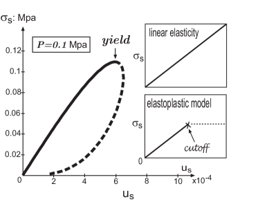
Figure 1: Shear stress versus shear strain for given pressure: for granular elasticity, linear elasticity (upper insert), and elastoplastic theory (lower insert).

Fig. 1 plots σssubscript𝜎𝑠\sigma_{s} versus ussubscript𝑢𝑠u_{s} for the fixed pressure of P=0.1𝑃0.1P=0.1 Mpa. Note how remarkably linear the plot is – almost until yield, where the curve turns back abruptly. (Dashed lines are used throughout for unstable states.) This behavior is approximated by the elastoplastic model, frequently used in soil mechanics: Linear elasticity followed by yield and flat plastic motion, see the lower inserts in Fig. 1. Nonlinearity is relevant only when yield is close.
Refer to caption
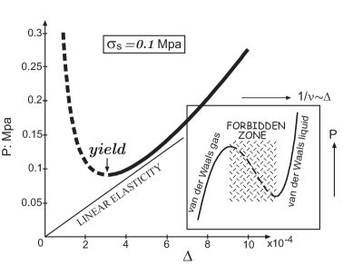
Figure 2: Thick line: Pressure versus compression at fixed shear. Dashed lines represent unstable states. Thin straight line: The same curve for linear elasticity. Insert: The analogous instability in the isothermal curve of the van der Waals equation of state.

If instead ussubscript𝑢𝑠u_{s} is eliminated from Eqs(59,60), the expression

σs2+8𝒜Δ38𝒜PΔ3/2=0superscriptsubscript𝜎𝑠28𝒜superscriptΔ38𝒜𝑃superscriptΔ320\sigma_{s}^{2}+8{\cal AB}\Delta^{3}-8{\cal A}P\Delta^{3/2}=0 (62)

allows a plot of pressure P𝑃P versus compression ΔΔ\Delta, at given σs=0.1subscript𝜎𝑠0.1\sigma_{s}=0.1 Mpa, see Fig. 2. The pressure increases with the compression, implying a positive compressibility, only in the region of large ΔΔ\Delta. The compressibility is negative where ΔΔ\Delta is small, and the stability condition, Eq (53) or (58), is violated. The van der Waals equation of state, (Pa/v2)(vb)=RT𝑃𝑎superscript𝑣2𝑣𝑏𝑅𝑇\left(P-a/v^{2}\right)(v-b)=RT, is quite similar, where 1/v1𝑣1/v corresponds to ΔΔ\Delta, R𝑅R is the gas constant and v𝑣v the molar volume, see eg. Callen . The system can be either in the dense liquid state or the rarefied gaseous phase, with the zone in between forbidden, see insert of Fig. 2.
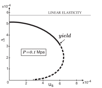
Refer to caption
Figure 3: Compression ΔΔ\Delta versus shear strain ussubscript𝑢𝑠u_{s}, at fixed pressure. The dashed line is again unstable. In linear elasticity, the same curve is a horizontal straight line.
Refer to caption
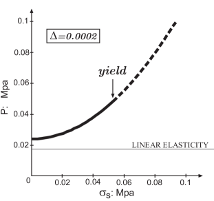
Figure 4: Pressure P𝑃P versus shear stress σssubscript𝜎𝑠\sigma_{s}, at fixed compression. The dashed line is unstable. In linear elasticity, the same curve is a horizontal straight line.

Alternatively, we may plot ΔΔ\Delta versus ussubscript𝑢𝑠u_{s} at fixed P𝑃P, or P𝑃P versus σssubscript𝜎𝑠\sigma_{s} at fixed ΔΔ\Delta, see Figs. 3 and 4, both showing clear evidence of “volume dilatancy,” the fact (first noticed by Reynold) that granular systems expand with shear, or Δ/us|P0evaluated-atΔsubscript𝑢𝑠𝑃0\partial\Delta/\partial u_{s}|_{P}\not=0, or P/σs|Δ0evaluated-at𝑃subscript𝜎𝑠Δ0\partial P/\partial\sigma_{s}|_{\Delta}\not=0. For linear elasticity, these plots are simply horizontal, and the derivatives vanish. If the Boussinesq model, Eq (50), were employed, all four plots would be indistinguishable from those of linear elasticity. So the last term of Eq (52) is indeed essential. (Plastic motion, not considered here, contribute to additional dilatancy, and may dominate.)

III.3 Shear-Dependence of the Elastic Moduli

The Hooke’s law, Eq (46), σij=KΔδij2μuij0subscript𝜎𝑖𝑗𝐾Δsubscript𝛿𝑖𝑗2𝜇superscriptsubscript𝑢𝑖𝑗0\sigma_{ij}=K\Delta\delta_{ij}-2\mu u_{ij}^{0}, may be written as

uij=νEσnnδijσij2μ,subscript𝑢𝑖𝑗𝜈𝐸subscript𝜎𝑛𝑛subscript𝛿𝑖𝑗subscript𝜎𝑖𝑗2𝜇u_{ij}=\frac{\nu}{E}\sigma_{nn}\delta_{ij}-\frac{\sigma_{ij}}{2\mu}, (63)

with the Poisson ratio ν𝜈\nu and the Young modulus E𝐸E given as

E=9μK3K+μ,ν=3K2μ6K+2μ.formulae-sequence𝐸9𝜇𝐾3𝐾𝜇𝜈3𝐾2𝜇6𝐾2𝜇E=\frac{9\mu K}{3K+\mu},\quad\nu=\frac{3K-2\mu}{6K+2\mu}. (64)

Requiring the granular stress-strain relation Eq (52) to assume these familiar forms, either Eq (46) or (63), leads to strain-dependency of K,μ𝐾𝜇K,\mu,

K𝐾\displaystyle K =\displaystyle= Δ1/2(+12𝒜us2/Δ2),superscriptΔ1212𝒜superscriptsubscript𝑢𝑠2superscriptΔ2\displaystyle\Delta^{1/2}\left({\cal B}+\textstyle{\frac{1}{2}}{\cal A}u_{s}^{2}/\Delta^{2}\right), (65)
μ𝜇\displaystyle\mu =\displaystyle= 𝒜Δ1/2,𝒜superscriptΔ12\displaystyle{\cal A}\Delta^{1/2}, (66)

and via Eq (64) also of E,ν𝐸𝜈E,\nu. As this is an intuitive way to characterize nonlinear elastic behavior, we shall consider their shear and pressure dependency more closely here. Using Eqs (59,60), we write these moduli as

μ𝜇\displaystyle\mu =\displaystyle= μ~ξ1/3,K=K~ξ2/3,~𝜇superscript𝜉13𝐾~𝐾superscript𝜉23\displaystyle\widetilde{\mu}\xi^{1/3},\ \ \ \ \ \ \ \ K=\widetilde{K}\xi^{-2/3},
E𝐸\displaystyle E =\displaystyle= E~3+𝒜3+𝒜ξξ13,ν=32𝒜ξ6+2𝒜ξ;~𝐸3𝒜3𝒜𝜉superscript𝜉13𝜈32𝒜𝜉62𝒜𝜉\displaystyle\widetilde{E}\frac{3{\cal B}+{\cal A}}{3{\cal B}+{\cal A}\xi}\xi^{\frac{1}{3}},\ \ \nu=\frac{3{\cal B}-2{\cal A}\xi}{6{\cal B}+2{\cal A}\xi}; (67)

where ξ𝜉\xi quantifies shear,

ξ=12[1±1(/2𝒜)(σs/P)2],𝜉12delimited-[]plus-or-minus112𝒜superscriptsubscript𝜎𝑠𝑃2\xi=\textstyle\frac{1}{2}\left[1\pm\sqrt{1-\left({\cal B}/2{\cal A}\right)\left(\sigma_{s}/P\right)^{2}}\right],\qquad\qquad (68)

and μ~~𝜇\widetilde{\mu}, K~~𝐾\widetilde{K}, E~~𝐸\widetilde{E}, ν~~𝜈\widetilde{\nu} denote the respective value without shear, at ξ=1𝜉1\xi=1,

μ~=𝒜(P)13,K~=(P)13,E~=9𝒜3+𝒜(P)13,formulae-sequence~𝜇𝒜superscript𝑃13formulae-sequence~𝐾superscript𝑃13~𝐸9𝒜3𝒜superscript𝑃13\widetilde{\mu}={\cal A}\left(\frac{P}{\cal B}\right)^{\frac{1}{3}},\ \ \widetilde{K}={\cal B}\left(\frac{P}{\cal B}\right)^{\frac{1}{3}},\ \ \widetilde{E}=\frac{9{\cal AB}}{3{\cal B}+{\cal A}}\left(\frac{P}{\cal B}\right)^{\frac{1}{3}}, (69)

see Fig. 5. (The positive sign in Eq (68) is the stable branch, which meets the unstable branch with the negative sign at yield, where the square root vanishes.)
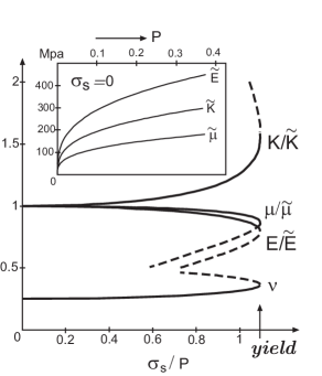
Refer to caption
Figure 5: Variations of K,μ,E,ν𝐾𝜇𝐸𝜈K,\mu,E,\nu with σs/Psubscript𝜎𝑠𝑃\sigma_{s}/P. The moduli are rescaled by their values at σs=0subscript𝜎𝑠0\sigma_{s}=0, denoted respectively with a twiddle. Their variation P1/3similar-toabsentsuperscript𝑃13\sim P^{1/3} is shown in the insert.

As mentioned in the introduction, the P1/3superscript𝑃13P^{1/3}-dependence of the twiddled letters is well-known. For typical granular behavior, however, the more relevant dependence is that on shear, which derives – same as yield and dilatancy – from the last term of Eq (52).

III.4 The Compliance Tensor

III.4.1 Theoretical Expressions

Starting from Eq (52), the tensor Mijksubscript𝑀𝑖𝑗𝑘M_{ijk\ell} of Eq (48) is calculated as

Mijkl=𝒜Δ[(us2/4Δ2+4/33/2𝒜)δijδkl\displaystyle M_{ijkl}={\cal A}\sqrt{\Delta}\,[({u_{s}^{2}}/{4\Delta^{2}}+4/3-{3{\cal B}}/{2{\cal A}})\delta_{ij}\delta_{kl}
δikδjlδilδjk+(uijδkl+δijukl)/Δ].\displaystyle-\delta_{ik}\delta_{jl}-\delta_{il}\delta_{jk}+(u_{ij}\delta_{kl}+\delta_{ij}u_{kl})/\Delta]. (70)

The compliance tensor λijksubscript𝜆𝑖𝑗𝑘\lambda_{ijk\ell}, defined via

duij=λijkdσk,dsubscript𝑢𝑖𝑗subscript𝜆𝑖𝑗𝑘dsubscript𝜎𝑘\text{d}u_{ij}=\lambda_{ijk\ell}\text{d}\sigma_{k\ell}, (71)

is obtained by inverting Mijksubscript𝑀𝑖𝑗𝑘M_{ijk\ell},

λijksubscript𝜆𝑖𝑗𝑘\displaystyle\lambda_{ijk\ell} =\displaystyle= [𝒜us2+2(𝒜)Δ2]δkδij6𝒜Δ1/2(𝒜us22Δ2)δikδj+δiδjk4𝒜Δ1/2delimited-[]𝒜superscriptsubscript𝑢𝑠22𝒜superscriptΔ2subscript𝛿𝑘subscript𝛿𝑖𝑗6𝒜superscriptΔ12𝒜superscriptsubscript𝑢𝑠22superscriptΔ2subscript𝛿𝑖𝑘subscript𝛿𝑗subscript𝛿𝑖subscript𝛿𝑗𝑘4𝒜superscriptΔ12\displaystyle\frac{\left[{\cal A}u_{s}^{2}+2\left({\cal A}-{\cal B}\right)\Delta^{2}\right]\delta_{k\ell}\delta_{ij}}{6{\cal A}\Delta^{1/2}\left({\cal A}u_{s}^{2}-2{\cal B}\Delta^{2}\right)}-\frac{\delta_{ik}\delta_{j\ell}+\delta_{i\ell}\delta_{jk}}{4{\cal A}\Delta^{1/2}} (73)
+uijΔδk+ukΔδij+uijuk3Δ1/2(𝒜us22Δ2),subscript𝑢𝑖𝑗Δsubscript𝛿𝑘subscript𝑢𝑘Δsubscript𝛿𝑖𝑗subscript𝑢𝑖𝑗subscript𝑢𝑘3superscriptΔ12𝒜superscriptsubscript𝑢𝑠22superscriptΔ2\displaystyle+\frac{u_{ij}\Delta\delta_{k\ell}+u_{k\ell}\Delta\delta_{ij}+u_{ij}u_{k\ell}}{3\Delta^{1/2}\left({\cal A}u_{s}^{2}-2{\cal B}\Delta^{2}\right)},
=\displaystyle= 9𝒜5σs2+8(4𝒜9)μ654μ(𝒜5σs28μ6)δkδijδikδj+δiδjk4μ9superscript𝒜5superscriptsubscript𝜎𝑠284𝒜9superscript𝜇654𝜇superscript𝒜5superscriptsubscript𝜎𝑠28superscript𝜇6subscript𝛿𝑘subscript𝛿𝑖𝑗subscript𝛿𝑖𝑘subscript𝛿𝑗subscript𝛿𝑖subscript𝛿𝑗𝑘4𝜇\displaystyle\frac{9{\cal A}^{5}\sigma_{s}^{2}+8\left(4{\cal A}-9{\cal B}\right)\mu^{6}}{54\mu\left({\cal A}^{5}\sigma_{s}^{2}-8\mu^{6}{\cal B}\right)}\delta_{k\ell}\delta_{ij}-\frac{\delta_{ik}\delta_{j\ell}+\delta_{i\ell}\delta_{jk}}{4\mu}
4𝒜3μ3(σij0δk+σk0δij)3𝒜5σij0σk09μ(𝒜5σs28μ6).4superscript𝒜3superscript𝜇3superscriptsubscript𝜎𝑖𝑗0subscript𝛿𝑘superscriptsubscript𝜎𝑘0subscript𝛿𝑖𝑗3superscript𝒜5superscriptsubscript𝜎𝑖𝑗0superscriptsubscript𝜎𝑘09𝜇superscript𝒜5superscriptsubscript𝜎𝑠28superscript𝜇6\displaystyle-\frac{4{\cal A}^{3}\mu^{3}\left(\sigma_{ij}^{0}\delta_{k\ell}+\sigma_{k\ell}^{0}\delta_{ij}\right)-3{\cal A}^{5}\sigma_{ij}^{0}\sigma_{k\ell}^{0}}{9\mu\left({\cal A}^{5}\sigma_{s}^{2}-8\mu^{6}{\cal B}\right)}.

In the first expression λijksubscript𝜆𝑖𝑗𝑘\lambda_{ijk\ell} is strain-, in the second stress-dependent — where the conversion is calculated using Δ=μ2/𝒜2Δsuperscript𝜇2superscript𝒜2\Delta=\mu^{2}/{\cal A}^{2}, uij0=12σij0/μsuperscriptsubscript𝑢𝑖𝑗012superscriptsubscript𝜎𝑖𝑗0𝜇u_{ij}^{0}=-\frac{1}{2}\sigma_{ij}^{0}/\mu, us=12σs/μsubscript𝑢𝑠12subscript𝜎𝑠𝜇u_{s}=\frac{1}{2}\sigma_{s}/\mu, with μ=𝒜(ξP/)1/3𝜇𝒜superscript𝜉𝑃13\mu={\cal A}(\xi P/{\cal B})^{1/3}, cf. Eqs (67,69). The second expression – a surprisingly complicated one if the starting expression for the energy serves as a benchmark – is what may be compared to experiments directly.

Before we do this, it is useful to pause and notice that the last term of both Eq (70) and (73) deviates structurally from the isotropic form of Eq (49). More generally, for an isotropic medium and in the presence of pure compression (σij0=0,P0formulae-sequencesubscriptsuperscript𝜎0𝑖𝑗0𝑃0\sigma^{0}_{ij}=0,\,P\not=0), we may (quite independent of the specific form of the elastic energy) take λijksubscript𝜆𝑖𝑗𝑘\lambda_{ijk\ell} to be

λijk0=λ1δijδk+λ2(δikδj+δiδjk),subscriptsuperscript𝜆0𝑖𝑗𝑘subscript𝜆1subscript𝛿𝑖𝑗subscript𝛿𝑘subscript𝜆2subscript𝛿𝑖𝑘subscript𝛿𝑗subscript𝛿𝑖subscript𝛿𝑗𝑘\lambda^{0}_{ijk\ell}=\lambda_{1}\delta_{ij}\delta_{k\ell}+\lambda_{2}(\delta_{ik}\delta_{j\ell}+\delta_{i\ell}\delta_{jk}), (74)

with λ1,λ2subscript𝜆1subscript𝜆2\lambda_{1},\lambda_{2} arbitrary scalar functions of Δ,usΔsubscript𝑢𝑠\Delta,u_{s}, and the Lode parameter L𝐿L. This is because • both σijsubscript𝜎𝑖𝑗\sigma_{ij} and uksubscript𝑢𝑘u_{k\ell} are symmetric, hence λijk=λjik=λijksubscript𝜆𝑖𝑗𝑘subscript𝜆𝑗𝑖𝑘subscript𝜆𝑖𝑗𝑘\lambda_{ijk\ell}=\lambda_{jik\ell}=\lambda_{ij\ell k}; • the Maxwell relation holds, 2w/uijulk=2w/ulkuijsuperscript2𝑤subscript𝑢𝑖𝑗subscript𝑢𝑙𝑘superscript2𝑤subscript𝑢𝑙𝑘subscript𝑢𝑖𝑗\partial^{2}w/\partial u_{ij}\partial u_{lk}=\partial^{2}w/\partial u_{lk}\partial u_{ij}, hence λijk=λkijsubscript𝜆𝑖𝑗𝑘subscript𝜆𝑘𝑖𝑗\lambda_{ijk\ell}=\lambda_{k\ell ij}. In the presence of shear, σij00subscriptsuperscript𝜎0𝑖𝑗0\sigma^{0}_{ij}\not=0, λijksubscript𝜆𝑖𝑗𝑘\lambda_{ijk\ell} can take on many more terms. To linear order in σij0subscriptsuperscript𝜎0𝑖𝑗\sigma^{0}_{ij}, these are

λ3(σij0δk+δijσk0)+λ4(σik0δj+σi0δjk+σj0δik+σjk0δi).subscript𝜆3subscriptsuperscript𝜎0𝑖𝑗subscript𝛿𝑘subscript𝛿𝑖𝑗subscriptsuperscript𝜎0𝑘subscript𝜆4subscriptsuperscript𝜎0𝑖𝑘subscript𝛿𝑗subscriptsuperscript𝜎0𝑖subscript𝛿𝑗𝑘subscriptsuperscript𝜎0𝑗subscript𝛿𝑖𝑘subscriptsuperscript𝜎0𝑗𝑘subscript𝛿𝑖\lambda_{3}(\sigma^{0}_{ij}\delta_{k\ell}+\delta_{ij}\sigma^{0}_{k\ell})+\lambda_{4}(\sigma^{0}_{ik}\delta_{j\ell}+\sigma^{0}_{i\ell}\delta_{jk}+\sigma^{0}_{j\ell}\delta_{ik}+\sigma^{0}_{jk}\delta_{i\ell}).

To second order, we may substitute all above σij0subscriptsuperscript𝜎0𝑖𝑗\sigma^{0}_{ij} with σik0σkj0subscriptsuperscript𝜎0𝑖𝑘subscriptsuperscript𝜎0𝑘𝑗\sigma^{0}_{ik}\sigma^{0}_{kj}, and also add the terms: σij0σk0subscriptsuperscript𝜎0𝑖𝑗subscriptsuperscript𝜎0𝑘\sigma^{0}_{ij}\sigma^{0}_{k\ell} and σik0σj0+σjk0σi0subscriptsuperscript𝜎0𝑖𝑘subscriptsuperscript𝜎0𝑗subscriptsuperscript𝜎0𝑗𝑘subscriptsuperscript𝜎0𝑖\sigma^{0}_{ik}\sigma^{0}_{j\ell}+\sigma^{0}_{jk}\sigma^{0}_{i\ell}. We shall refer to λijk0subscriptsuperscript𝜆0𝑖𝑗𝑘\lambda^{0}_{ijk\ell} as being isotropic, and the σij0subscriptsuperscript𝜎0𝑖𝑗\sigma^{0}_{ij}-dependent ones as displaying “shear-induced anisotropy.” If the medium were inherently anisotropic, say because the grains are pressed into some quasi-periodic array, leading to a preferred direction 𝐧𝐧\bf{n}, the above expression is more complicated, because δijsubscript𝛿𝑖𝑗\delta_{ij} in Eq (74) may now be substituted by three different tensors: δijninjsubscript𝛿𝑖𝑗subscript𝑛𝑖subscript𝑛𝑗\delta_{ij}-n_{i}n_{j}, ninjsubscript𝑛𝑖subscript𝑛𝑗n_{i}n_{j}, and ϵijknksubscriptitalic-ϵ𝑖𝑗𝑘subscript𝑛𝑘\epsilon_{ijk}n_{k}. For triclinic symmetry and without the Maxwell relation, all 36 elements of λijksubscript𝜆𝑖𝑗𝑘\lambda_{ijk\ell} are independent – even in the absence of shear. As mentioned, this “fabric anisotropy” is not included in the present consideration, because the starting expression for the energy, Eq (51), is isotropic.

III.4.2 Comparison with Experiments

Because σijsubscript𝜎𝑖𝑗\sigma_{ij} and uijsubscript𝑢𝑖𝑗u_{ij} are symmetric, each characterized by six independent components, Eq (71) may be written as a vector equation, du=λ^dσd𝑢^𝜆d𝜎\text{d}\vec{u}=\hat{\lambda}\text{d}\vec{\sigma}, with λ^^𝜆\hat{\lambda} a 6x6 matrix, and du,dσd𝑢d𝜎\text{d}u,\text{d}\sigma given as in Eq (75). In the so-called “principle system” of coordinates, in which σijsubscript𝜎𝑖𝑗\sigma_{ij} is diagonal (but not δσij𝛿subscript𝜎𝑖𝑗\delta\sigma_{ij}), Kuwano and Jardine take this vector equation to be given as Kuwano-Jardine

(du11du22du332du232du132du12)=(000C^000000000G231000000G1310000002G121)(dσ11dσ22dσ33dσ23dσ13dσ12)𝑑subscript𝑢11𝑑subscript𝑢22𝑑subscript𝑢332𝑑subscript𝑢232𝑑subscript𝑢132𝑑subscript𝑢12missing-subexpressionmissing-subexpressionmissing-subexpression000missing-subexpression^𝐶missing-subexpression000missing-subexpressionmissing-subexpressionmissing-subexpression000000superscriptsubscript𝐺231000000superscriptsubscript𝐺1310000002superscriptsubscript𝐺121𝑑subscript𝜎11𝑑subscript𝜎22𝑑subscript𝜎33𝑑subscript𝜎23𝑑subscript𝜎13𝑑subscript𝜎12\left(\begin{array}[]{l}du_{11}\\ du_{22}\\ du_{33}\\ 2du_{23}\\ 2du_{13}\\ 2du_{12}\end{array}\!\!\right)=\left(\begin{array}[]{cccccc}&&&0&0&0\\ &\hat{C}&&0&0&0\\ &&&0&0&0\\ 0&0&0&G_{23}^{-1}&0&0\\ 0&0&0&0&G_{13}^{-1}&0\\ 0&0&0&0&0&2G_{12}^{-1}\end{array}\!\!\right)\!\!\left(\begin{array}[]{l}d\sigma_{11}\\ d\sigma_{22}\\ d\sigma_{33}\\ -d\sigma_{23}\\ -d\sigma_{13}\\ -d\sigma_{12}\end{array}\!\!\right) (75)

with

C^=(1/E1ν12/E2ν13/E3ν21/E11/E2ν23/E3ν31/E1ν32/E21/E3).^𝐶1subscript𝐸1subscript𝜈12subscript𝐸2subscript𝜈13subscript𝐸3subscript𝜈21subscript𝐸11subscript𝐸2subscript𝜈23subscript𝐸3subscript𝜈31subscript𝐸1subscript𝜈32subscript𝐸21subscript𝐸3\displaystyle\hat{C}=\left(\begin{array}[]{ccc}{-1}/{E_{1}}&{\nu_{12}}/{E_{2}}&{\nu_{13}}/{E_{3}}\\ {\nu_{21}}/{E_{1}}&{-1}/{E_{2}}&{\nu_{23}}/{E_{3}}\\ {\nu_{31}}/{E_{1}}&{\nu_{32}}/{E_{2}}&{-1}/{E_{3}}\end{array}\right). (79)

Gijsubscript𝐺𝑖𝑗G_{ij} is referred to as the shear modulus in the ij𝑖𝑗i-j plane, Eisubscript𝐸𝑖E_{i} the Young modulus along i𝑖i, and νijsubscript𝜈𝑖𝑗\nu_{ij} the Poisson ratio for “the effect of the i𝑖i-strain on j𝑗j-strain.” Identifying these moduli with components of the λijksubscript𝜆𝑖𝑗𝑘\lambda_{ijk\ell} tensor,

Gij=1/4λijij,subscript𝐺𝑖𝑗14subscript𝜆𝑖𝑗𝑖𝑗\displaystyle G_{ij}={-1}/{4\lambda_{ijij}},
Ei=1/λiiii,subscript𝐸𝑖1subscript𝜆𝑖𝑖𝑖𝑖\displaystyle E_{i}={-1}/{\lambda_{iiii}},
νij=λiijj/λjjjjsubscript𝜈𝑖𝑗subscript𝜆𝑖𝑖𝑗𝑗subscript𝜆𝑗𝑗𝑗𝑗\displaystyle\nu_{ij}=-{\lambda_{iijj}}/{\lambda_{jjjj}} (80)

(for ij𝑖𝑗i\neq j and without summation over i𝑖i or j𝑗j), we may employ Eq (73) to obtain

G13=G23=G12=μ,subscript𝐺13subscript𝐺23subscript𝐺12𝜇\displaystyle G_{13}=G_{23}=G_{12}=\mu,\qquad\qquad\quad (81)
Ei=27μ(𝒜5σs28μ6)9𝒜5σs272μ6𝒜si2,subscript𝐸𝑖27𝜇superscript𝒜5superscriptsubscript𝜎𝑠28superscript𝜇69superscript𝒜5superscriptsubscript𝜎𝑠272superscript𝜇6𝒜superscriptsubscript𝑠𝑖2\displaystyle E_{i}=\frac{27\mu\left({\cal A}^{5}\sigma_{s}^{2}-8\mu^{6}{\cal B}\right)}{9{\cal A}^{5}\sigma_{s}^{2}-72\mu^{6}{\cal B}-{\cal A}s_{i}^{2}},\qquad (82)
νij=129𝒜5σs272μ6+2𝒜sisj9𝒜5σs272μ6𝒜sj2,subscript𝜈𝑖𝑗129superscript𝒜5superscriptsubscript𝜎𝑠272superscript𝜇62𝒜subscript𝑠𝑖subscript𝑠𝑗9superscript𝒜5superscriptsubscript𝜎𝑠272superscript𝜇6𝒜superscriptsubscript𝑠𝑗2\displaystyle\nu_{ij}=\frac{1}{2}\frac{9{\cal A}^{5}\sigma_{s}^{2}-72\mu^{6}{\cal B}+2{\cal A}s_{i}s_{j}}{9{\cal A}^{5}\sigma_{s}^{2}-72\mu^{6}{\cal B}-{\cal A}s_{j}^{2}}, (83)

with μ=𝒜(ξP/)1/3𝜇𝒜superscript𝜉𝑃13\mu={\cal A}(\xi P/{\cal B})^{1/3}, si3𝒜2σi04μ3subscript𝑠𝑖3superscript𝒜2superscriptsubscript𝜎𝑖04superscript𝜇3s_{i}\equiv 3{\cal A}^{2}\sigma_{i}^{0}-4\mu^{3}, σi0σiPsuperscriptsubscript𝜎𝑖0subscript𝜎𝑖𝑃\sigma_{i}^{0}\equiv\sigma_{i}-P, and σisubscript𝜎𝑖\sigma_{i} denoting the three diagonal components of σijsubscript𝜎𝑖𝑗\sigma_{ij} in the principle system. Before embarking on a comparison, we shall first establish a few qualitative features from theory: • Without shear, σi00superscriptsubscript𝜎𝑖00\sigma_{i}^{0}\rightarrow 0, all Eisubscript𝐸𝑖E_{i} are equal,

EiEsec=27𝒜2𝒜+9(P)13,subscript𝐸𝑖subscript𝐸27𝒜2𝒜9superscript𝑃13E_{i}\rightarrow E_{\sec}=\frac{27{\cal A}{\cal B}}{2{\cal A}+9{\cal B}}\left(\frac{P}{\cal B}\right)^{\frac{1}{3}}, (84)

where Esecsubscript𝐸E_{\sec} is called the secant Young modulus. Same holds for the Poisson ratios,

νijν~=1294𝒜9+2𝒜.subscript𝜈𝑖𝑗superscript~𝜈1294𝒜92𝒜\nu_{ij}\rightarrow\widetilde{\nu}^{*}=\frac{1}{2}\frac{9{\cal B}-4{\cal A}}{9{\cal B}+2{\cal A}}. (85)

(Note ν~superscript~𝜈\widetilde{\nu}^{*} differs from ν~~𝜈\widetilde{\nu}, and Esecsubscript𝐸E_{\sec} from E~~𝐸\widetilde{E}, by a constant factor.) •  Because of Eq (74) and irrespective of the energy specified, we have E1=E2=E3subscript𝐸1subscript𝐸2subscript𝐸3E_{1}=E_{2}=E_{3}, ν12=ν13=ν23subscript𝜈12subscript𝜈13subscript𝜈23\nu_{12}=\nu_{13}=\nu_{23}, and G12=G13=G23subscript𝐺12subscript𝐺13subscript𝐺23G_{12}=G_{13}=G_{23} in the absence of shear, σij0=0subscriptsuperscript𝜎0𝑖𝑗0\sigma^{0}_{ij}=0. Any discrepancy with experiment therefore implies fabric anisotropy. • Finite shear will split Eisubscript𝐸𝑖E_{i} and νijsubscript𝜈𝑖𝑗\nu_{ij}, but not Gijsubscript𝐺𝑖𝑗G_{ij}, cf. Eq (81) — though this is an energy-related feature. • Because of the Maxwell relation, the matrix λ^^𝜆\hat{\lambda} of Eq (75) is symmetric, implying especially (no summation)

νijEi=νjiEj.subscript𝜈𝑖𝑗subscript𝐸𝑖subscript𝜈𝑗𝑖subscript𝐸𝑗\nu_{ij}E_{i}=\nu_{ji}E_{j}. (86)

This symmetry was noted by Love (1927) and adopted by Kuwano and Jardine in interpreting their data Kuwano-Jardine . • The moduli E,μ,ν𝐸𝜇𝜈E,\mu,\nu are related as E=2μ(ν+1)𝐸2𝜇𝜈1E=2\mu\left(\nu+1\right), see Eqs.(64). A similar relation holds for μ𝜇\mu, Eisubscript𝐸𝑖E_{i}, νiksubscript𝜈𝑖𝑘\nu_{ik} [no summation, see Eqs (82,83)],

Ei(6μνijEj)2=4Ej(3μEi)(3μEj)subscript𝐸𝑖superscript6𝜇subscript𝜈𝑖𝑗subscript𝐸𝑗24subscript𝐸𝑗3𝜇subscript𝐸𝑖3𝜇subscript𝐸𝑗E_{i}\left(6\mu\nu_{ij}-E_{j}\right)^{2}=4E_{j}\left(3\mu-E_{i}\right)\left(3\mu-E_{j}\right) (87)
Refer to caption
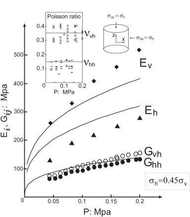
Figure 6: Variation with pressure P𝑃P of the shear moduli Gvh,Ghhsubscript𝐺𝑣subscript𝐺G_{vh},G_{hh}, Young moduli Ev,Ehsubscript𝐸𝑣subscript𝐸E_{v},E_{h} and Poisson ratios νvhsubscript𝜈𝑣\nu_{vh}, νhhsubscript𝜈\nu_{hh} (insert), at σh/σv=0.45subscript𝜎subscript𝜎𝑣0.45\sigma_{h}/\sigma_{v}=0.45. Symbols are the same data on Ham River sand, at a void ratio of 0.66 by Kuwano & Jardine, (2002).

It is important to realize that all formulas of this section hold not only for Cartesian coordinates, ix,y,z𝑖𝑥𝑦𝑧i\to x,y,z, but also for cylindrical ones, iz,ρ,φ𝑖𝑧𝜌𝜑i\to z,\rho,\varphi. Taking Δ=uφφ+uρρ+uzzΔsubscript𝑢𝜑𝜑subscript𝑢𝜌𝜌subscript𝑢𝑧𝑧\Delta=u_{\varphi\varphi}+u_{\rho\rho}+u_{zz}, and similarly for ussubscript𝑢𝑠u_{s}, we may again start from the same energy, Eq (51), and derive all the results here. [Spatial differentiation is what mars the similarity. Yet once the strain components uρρ,uρφsubscript𝑢𝜌𝜌subscript𝑢𝜌𝜑u_{\rho\rho},u_{\rho\varphi}\dots are given, no spatial differentiation is needed.] The one difference is, for any constant σijsubscript𝜎𝑖𝑗\sigma_{ij} in Cartesian coordinates, there is always a principle system. In cylindrical coordinates, this holds only if the stress is also cylindrically symmetric. In other words, only if the stress is uniaxially diagonal, σij=diag(σ1,σ2,σ3)subscript𝜎𝑖𝑗diagsubscript𝜎1subscript𝜎2subscript𝜎3\sigma_{ij}=\text{diag}(\sigma_{1},\sigma_{2},\sigma_{3}) with σ2=σ1subscript𝜎2subscript𝜎1\sigma_{2}=\sigma_{1} in Cartesian coordinates, will it be diagonal cylindrically.

Because Kuwano and Jardine Kuwano-Jardine used an axialsymmetric device for their measurements, the stress they apply is indeed cylindrically symmetric, with: Gρz=Gφzsubscript𝐺𝜌𝑧subscript𝐺𝜑𝑧G_{\rho z}=G_{\varphi z}, Eρ=Eφsubscript𝐸𝜌subscript𝐸𝜑E_{\rho}=E_{\varphi}, νρz=νφzsubscript𝜈𝜌𝑧subscript𝜈𝜑𝑧\nu_{\rho z}=\nu_{\varphi z}, νzρ=νzφsubscript𝜈𝑧𝜌subscript𝜈𝑧𝜑\nu_{z\rho}=\nu_{z\varphi}, cf. Eqs.(81-83) noting sρ=sφsubscript𝑠𝜌subscript𝑠𝜑s_{\rho}=s_{\varphi}. In addition, Eq (86) leads to νρφ=νφρsubscript𝜈𝜌𝜑subscript𝜈𝜑𝜌\nu_{\rho\varphi}=\nu_{\varphi\rho}. Following them, we refer to the response coefficients being measured as: GhhGρφsubscript𝐺subscript𝐺𝜌𝜑G_{hh}\equiv G_{\rho\varphi}, GvhGρz=Gφzsubscript𝐺𝑣subscript𝐺𝜌𝑧subscript𝐺𝜑𝑧G_{vh}\equiv G_{\rho z}=G_{\varphi z}, EhEρ=Eφsubscript𝐸subscript𝐸𝜌subscript𝐸𝜑E_{h}\equiv E_{\rho}=E_{\varphi}, EvEzsubscript𝐸𝑣subscript𝐸𝑧E_{v}\equiv E_{z}, νhhνρφ=νφρsubscript𝜈subscript𝜈𝜌𝜑subscript𝜈𝜑𝜌\nu_{hh}\equiv\nu_{\rho\varphi}=\nu_{\varphi\rho}, νhvνρz=νφzsubscript𝜈𝑣subscript𝜈𝜌𝑧subscript𝜈𝜑𝑧\nu_{hv}\equiv\nu_{\rho z}=\nu_{\varphi z}, νvhνzρ=νzφsubscript𝜈𝑣subscript𝜈𝑧𝜌subscript𝜈𝑧𝜑\nu_{vh}\equiv\nu_{z\rho}=\nu_{z\varphi}, where hh is the horizontal directions, either ρ𝜌\rho or φ𝜑\varphi, and v𝑣v the vertical direction z𝑧z, see the cylinder of Fig. 6. The main plots of Fig. 6 compare the theoretical curve [calculated by taking σρ=σφ=σhsubscript𝜎𝜌subscript𝜎𝜑subscript𝜎\sigma_{\rho}=\sigma_{\varphi}=\sigma_{h} and σz=σvsubscript𝜎𝑧subscript𝜎𝑣\sigma_{z}=\sigma_{v} in Eqs.(81-83)] and the experimental data [measured with Ham River sand] of Ehsubscript𝐸E_{h}, Evsubscript𝐸𝑣E_{v}, Gvhsubscript𝐺𝑣G_{vh}, Ghhsubscript𝐺G_{hh}, as functions of P𝑃P, for σh=0.45σvsubscript𝜎0.45subscript𝜎𝑣\sigma_{h}=0.45\,\sigma_{v}. The insert shows the same comparison for νvh,νhhsubscript𝜈𝑣subscript𝜈\nu_{vh},\nu_{hh}. We especially note that theory and experiment agree on the ordering of the induced anisotropy, ie νvh>νhhsubscript𝜈𝑣subscript𝜈\nu_{vh}>\nu_{hh}, Ev>Ehsubscript𝐸𝑣subscript𝐸E_{v}>E_{h} and GhhGvhsubscript𝐺subscript𝐺𝑣G_{hh}\approx G_{vh}, which are pairwise equal in linear elasticity and the Boussinesq model. (The slight difference between Ghhsubscript𝐺G_{hh}, Gvhsubscript𝐺𝑣G_{vh} is, as mentioned, the result of fabric anisotropy present in the sample.) For a theory without any useful fit parameter, the agreement must be considered a convincing verification of the elastic approach which, instead of postulating the stress-dependence of 21 (or even 36) independent components of λijklsubscript𝜆𝑖𝑗𝑘𝑙\lambda_{ijkl} directly, looks for one appropriate scalar expression for the energy w𝑤w. Even if it is heavy-handedly simplified, a large number of geometric correlation is preserved by the mere fact that λijklsubscript𝜆𝑖𝑗𝑘𝑙\lambda_{ijkl} is obtained via a double differentiation. This must be the main reason why the calculated λijklsubscript𝜆𝑖𝑗𝑘𝑙\lambda_{ijkl} stands up so surprisingly well when compared to the extensive data of Kuwano-Jardine .
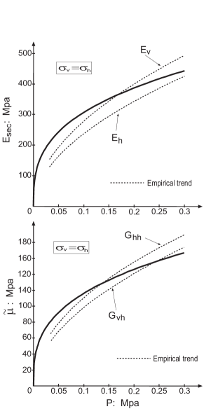
Refer to caption
Figure 7: Variation of Young and shear moduli, Esecsubscript𝐸𝑠𝑒𝑐E_{sec} and μ𝜇\mu, with pressure P𝑃P, for the case of vanishing shear, σv=σhsubscript𝜎𝑣subscript𝜎\sigma_{v}=\sigma_{h}. The dotted lines are the empirical formula of Kuwano & Jardine (2002), for the Ham River sand at the void ratio e=0.66𝑒0.66e=0.66. The split is proof of fabric anisotropy.

Kuwano and Jardine Kuwano-Jardine employ the following empirical formulas (in Mpa) for the Ham River sand,

Evsubscript𝐸𝑣\displaystyle E_{v} =\displaystyle= 204f(σv/Pa)0.52204𝑓superscriptsubscript𝜎𝑣subscript𝑃𝑎0.52\displaystyle 204f\left(\sigma_{v}/P_{a}\right)^{0.52} (88)
Ehsubscript𝐸\displaystyle E_{h} =\displaystyle= 174f(σh/Pa)0.53174𝑓superscriptsubscript𝜎subscript𝑃𝑎0.53\displaystyle 174f\left(\sigma_{h}/P_{a}\right)^{0.53} (89)
Gvhsubscript𝐺𝑣\displaystyle G_{vh} =\displaystyle= 72f(σv/Pa)0.32(σh/Pa)0.272𝑓superscriptsubscript𝜎𝑣subscript𝑃𝑎0.32superscriptsubscript𝜎subscript𝑃𝑎0.2\displaystyle 72f\left(\sigma_{v}/P_{a}\right)^{0.32}\left(\sigma_{h}/P_{a}\right)^{0.2} (90)
Ghhsubscript𝐺\displaystyle G_{hh} =\displaystyle= 81f(σv/Pa)0.04(σh/Pa)0.5381𝑓superscriptsubscript𝜎𝑣subscript𝑃𝑎0.04superscriptsubscript𝜎subscript𝑃𝑎0.53\displaystyle 81f\left(\sigma_{v}/P_{a}\right)^{-0.04}\left(\sigma_{h}/P_{a}\right)^{0.53} (91)

where Pa=0.1013subscript𝑃𝑎0.1013P_{a}=0.1013 Mpa is the atmospheric pressure and f=(2.17e)2/(1+e)𝑓superscript2.17𝑒21𝑒f=(2.17-e)^{2}/(1+e). (f=1.3736𝑓1.3736f=1.3736 for the void ratio e=0.66𝑒0.66e=0.66.) Fig. 7 shows the theoretical and experimental values for Ehsubscript𝐸E_{h}, Evsubscript𝐸𝑣E_{v}, Gvhsubscript𝐺𝑣G_{vh} and Ghhsubscript𝐺G_{hh}, as functions of P𝑃P for the isotropic case σh=σvsubscript𝜎subscript𝜎𝑣\sigma_{h}=\sigma_{v}. The fact that Ehsubscript𝐸E_{h}, Evsubscript𝐸𝑣E_{v} and Gvhsubscript𝐺𝑣G_{vh}, Ghhsubscript𝐺G_{hh} are pairwise different, indicates (as discussed above) fabric anisotropy. Moreover, the theoretical curves are P1/3similar-toabsentsuperscript𝑃13\sim P^{1/3}, yet experimental ones seem to back a larger power: P1/2similar-toabsentsuperscript𝑃12\sim P^{1/2}. As discussed, • this is a known contradiction between Hertz contact and sound data, with possible explanations provided by GoddardGoddard and de Gennes deGennes96 , • and a question of simplicity versus accuracy in the present approach.
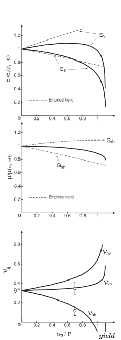
Refer to caption
Figure 8: Upper, middle, and lower figures show the Young moduli, shear moduli and Poisson ratios as functions of σs/Psubscript𝜎𝑠𝑃\sigma_{s}/P. The dotted lines present the empirical formulas of Kuwano & Jardine (2002) for the Ram River sand , at the void ratio e=0.66𝑒0.66e=0.66.

Fig.8 displays the effect of shear on different moduli, with σhσvsubscript𝜎subscript𝜎𝑣\sigma_{h}\not=\sigma_{v}. The upper, middle and lower figures respectively plot the Young moduli Eisubscript𝐸𝑖E_{i}, the shear modulus μ𝜇\mu (both scaled by their isotropic values, Esec,μ~subscript𝐸sec~𝜇E_{\rm sec},\tilde{\mu}), and the Poisson ratios νijsubscript𝜈𝑖𝑗\nu_{ij}. In agreement with the empirical formulas Eqs (88-91), Evsubscript𝐸𝑣E_{v} increases with σs/Psubscript𝜎𝑠𝑃\sigma_{s}/P, while Ehsubscript𝐸E_{h} decreases, in the region away from yield. As yield is approached, both drop quickly to zero. This critical, pre-yield behavior is clearly absent for the empirical formulas and is of interests for future experiments. In theory, Gvh,Ghhsubscript𝐺𝑣subscript𝐺G_{vh},G_{hh} are equal, decreasing with σs/Psubscript𝜎𝑠𝑃\sigma_{s}/P moderately, by less than 20%. In experiments, the shear moduli are split, with one increasing, the other decreasing. The discrepancy between the theory and experiment is in the range from σs/P=0subscript𝜎𝑠𝑃0\sigma_{s}/P=0 to 0.60.60.6 within 20%. This need not be a result from fabric anisotropy, as a more complicated energy expression will also do.

Variation of the Poisson ratios νvh,νhv,νhhsubscript𝜈𝑣subscript𝜈𝑣subscript𝜈\nu_{vh},\nu_{hv},\nu_{hh} is given by Eq (83). As depicted, νvhsubscript𝜈𝑣\nu_{vh} and νhvsubscript𝜈𝑣\nu_{hv} increase, while νhhsubscript𝜈\nu_{hh} decreases, with σs/Psubscript𝜎𝑠𝑃\sigma_{s}/P, all being divergent at yield. No empirical formulae for the ratios are given in Kuwano-Jardine , and the two circles in the plot simply depict the values from the insert of Fig 1. However, νhh=Eh/(2Ghh)1subscript𝜈subscript𝐸2subscript𝐺1\nu_{hh}=E_{h}/(2G_{hh})-1 was assumed to hold by the authors, and interestingly, it may be derived by taking i=h𝑖i=h, j=h𝑗j=h in Eq (87), yielding νhh=Eh/(2μ)1subscript𝜈subscript𝐸2𝜇1\nu_{hh}=E_{h}/(2\mu)-1.

Assuming that both coefficients 𝒜,𝒜\cal A,B of Eq (51) are proportional to f𝑓f of Eqs (88-91), agreement between experiment and theory is extended to all values of the void ratio. Comparison was also made to Kuwano and Jardine’s data gained using glass ballotini Kuwano-Jardine . Taking 𝒜=4200𝒜4200{\cal A}=4200, =53𝒜=700053𝒜7000{\cal B}=\frac{5}{3}{\cal A}=7000, we find similar agreement.

III.5 The Elastic Part of Flow Rules

The increment relation, Eq (48), may also be written in the matrix form dσ=M^dud𝜎^𝑀d𝑢\text{d}\vec{\sigma}=\hat{M}\text{d}\vec{u}, with M^^𝑀\hat{M} a symmetric 6×6666\times 6 matrix, and dσ,dud𝜎d𝑢\text{d}\vec{\sigma},\text{d}\vec{u} still given as in Eq (75). The determinant, detM^=9𝒜5(2Δ2𝒜us2)Δ^𝑀9superscript𝒜52superscriptΔ2𝒜superscriptsubscript𝑢𝑠2Δ\det\hat{M}=9{\cal A}^{5}\left(2{\cal B}\Delta^{2}-{\cal A}u_{s}^{2}\right)\Delta, calculated from Eq (70), vanishes at the yield surface, 𝒜us2=2Δ2𝒜superscriptsubscript𝑢𝑠22superscriptΔ2{\cal A}u_{s}^{2}=2{\cal B}\Delta^{2}, because an Eigenvalue, call it m1subscript𝑚1m_{1}, also does. (This is not a coincidence as M^^𝑀\hat{M} is the Jacobian matrix of the energy function, which is positive only in the stable region. It may be of interest to note that the determinant of the Bousinesq model, detM^=9𝒜5(3+4𝒜)Δ3^𝑀9superscript𝒜534𝒜superscriptΔ3\det\hat{M}=9{\cal A}^{5}\left(3{\cal B}+4{\cal A}\right)\Delta^{3}, never vanishes.) The associated Eigenvector m1subscript𝑚1\vec{m}_{1} points along the direction at which a finite deformation du0d𝑢0\text{d}\vec{u}\neq 0 may take place under constant stress dσij=0dsubscript𝜎𝑖𝑗0\text{d}\sigma_{ij}=0. We refer to m1subscript𝑚1\vec{m}_{1} as the elastic flow direction, since m1duconditionalsubscript𝑚1d𝑢\vec{m}_{1}\|\text{d}\vec{u} is only the elastic contribution of the strain. Setting dσij=0dsubscript𝜎𝑖𝑗0\text{d}\sigma_{ij}=0 in Eq (48) and using 𝒜us2=2Δ2𝒜superscriptsubscript𝑢𝑠22superscriptΔ2{\cal A}u_{s}^{2}=2{\cal B}\Delta^{2}, we obtain

duij=12(δij+uijΔ)dΔ=(2𝒜σij0σsδij3)dΔ.dsubscript𝑢𝑖𝑗12subscript𝛿𝑖𝑗subscript𝑢𝑖𝑗ΔdΔ2𝒜superscriptsubscript𝜎𝑖𝑗0subscript𝜎𝑠subscript𝛿𝑖𝑗3dΔ\text{d}u_{ij}=-\frac{1}{2}\left(\delta_{ij}+\frac{u_{ij}}{\Delta}\right)\text{d}\Delta=\left(\sqrt{\frac{\cal B}{2{\cal A}}}\frac{\sigma_{ij}^{0}}{\sigma_{s}}-\frac{\delta_{ij}}{3}\right)\text{d}\Delta.

The calculated duijdudsubscript𝑢𝑖𝑗d𝑢\text{d}u_{ij}\to\text{d}\vec{u} is the Eigenvector m1subscript𝑚1\vec{m}_{1}. Remarkably, one can rewrite this equation as duij/dΔ=g/σijdsubscript𝑢𝑖𝑗dΔ𝑔subscript𝜎𝑖𝑗\text{d}u_{ij}/\text{d}\Delta=\partial g/\partial\sigma_{ij}, or

m1g/σ,withg=/2𝒜σsP,conditionalsubscript𝑚1𝑔𝜎with𝑔2𝒜subscript𝜎𝑠𝑃\vec{m}_{1}\parallel\partial g/\partial\vec{\sigma},\quad\text{with}\quad g=\sqrt{{\cal B}/2{\cal A}}\sigma_{s}-P, (92)

implying that the elastic flow direction is perpendicular to the yield surface, as defined by the equation g=0𝑔0g=0. If the plastic contribution to the strain field may be neglected for some reasons, this property is referred to as the associated flow rule see wroth ; Huang .

Appendix A energetic stability

In the main text, we considered the convexity of the energy with respect to the variables ussubscript𝑢𝑠u_{s} and ΔΔ\Delta. Relevant is the convexity with respect to uijsubscript𝑢𝑖𝑗u_{ij}. As the transformation between these two sets of variables is nonlinear, we bear the burden of proof that both are equivalent.

Thermodynamic stability requires the elastic energy to be a convex function of its six strain variables, or linear combinations of them. This means that all eigenvalues of the Jacobian matrix 2w/XαXβsuperscript2𝑤subscript𝑋𝛼subscript𝑋𝛽\partial^{2}w/\partial X_{\alpha}\partial X_{\beta} are positive. We take: X1=uxy,X2=uxz,X3=uyzformulae-sequencesubscript𝑋1subscript𝑢𝑥𝑦formulae-sequencesubscript𝑋2subscript𝑢𝑥𝑧subscript𝑋3subscript𝑢𝑦𝑧X_{1}=u_{xy},X_{2}=u_{xz},X_{3}=u_{yz}, X4=(uxxuzz)/2subscript𝑋4subscript𝑢𝑥𝑥subscript𝑢𝑧𝑧2X_{4}=\left(u_{xx}-u_{zz}\right)/2, X5=(uxx2uyy+uzz)/(23)subscript𝑋5subscript𝑢𝑥𝑥2subscript𝑢𝑦𝑦subscript𝑢𝑧𝑧23X_{5}=\left(u_{xx}-2u_{yy}+u_{zz}\right)/(2\sqrt{3}), X6=uxxuyyuzzsubscript𝑋6subscript𝑢𝑥𝑥subscript𝑢𝑦𝑦subscript𝑢𝑧𝑧X_{6}=-u_{xx}-u_{yy}-u_{zz}, with Q=us2=2α=15Xα2𝑄superscriptsubscript𝑢𝑠22superscriptsubscript𝛼15superscriptsubscript𝑋𝛼2Q=u_{s}^{2}=2\sum_{\alpha=1}^{5}X_{\alpha}^{2}. For an energy of the form w=w(Δ,Q)=w(X6,Q)𝑤𝑤Δ𝑄𝑤subscript𝑋6𝑄w=w(\Delta,Q)=w(X_{6},Q) and denoting f4w/Q𝑓4𝑤𝑄f\equiv 4\partial w/\partial Q, a2w/Δ2𝑎superscript2𝑤superscriptΔ2a\equiv\partial^{2}w/\partial\Delta^{2}, b42w/QΔ𝑏4superscript2𝑤𝑄Δb\equiv 4\partial^{2}w/\partial Q\partial\Delta, c=162w/Q2𝑐16superscript2𝑤superscript𝑄2c=16\partial^{2}w/\partial Q^{2}, the Jacobian matrix is

(f+cX12cX1X2cX1X3cX1X4cX1X5bX1cX1X2f+cX22cX2X3cX2X4cX2X5bX2cX1X3cX2X3f+cX32cX3X4cX3X5bX3cX1X4cX2X4cX3X4f+cX42cX4X5bX4cX1X5cX2X5cX3X5cX4X5f+cX52bX5bX1bX2bX3bX4bX5a)𝑓𝑐superscriptsubscript𝑋12𝑐subscript𝑋1subscript𝑋2𝑐subscript𝑋1subscript𝑋3𝑐subscript𝑋1subscript𝑋4𝑐subscript𝑋1subscript𝑋5𝑏subscript𝑋1𝑐subscript𝑋1subscript𝑋2𝑓𝑐superscriptsubscript𝑋22𝑐subscript𝑋2subscript𝑋3𝑐subscript𝑋2subscript𝑋4𝑐subscript𝑋2subscript𝑋5𝑏subscript𝑋2𝑐subscript𝑋1subscript𝑋3𝑐subscript𝑋2subscript𝑋3𝑓𝑐superscriptsubscript𝑋32𝑐subscript𝑋3subscript𝑋4𝑐subscript𝑋3subscript𝑋5𝑏subscript𝑋3𝑐subscript𝑋1subscript𝑋4𝑐subscript𝑋2subscript𝑋4𝑐subscript𝑋3subscript𝑋4𝑓𝑐superscriptsubscript𝑋42𝑐subscript𝑋4subscript𝑋5𝑏subscript𝑋4𝑐subscript𝑋1subscript𝑋5𝑐subscript𝑋2subscript𝑋5𝑐subscript𝑋3subscript𝑋5𝑐subscript𝑋4subscript𝑋5𝑓𝑐superscriptsubscript𝑋52𝑏subscript𝑋5𝑏subscript𝑋1𝑏subscript𝑋2𝑏subscript𝑋3𝑏subscript𝑋4𝑏subscript𝑋5𝑎\left(\begin{array}[]{llllll}f+cX_{1}^{2}&cX_{1}X_{2}&cX_{1}X_{3}&cX_{1}X_{4}&cX_{1}X_{5}&bX_{1}\\ cX_{1}X_{2}&f+cX_{2}^{2}&cX_{2}X_{3}&cX_{2}X_{4}&cX_{2}X_{5}&bX_{2}\\ cX_{1}X_{3}&cX_{2}X_{3}&f+cX_{3}^{2}&cX_{3}X_{4}&cX_{3}X_{5}&bX_{3}\\ cX_{1}X_{4}&cX_{2}X_{4}&cX_{3}X_{4}&f+cX_{4}^{2}&cX_{4}X_{5}&bX_{4}\\ cX_{1}X_{5}&cX_{2}X_{5}&cX_{3}X_{5}&cX_{4}X_{5}&f+cX_{5}^{2}&bX_{5}\\ bX_{1}&bX_{2}&bX_{3}&bX_{4}&bX_{5}&a\end{array}\!\!\right)

with its six eigenvalues given as f14=fsubscript𝑓14𝑓f_{1-4}=f and

f±=f+a2+cQ4±12(fa+cQ2)2+2b2Q.subscript𝑓plus-or-minusplus-or-minus𝑓𝑎2𝑐𝑄412superscript𝑓𝑎𝑐𝑄222superscript𝑏2𝑄f_{\pm}=\frac{f+a}{2}+\frac{cQ}{4}\pm\frac{1}{2}\sqrt{\left(f-a+\frac{cQ}{2}\right)^{2}+2b^{2}Q}. (93)

They are all positive if, and only if, f>0𝑓0f>0, 2af+acQb2Q>02𝑎𝑓𝑎𝑐𝑄superscript𝑏2𝑄02af+acQ-b^{2}Q>0, f+a+cQ/2>0𝑓𝑎𝑐𝑄20f+a+cQ/2>0, or equivalently,

wQ>0,4wQ+2wΔ2+8Q2wQ2>0.formulae-sequence𝑤𝑄04𝑤𝑄superscript2𝑤superscriptΔ28𝑄superscript2𝑤superscript𝑄20\displaystyle\frac{\partial w}{\partial Q}>0,\qquad 4\frac{\partial w}{\partial Q}+\frac{\partial^{2}w}{\partial\Delta^{2}}+8Q\frac{\partial^{2}w}{\partial Q^{2}}>0. (94)
2wΔ2wQ+2Q2wQ22wΔ22Q(2wQΔ)2>0,superscript2𝑤superscriptΔ2𝑤𝑄2𝑄superscript2𝑤superscript𝑄2superscript2𝑤superscriptΔ22𝑄superscriptsuperscript2𝑤𝑄Δ20\displaystyle\frac{\partial^{2}w}{\partial\Delta^{2}}\frac{\partial w}{\partial Q}+2Q\frac{\partial^{2}w}{\partial Q^{2}}\frac{\partial^{2}w}{\partial\Delta^{2}}-2Q\left(\frac{\partial^{2}w}{\partial Q\partial\Delta}\right)^{2}>0, (95)

Because us2=Qsuperscriptsubscript𝑢𝑠2𝑄u_{s}^{2}=Q, or 2us(w/Q)=w/us2subscript𝑢𝑠𝑤𝑄𝑤subscript𝑢𝑠2u_{s}\left(\partial w/\partial Q\right)=\partial w/\partial u_{s}, 2us(2w/ΔQ)=2w/Δus2subscript𝑢𝑠superscript2𝑤Δ𝑄superscript2𝑤Δsubscript𝑢𝑠2u_{s}\left(\partial^{2}w/\partial\Delta\partial Q\right)=\partial^{2}w/\partial\Delta\partial u_{s}, 4usQ×(2w/Q2)=us(2w/us2)w/us4subscript𝑢𝑠𝑄superscript2𝑤superscript𝑄2subscript𝑢𝑠superscript2𝑤superscriptsubscript𝑢𝑠2𝑤subscript𝑢𝑠4u_{s}Q\times\left(\partial^{2}w/\partial Q^{2}\right)=u_{s}\left(\partial^{2}w/\partial u_{s}^{2}\right)-\partial w/\partial u_{s}, these conditions are equivalent to Eqs (55,56), or

wΔ>0,2wΔ2>0,2wus2>0,formulae-sequence𝑤Δ0formulae-sequencesuperscript2𝑤superscriptΔ20superscript2𝑤superscriptsubscript𝑢𝑠20\displaystyle\frac{\partial w}{\partial\Delta}>0,\ \frac{\partial^{2}w}{\partial\Delta^{2}}>0,\ \frac{\partial^{2}w}{\partial u_{s}^{2}}>0, (96)
2wΔ22wus2>(2wusΔ)2.superscript2𝑤superscriptΔ2superscript2𝑤superscriptsubscript𝑢𝑠2superscriptsuperscript2𝑤subscript𝑢𝑠Δ2\displaystyle\frac{\partial^{2}w}{\partial\Delta^{2}}\frac{\partial^{2}w}{\partial u_{s}^{2}}>\left(\frac{\partial^{2}w}{\partial u_{s}\partial\Delta}\right)^{2}. (97)

For the energy of Eq (51), the inequalities (96) imply 𝒜>0,>0formulae-sequence𝒜00{\cal A}>0,{\cal B}>0, while Eq (97) gives the yield condition (57). Using P=w/Δ𝑃𝑤ΔP=\partial w/\partial\Delta and σs=w/ussubscript𝜎𝑠𝑤subscript𝑢𝑠\sigma_{s}=\partial w/\partial u_{s} we can also write Eqs (96,97) as

(PΔ)us>0,(σsus)Δ>0,formulae-sequencesubscript𝑃Δsubscript𝑢𝑠0subscriptsubscript𝜎𝑠subscript𝑢𝑠Δ0\displaystyle\left(\frac{\partial P}{\partial\Delta}\right)_{u_{s}}>0,\ \ \left(\frac{\partial\sigma_{s}}{\partial u_{s}}\right)_{\Delta}>0, (98)
(PΔ)us(σsus)Δ>(Pus)Δ2subscript𝑃Δsubscript𝑢𝑠subscriptsubscript𝜎𝑠subscript𝑢𝑠Δsuperscriptsubscript𝑃subscript𝑢𝑠Δ2\displaystyle\left(\frac{\partial P}{\partial\Delta}\right)_{u_{s}}\left(\frac{\partial\sigma_{s}}{\partial u_{s}}\right)_{\Delta}>\left(\frac{\partial P}{\partial u_{s}}\right)_{\Delta}^{2} (99)

The Maxwell relation P/us|Δ=σs/Δ|usevaluated-at𝑃subscript𝑢𝑠Δevaluated-atsubscript𝜎𝑠Δsubscript𝑢𝑠\left.\partial P/\partial u_{s}\right|_{\Delta}=\left.\partial\sigma_{s}/\partial\Delta\right|_{u_{s}} and the thermodynamic identities P/Δ|us=P/Δ|σs+P/σs|Δσs/Δ|usevaluated-at𝑃Δsubscript𝑢𝑠evaluated-at𝑃Δsubscript𝜎𝑠evaluated-atevaluated-at𝑃subscript𝜎𝑠Δsubscript𝜎𝑠Δsubscript𝑢𝑠\left.\partial P/\partial\Delta\right|_{u_{s}}=\left.\partial P/\partial\Delta\right|_{\sigma_{s}}+\left.\partial P/\partial\sigma_{s}\right|_{\Delta}\cdot\left.\partial\sigma_{s}/\partial\Delta\right|_{u_{s}}, P/us|Δ=P/σs|Δσs/us|Δevaluated-at𝑃subscript𝑢𝑠Δevaluated-atevaluated-at𝑃subscript𝜎𝑠Δsubscript𝜎𝑠subscript𝑢𝑠Δ\left.\partial P/\partial u_{s}\right|_{\Delta}=\left.\partial P/\partial\sigma_{s}\right|_{\Delta}\cdot\left.\partial\sigma_{s}/\partial u_{s}\right|_{\Delta} , imply an alternative stability condition,

(P/Δ)σs>0.subscript𝑃Δsubscript𝜎𝑠0\left(\partial P/\partial\Delta\right)_{\sigma_{s}}>0. (100)

References

  • (1) Y.M. Jiang, M. Liu, Phys. Rev. Lett., 91, 144301 (2003), 93, 148001(2004); Eur. Phys. J. E., 1292-8941(2007).
  • (2) D.O. Krimer, M. Pfitzner, K. Bräuer, Y. Jiang, M. Liu, Phys. Rev. E74, 061310 (2006); K. Bräuer, M. Pfitzner, D.O. Krimer, M. Mayer, Y. Jiang, M. Liu, Phys. Rev. E74, 061311 (2006); Y.M. Jiang, M. Liu, Eur. Phys. J. E., 1292-8941(2007).
  • (3) P. K. Haff, J. Fluid Mech., 134, 401(1983); J. T. Jenkins and S. B. Savage, J. Fluid Mech., 130, 187(1983).
  • (4) L.E. Silbert, D. Ertas, G.S. Grest, T.C. Halsey, D. Levine, S.J. Plimpton, Phys. Rev. E 64, 051302 (2001); GDR MiDi group, Eur. Phys. J. E 14, 341 (2004); P.Jop, Y. Forterre, O. Pouliquen, Nature 441, 727, 2006.
  • (5) Y.M. Jiang, M. Liu, Cond-Mat, arXiv:0706.1354
  • (6) D. Kolymbas, Introduction to Hypoplasticity, (Balkema, Rotterdam, 2000); W. Wu and D. Kolymbas, in Constitutive Modelling of Granular Materials ed Kolymbas, (Springer, Berlin, 2000), and references therein.
  • (7) H. Temmen, H. Pleiner, M. Liu and H.R. Brand, Phys. Rev. Lett. 84, 3228 (2000) and 86, 745 (2001); H. Pleiner, M. Liu and H.R. Brand, Acta Rheol. 39, 560 (2000)
  • (8) G.H. Helfrich, Phys.Rev.Lett 23, 372 (1969); P.G. de Gennes, J. Prost, The Physics of Liquid Crystals (Clarendon Press, Oxford, 1993); H. Pleiner, H.R. Brand, in Pattern Formation in Liquid Crystals eds. A. Buka, L. Kramer, (Springer, New York, 1996); P.C. Martin, O. Parodi, and P.S. Pershan, Phys. Rev. A 6, 2401 (1972).
  • (9) T. Komatsu, S. Inagaki, N. Nakagawa, and S. Nasuno, Phys. Rev. Lett. 86, 1757 (2001).
  • (10) O. Müller, PhD-thesis, (2006), University Tübingen; O. Müller, M. Liu, H. Pleiner and H.R. Brand, preprint.
  • (11) L. Bocquet, J. Errami, and T. C. Lubensky, Phys. Rev. Lett., 89, 184301 (2002); W. Losert, L. Bocquet, T. C. Lubensky, and J. P. Gollub, Phys. Rev. Lett., 85, 1428 (2000); L. Bocquet, W. Losert, D. Schalk, T. C. Lubensky, and J. P. Gollub, Phys. Rev., E 65, 11307 (2001); I. Goldhirsch, Annu. Reev. Fluid Mech., 35, 267(2003).
  • (12) S.F. Edwards, R.B.S. Oakeshott, Physica A 157, 1080 (1989); A. Metha, S.F. Edwards, Physica A 157, 1091.
  • (13) P. Richard, M. Nicodemi, R. Delannay, P. Ribiere and D. Bideau, Nature Materials, 4, 121(2005).
  • (14) L. D. Landau, and E. M. Lifshitz, Theory of Elasticity (New York, Pergamon Press, 3rd edn. 1986)
  • (15) G. Gudehus, in In Constitutive relations for soils, eds G. Gudehus, F. Darve, and I. Vardoulakis, (Rotterdam, Balkema, 1984).
  • (16) P. Evesque and P. G. de Gennes, C. R. Acad. Sci. Paris, 326, 761 (1998); P. G. de Gennes, Rev. Mod. Phys., 71, 347 (1999).
  • (17) J. D. Goddard, Proc. R. Soc. London, A430, 105 (1990).
  • (18) R. Kuwano, and R. J. Jardine, Géotechnique, 52, 727 (2002).
  • (19) F. Alonso-Marroquin, H.J. Herrmann, Phys. Rev. Lett. 92, 054301 (2004).
  • (20) H. B. Callen, Thermodynamics (New York, John Wiley & Sons, 1960).
  • (21) de Gennes, P. G. Europhys. Lett., 35, 145 (1996).
  • (22) A. Schofield and P. Wroth, Critical state soil state mechanics, (London, Mcgrau-Hill 1968).
  • (23) W. X. Huang, Engineering properties of soil, in Chinese (Beijing, Hydroelectricity publishing, 1983).