Cluster abundances and S-Z power spectra: effects of non-Gaussianity and early dark energy

Abstract

In the standard $\Lambda$CDM cosmological model with a Gaussian primordial density fluctuation field, the relatively low value of the mass variance parameter ($\sigma_{8}=0.74^{+0.05}_{-0.06}$, obtained from the WMAP 3-year data) results in a reduced likelihood that the measured level of CMB anisotropy on the scales of clusters is due to the Sunyaev-Zeldovich (S-Z) effect. To assess the feasibility of producing higher levels of S-Z power, we explore two alternative models which predict higher cluster abundance. In the first model the primordial density field has a $\chi^{2}_{1}$ distribution, whereas in the second an early dark energy component gives rise to the desired higher cluster abundance. We carry out the necessary detailed calculations of the levels of S-Z power spectra, cluster number counts, and angular 2-point correlation function of clusters, and compare (in a self-consistent way) their predicted redshift distributions. Our results provide a sufficient basis upon which the viability of the three models may be tested by future high quality measurements.

1 INTRODUCTION

Measurements with the BIMA (Dawson et al. 2002), CBI (Readhead et al. 2004), and ACBAR (Kuo et al. 2004) experiments indicate a significant power excess at high multipoles ($\ell>5000$ in the former, $\ell\sim 3000$ in the two latter cases) with respect to theoretically predicted levels of the primary CMB anisotropy. It has been suggested that the excess could be due to the S-Z effect, but its observed level would require a rather high value of $\sigma_{8}$ ($\gtrsim 1$) in order to have the necessary large number of massive clusters, with the largest relative contribution to the S-Z power spectrum. Such a high value is usually disfavoured in cluster studies, and is at clear variance with results from the latest WMAP 3-year data, according to which $\sigma_{8}=0.74^{+0.05}_{-0.06}$ (Spergel et al. 2006). If the reported excess is indeed due to the S-Z effect, modifications to the standard $\Lambda$CDM cosmological model may be required in order to account for the implied higher number of clusters.

Cluster abundance at high redshift can be boosted by the presence of a scale-dependent, non-Gaussian, positively skewed component in the primordial density fluctuation field, as was demonstrated by Mathis, Diego, & Silk (2004), and Sadeh, Rephaeli, & Silk (2006) (hereafter SRS). In such a model, primordial overdensities attain larger amplitudes with higher probabilities than the corresponding overdensities in a purely Gaussian random field, and may therefore give rise to earlier cluster formation and to higher numbers of massive clusters. In both works the former WMAP 1-year normalisation was employed ($\sigma_{8}=0.9$), and it was shown that already with this relatively high value it is difficult to reconcile the CMB power excess with the inferred cluster population, if the underlying fluctuation field obeys Gaussian statistics. On the other hand, a $\chi^{2}_{1}$ distributed field was demonstrated to be capable of producing a sufficiently large cluster population, and consequently S-Z power levels that are consistent with the above mentioned observational results. The $\chi^{2}_{m}$ family of models was originally proposed by Peebles (1997, 1999a,b), and is based on an isocurvature cold dark matter (CDM) scenario in which the primordial density field is proportioinal to the square of a random Gaussian process (Peebles 1997). Implications of this model on the primary CMB anisotropy and the dynamics and evolution of the large scale strcuture have been the subject of several studies (e.g. Koyama, Soda & Taruya 1999, Mathis, Diego & Silk 2004). Other theoretically motivated non-Gaussian models found in the literature include, e.g., the log-normal probability distribution function. A rather comprehensive list of such models and their statistical properties are explored in detail in Coles & Barrow (1987). A common parametrization of non-Gaussianity is provided by the following transformation on an underlying Gaussian field:

$$\psi(x)=\alpha\phi(x)+\epsilon\left[\phi^{2}(x)-\langle\phi^{2}\rangle\right].$$ (1)

The parameter $\epsilon$, alternatively written as $f_{NL}$ and referred to as the nonlinear coupling factor, characterises the amplitude of the quadratic term. In this respect, the $\chi^{2}_{m}$ model constitues a special case in which $\alpha=0$. The degree of non-Gaussianity of a given model is defined in several ways; these include the skewness of the density field (for which a one-to-one correspondence with the nonlinear coupling term can be derived; Matarrese, Verde & Jimenez 2000), and the parameter $\zeta$ defined as

$$\zeta(M)=\frac{\int_{3\sigma}^{\infty}p(\delta,M)d\delta}{\int_{3\sigma}^{\infty}p_{G}(\delta,M)d\delta},$$ (2)

which describes the 3-$\sigma$ tail excess probability of the non-Gaussian model over the Gaussian probability distribution function. For the $\chi^{2}_{1}$ model $\zeta=16.3$. While there seems to be observational evidence for a lower level of non-Gaussianity ($\zeta\lesssim 4$, Robinson & Baker 2000; Avila-Reese et al. 2003, and $\zeta\lesssim 1.6$, Robinson, Gawiser, & Silk 2000; Komatsu et al. 2003), we believe that these results do not necessarily rule out models with higher levels of non-Gaussianity. This is due to the fact that these results were inferred either from primary CMB anisotropy observations, which explore scales much larger than those associated with clusters of galaxies, and therefore, lower overdensities, which may be indistinguishable from a non-Gaussian distribution in case the density field is scale-variant, or from observations of low-redshift clusters, whereas - as will be shown below - the non-Gaussian tail would be mainly manifested in an enhanced high-redshift cluster population.

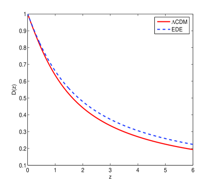
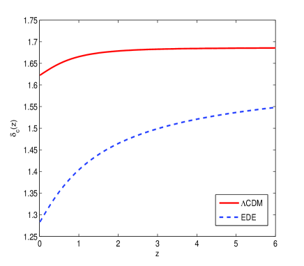
Early dark energy (hereafter EDE) models provide an alternative for generating higher cluster populations at higher redshifts. In these models the dark energy density is appreciable already at early epochs of cosmic evolution, and attains the observationally inferred value at present. Consequently, the quintessence equation of state coefficient changes with time. Such models have been the subject of study by several authors who investigated their potential influence on the CMB (Doran et al. 2001a, Caldwell et al. 2003), and the linear growth of structure (Ferreira & Joyce 1998, Doran et al. 2001b). More recently, Bartelmann, Doran, & Wetterich (2006; hereafter BDW) have carried out a comprehensive study of two specific EDE models, evaluating numerically the quantities relevant to structure formation and the halo mass function, such as the linear growth factor of density perturbations, critical density for spherical collapse, and the overdensity at virialisation. Specifically, they find that with respect to their corresponding values in the standard $\Lambda$CDM model, a slower evolution of the linear growth factor and reduced values of the critical density for spherical collapse are predicted. As noted by BDW, the slower evolution of the linear growth factor in EDE models is a consequence of the higher expansion rate of the universe at early times due to an early acceleration phase caused by the non-vanishing dark energy component. Therefore, with a given value of the present mass variance normalisation the corresponding quantity at early times should be larger than what is implied in the $\Lambda$CDM model. Since the critical overdensity for collapse at a given redshift is the linearly extrapolated value from the early universe, the slower evolution of the growth factor in EDE models is manifested by a lower critical density with respect to the $\Lambda$CDM model at all redshifts relevant to structure formation. Hence, the cluster population, which increases with decreasing $\delta_{c}$ and increasing $\sigma_{M}$, grows considerably.

In this paper we focus on the impact of these two alternative scenarios on S-Z observables, namely the angular power spectrum of CMB temperature variations due to the S-Z effect, and the angular 2-point correlation function (hereafter A2PCF) of clusters. As is demonstrated below, the higher abundance of massive clusters at high redshifts in the non-Gaussian and EDE models boosts S-Z power levels (as a result of higher values of the Comptonization parameter), which in turn gives rise to larger temperature variations in the CMB. Conversely, the A2PCF is demonstrated to predict lower correlation levels in the EDE, and in particular, the non-Gaussian model, owing to the detailed properties of the linear bias parameter, which, with respect to the $\Lambda$CDM model, has a different mass and redshift dependence in the EDE model, and a distinct functional form in the non-Gaussian model.

In §2 we briefly describe the Press & Schechter mass function variant adapted to the $\chi^{2}_{1}$-distributed probability distribution function (PDF) of the primordial density fluctuation field, and outline the properties of the EDE model adopted in our calculations. Results of the calculations are described in §3, where S-Z power levels calculated for the standard $\Lambda$CDM, EDE, and non-Gaussian models are compared with the BIMA, CBI, and ACBAR observational results, and an account of the A2PCF for these 3 models is given. §4 includes a discussion and our conclusions. In the appendix we provide a brief exposition of the differential equations governing the redshift evolution of the comoving radial distance, linear growth factor of density perturbations, critical density for spherical collapse, and overdensity at virialisation corresponding to the EDE model, and present some numerical results.

2 METHOD

The standard $\Lambda$CDM, EDE, and non-Gaussian models will be referred to hereafter as models I, II, and III, respectively. A full account of models I and III is provided in SRS; here we only include new relevant aspects of these two models. We adopt a Press & Schechter (1974) mass function of the form

$$n(M,z)=-\mu F(\mu)\frac{\rho_{b}}{M\sigma_{M}^{2}(z)}\frac{d\sigma}{dM}\,dM,$$ (3)

where $\mu\equiv\delta_{c}(z)/\sigma_{M}(z)$ is the critical overdensity for collapse in terms of the mass variance $\sigma_{M}$ at redshift $z$, and $\rho_{b}$ is the background density at $z=0$. For models I and II,

$$F(\mu)=\sqrt{\frac{2}{\pi}}e^{-(\mu^{2}/2)},$$ (4)

whereas the corresponding expression for model III, for which we take a primordial density fluctuation field obeying $\chi^{2}_{1}$ statistics, is

$$F(\mu)=\frac{e^{-(1+\sqrt{2}\mu)/2}}{\mbox{erfc}[1/\sqrt{2}]\sqrt{\pi(1+\sqrt{2}\mu)}}.$$ (5)

The factor $\mbox{erfc}[1/\sqrt{2}]$ (with erfc representing the complementary error function) in the denominator is introduced in order to arrange that all the mass in the universe be included in haloes, as is similarly accomplished by introducing the well known factor of 2 in the original Press & Schechter mass function. (Recall that the full theoretical justification for this factor is somewhat uncertain; here it is merely introduced to ensure consistency with the mass function of model I). The predicted statistical properties of S-Z observables (i.e. weighted by the cluster population) will be affected by the model of the mass function; clearly, model III differs from models I and II in the functional form of the mass function. Model II differs from both models I and III in the redshift dependence of the critical density for collapse and the linear growth factor of density perturbations, as will be demonstrated below.

For the calculation of the mass variance $\sigma_{R}$ we used a top-hat window function and CDM transfer functions taken from Bardeen et al. (1986): adiabatic transfer function for models I and II, and isocurvature transfer function for model III. Note that the presence of EDE is likely to affect the shape of the CDM transfer function; this effect is minor, however, with a largest difference of $\lesssim 7\%$ at the lowest wave numbers ($k\sim 10^{-4}Mpc^{-1}h$), becoming negligible at higher wave numbers (which correspond to cluster scales), as was verified using the latest version of the CMBFAST code (Zaldarriaga & Seljak 2000), which admits a time-dependent equation of state for dark energy. Consequently, it is reasonable to use the fit provided by Bardeen et al. even in the case of model II.

The calculations were carried out using cosmological parameters deduced from the WMAP 3-year data: $\Omega_{\Lambda}=0.76$ (which, for the case $w\neq-1$ is usually written as $\Omega_{Q}$), $\Omega_{m}=0.24$, $h=0.73$, and $\sigma_{8}=0.74^{+0.05}_{-0.06}$. In addition to these parameters we take the spectral index to be $n=1$ in models I and II, and $n=-1.8$ in model III. Model II requires additional parametrization of the EDE. We use a variant of the EDE models studied in BDW, where we take the density of early quintessence with respect to the critical density to be $\Omega_{e}=.0008$, and the equation of state coefficient at $z=0$ to be $w_{0}=-0.99$. The effective coefficient as a function of redshift is given in the expression (Wetterich 2004)

$$\overline{w}(z)=\frac{w_{0}}{1+u\log{(1+z)}},$$ (6)

where $u\equiv\frac{-3w_{0}}{\log{\left(\frac{1-\Omega_{e}}{\Omega_{e}}\right)}+\log{\left(\frac{1-\Omega_{m}}{\Omega_{m}}\right)}}$.

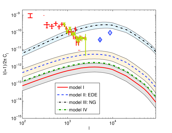
The differential equations governing the evolution of the linear growth factor, critical density for spherical collapse, and overdensity at virialisation pertaining to this model, as well as their numerical solutions, are presented in the Appendix. It is important to note that while our choice of parameters in model I is completely consistent with WMAP results, this is not necessarily the case in models II and III. Nevertheless, we believe that we are able to account for this apparent inconsistency by choosing to normalise the resulting mass functions so as to yield the same (cumulative) cluster density at $z=0$, as predicted by model I. This is justified given the fact that the observables quantified in this study are all related to clusters of galaxies. In fact, it turns out that the same normalisation of $\sigma_{8}=0.74$ (in accordance with WMAP results) induces an identical cumulative cluster density population at $z=0$, as can be clearly seen by inspection Fig. 1. We include for reference a fourth model, which is basically identical to model I, but with a different normalisation of $\sigma_{8}=0.8$. This higher value has been advocated by Evrard et al. (2007), who claim that with a low normalisation, the specific energy in the IC gas and galaxies must increase by $50\%$, which would imply high biases with respect to the cluster dark matter, at variance with what is observed in hydrodynamical simulations. According to Evrard et al., a higher normalisation can solve this conflict, and also provides a better match to recent S-Z observations. These results are actually in line with several cluster studies which seem to indicate higher normalisations than inferred from CMB observations.

The S-Z angular power spectrum was calculated using a formalism similar to that adopted by (e.g.) Cooray (2000), Komatsu & Seljak (2002), and Refregier & Teyssier (2002). Note that these authors have used the NFW formalism to characterise the cluster dark matter profile and the implied IC gas profile. In our calculations we chose to model the IC gas with an isothermal $\beta$-King profile with temperatures derived within the framework of hydrostatic equilibrium. The reason for our selection stems from the fact that the redshift and mass modeling of the concentration parameter appearing in the NFW profile have been carried out on the basis of results from N-body simulations, which usually incorporate primordial Gaussian fields. In such simulations clusters show up only at relatively low redshifts, such that it is not clear whether the deduced fitting of the concentration parameter can really address also higher-redshift clusters, a natural outcome of positively skewed non-Gaussian models. Furthermore, fitting formulae of $c(M,z)$ found in the literature fail to yield meaningful values at redshifts at which clusters may already form in non-Gaussian models. Calculation of the A2PCF of (S-Z) clusters follows the work of SRS and that of Mei & Bartlett (2003); full details can be found in these papers.

3 RESULTS

Figure 1: Cumulative mass functions for models I (continuous), II (dashed), and III (dot-dashed), as a function of cluster mass. The two sets of upper and lower curves correspond to redshifts $z=0.01$ and $z=3$, respectively.

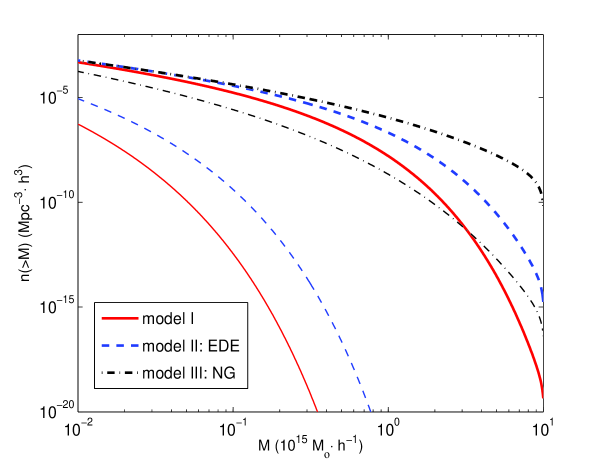
Before we present results of the S-Z power spectrum and A2PCF, it is useful to investigate the behaviour of the mass function in the 3 models at various redshifts. Fig. 1 depicts the cumulative mass function of clusters with masses lying in the range $10^{13}M_{\odot}h^{-1}\leq M\leq 10^{16}M_{\odot}h^{-1}$ at redshifts $z=0.01$ and $z=3$. As can be clearly seen, the three models are correctly normalised so as to yield the same cumulative cluster density at low redshifts. As expected, models II and III consistently predict higher abundances of high-mass clusters than the corresponding high-mass population in the standard $\Lambda$CDM model, with model III dominating over model II. This occurs at both low and high redshifts, and becomes more pronounced with increasing redshift. It appears then that the presence of an excess of high overdensity fluctuations associated with the $\chi^{2}_{1}$ model has a stronger impact on the population of massive clusters than the slower evolution of the linear growth factor and lower values of the critical density for collapse that characterise model II.

The behaviour of the respective mass functions is directly reflected in the S-Z power spectra illustrated in Fig. 2. Here the enhanced massive cluster population, particularly at relatively high redshifts, is manifested in both increased power levels ($\sim 1\cdot 10^{-12},5\cdot 10^{-12},3\cdot 10^{-10}$ in models I, II, and III, respectively), and a shift of the peak power towards higher multipoles from $\ell\sim 4000$ for models I and II, to $\sim 7000$ for model III, reflecting the higher abundance of distant, low angular size clusters, particularly in model III. It can also be seen that model IV predicts power levels which are a factor $1.8-2$ higher than those obtained for model I. The numerical results for the four models were scaled to a frequency of 31 GHz (at which the non-relativistic spectral distortion due to the thermal S-Z effect amounts to a multiplicative spectral factor of $\sim 3.8$ in the expression for the power spectrum) so as to correspond to BIMA, CBI, and ACBAR observational results (that are also) shown in the figure. Of the four models, model III provides the best match to the observed CMB power excess, particularly so at $\ell\sim 1000-1500$ (at higher multipoles the calculated power levels are actually higher than the CBI and ACBAR results), whereas the predicted power in model I is far below and seems clearly inconsistent with the observed level. Although the predicted power levels in model II are higher than in model I, these are still only marginally consistent with the observational results.

Figure 2: S-Z angular power spectrum at $\nu=31\,GHz$ in models I (continuous), II (dashed), III (dash-dotted), and IV (thick dash-dotted). The shaded areas correspond to the WMAP reported 1-$\sigma$ errors in $\sigma_{8}$. Also shown is the power excess reported by the BIMA (diamonds), CBI (crosses) and ACBAR (x-symbols) experiments. Note that the BIMA indicated power at $\ell=8748$ is an upper limit.

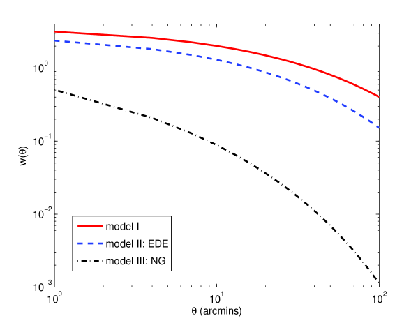
While both the EDE and non-Gaussian models generate higher S-Z power levels with respect to those predicted by the standard $\Lambda$CDM model, the levels of the A2PCF of S-Z clusters are lower in model II, and particularly so in model III, with respect to the corresponding levels predicted by model I, as illustrated in Fig. 3. The A2PCF of models I, II, and III peak at $w\sim 2,1,0.5$ at an angular separation of $1^{\prime}$, falling off towards levels of $w\sim 0.4,0.2,0.001$ at angular separation $100^{\prime}$. Also noticeable is the fact that the curve associated with model III has a greater slope than the corresponding slopes of models I and II. In order to understand these properties, it is useful to consider the redshift and mass dependence of the linear bias factor, which in the Gaussian case assumes the form (Mo & White 1996):

$$b(M,z)=1+\frac{\mu^{2}-1}{\delta_{c}(z)},$$ (7)

where $\mu\equiv\delta_{c}(z)/[\sigma_{M}(0)D_{+}(z)]$, $D_{+}(z)$ denotes the linear growth factor of density perturbations, and $\sigma_{M}(0)$ is the mass variance at $z=0$. Koyama, Soda, & Taruya (1999) generalised this expression to also address non-Gaussian models. Implementing their expression to the $\chi^{2}_{1}$ model, we have

$$b(M,z)=1+\frac{\mu^{2}-1}{\delta_{c}(z)[1+\sqrt{2}\mu]}.$$ (8)

The lower bias levels of massive haloes in non-Gaussian models are a consequence of the linear bias theory developed by Mo & White (1996), and were explored in detail by Amara & Refregier (2004) within the framework of the log-normal PDF. In fact, these authors showed that for a log-normal PDF with an excess probability in the $3\sigma$ tail of $\zeta\sim 10$, the corresponding bias factor is larger than the one predicted by the Gaussian model at halo masses $\gtrsim 5\cdot 10^{13}\,M_{\odot}\,h^{-1}$. Since the non-Gaussian model considered here has $\zeta\sim 16$, the mass scale at which the bias factor begins to be dominated by the corresponding Gaussian bias reduces to $\sim 10^{13}\,M_{\odot}\,h^{-1}$, which is the lower limit of our mass integral. It is therefore safe to assume that the relevant bias factor is lower than that of the Gaussian model within the entire mass range.

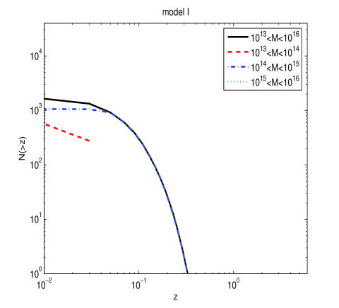
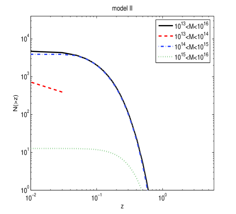
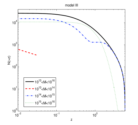
The properties of the A2PCF can be now easily explained by inspection of the functional dependence of the bias factor on mass and redshift. The bias factor increases with increasing mass, since the mass variance decreases monotonically with increasing mass. Additionally, the bias factor increases with increasing redshift since the critical density for collapse increases with increasing redshift, whereas the linear growth factor decreases with increasing redshift. These properties are common to all of the three models. The differences between the predictions of the 3 models arise either from the different evolution of $\delta_{c}(z)$ and $D(z)$ in model II, or the distinct functional form of the bias factor in model III. In model II, the magnitude of the bias factor is lower than in model I, in light of the lower and higher values of the critical density for collapse and linear growth factor, respectively (Fig. 5). This is reflected in the lower levels of the A2PCF in model II, with respect to model I. More striking are the differences between the predicitons of models I and III. As can be easily realized from equation (8), the bias is reduced owing to the addition of a larger than unity factor in the denominator of the second term, which is reflected in the substantially lower levels of the A2PCF. Note however, that the differences between the correlation levels of models I and III increase with increasing angular separation. At low angular separations both nearby and distant clusters contribute to the A2PCF by virtue of their relatively low mutual distances. Since the occurence of high-redshift, massive clusters, capable of generating the required flux limit, is substantially larger in model III, these contribute significanly to the correlation levels of model III at low angular separations, whereas the corresponding contribution in model I originates in clusters residing at lower redshifts. At higher angular separations, where correlations can only arise locally, a relative deficit of low redshift clusters appear in model III, as can be seen in Fig. 4, where we plot cumulative number counts of S-Z clusters (evaluated at a frequency of $353\,GHz$, with beam size of $5.1^{\prime}$, and flux detection limit $30\,mJy$). Indeed, if we compare the upper left-hand panel with the lower panel of Fig. 4, we may see that while (cumulative) cluster counts continue to increase in the redshift range $0.2\gtrsim z\gtrsim 0.01$ in model I, they level off at $z\lesssim 0.2$ in model III. This property of model III gives rise to the faster descent of the A2PCF, with respect to model I, at high angular separations.

Figure 3: The A2PCF of clusters calculated from their S-Z fluxes in models I (continuous), II (dashed), and III (dash-dotted), as a function of separation angle, $\theta$. The calculations were carried out for the $353\,GHz$ channel of the Planck/HFI experiment, with a beamsize of $5.1^{\prime}$ and a limiting flux of $30\,mJy$.

Figure 4: Cumulative number counts of S-Z clusters with fluxes exceeding $30\,mJy$ as a function of redshift. The calculations were carried out at a frequency of $353\,GHz$ and beam size $5.1^{\prime}$. Upper left- and right-hand panels and the bottom panel correspond to models I, II, and III, respectively. Continuous curves depict the contribution to the cumulative number counts in the entire mass range of $10^{13}M_{\odot}h^{-1}\leq M\leq 10^{16}M_{\odot}h^{-1}$; dashed, dash-dotted and dotted curves represent contributions from partial mass ranges, as indicated in the legend.

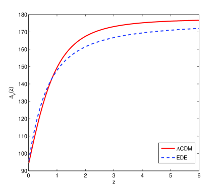
The results presented so far focused on the differences in S-Z power and angular correlation levels in the three models due to the respective mass functions and bias factors. Internal cluster properties relevant to the S-Z effect, such as virial size and the temperature and density of the intracluster gas, may be affected as well, as can be seen in the bottom panel of Fig. 5, where $\Delta_{v}(z)$, the overdensity (scaled to the critical density) at virialisation is plotted as function of redshift. However, the variation of $\Delta_{v}(z)$ among the models amounts to less than $4\%$, implying little change in the above cluster internal properties, particularly so in comparison with the major differences apparent in the mass function and bias parameter.

4 DISCUSSION

The reported low value of $\sigma_{8}$ inferred from the WMAP 3-year data implies a significantly reduced population of high-mass clusters of galaxies, as predicted by a Press & Schechter mass function based on a Gaussian density fluctuation field. With this low value it becomes even more difficult to attribute the CMB power excess measured with the CBI and ACBAR experiments at high multipoles to the (thermal) S-Z effect. The reason for this difficulty lies in the fact that the largest contribution to S-Z power comes from high-mass clusters, whose number density decreases steeply with decreasing $\sigma_{8}$. If indeed this excess is attributed to the S-Z effect, an enhanced massive cluster population at moderate and high redshifts is required. In this work we have studied the implications of two non-standard cosmological models on S-Z observables, specifically, the angular power spectrum, and A2PCF. The model based on a primordial density fluctuation field obeying $\chi^{2}_{1}$ statistics generates a more abundant population of massive clusters by virtue of higher probabilities for overdense regions at high redshifts. These collapse earlier and form cluster haloes, whereas the early quintessence model is characterized by earlier collapse owing to the higher linear growth factor and lower value of the critical density for collapse at high redshifts. Both models give rise to higher S-Z power levels, more so in the non-Gaussian model.

We note that the two non-standard models investigated here are by no means unique; for example, lower S-Z power is expected in non-Gaussian models based on $\chi^{2}_{m}$ statistics with $m>1$ due to less pronounced skewness (or non-Gaussianity) of the density field. Likewise, early quintessence models with higher early dark energy densities are likely to further slow down the evolution of the linear growth factor (reducing the value of $\delta_{c}$) and thus give rise to higher power levels. Conversely, the A2PCF of S-Z clusters in the EDE model, and to a significantly higher degree in the non-Guassian model, is manifested in reduced correlation levels with respect to those of the standard $\Lambda$CDM model, in particular at high angular separations.

EDE models with still larger quintessence densities at early times would enhance power levels and further blur the distinction between such models and non-Gaussian models. On the other hand, the A2PCF provides a more adequate test of the viability of these models. In this regard we mention the recent work of Magliocchetti et al. (2006), who report results from analysis of Spitzer Space Telescope observations that presumably provide evidence for strong clustering of a galaxy population at $z\sim 2$. According to Magliocchetti et al., these observations suggest that the detected objects are very massive proto-spheroidal galaxies, with number densities that are considerably higher than predicted by theory. If this is indeed the case, it adds to a list of other observational indications of enhanced massive objects lying at relatively high redshifts, among which are the detection of structures with high velocity dispersions at redshifts $\sim 4$ (Miley et al. 2004) and $\sim 2$ (Kurk et al. 2004), and the detection of protoclusters with masses lying in the range $2-9\cdot 10^{14}\,M_{\odot}$ associated with radio galaxies lying at $z>2$ (Venemans et al. 2006). All this observational evidence points to the presence of massive objects at high redshifts, which - as shown here - may be accounted for by either a non-Gaussian, or early quintessence models. If additional evidence (such as reported by Magliocchetti et al.) is found for strong clustering at $z\sim 2$, it will add further support for non-Gaussian models. It is important to stress that these observational results pointing to strong clustering of galaxies are not necessarily in conflict with the lower correlations found for the non-Gaussian model presented in the previous section. This is due to the fact that our calculations include the contribution to the A2PCF from clusters of galaxies alone, for which, as has been explained above, the (non-Gaussian) bias is lower than the corresponding Gaussian bias. At lower masses, such as galaxies, the bias is actually stronger in non-Gaussian models, and would yield higher levels of the A2PCF. Finally, it is noteworthy that the linear bias factor fails to describe the actual clustering on galaxy scales, since these are already considerably non-linear. Models admitting non-linear corrections exist (e.g. Peacock & Dodds 1996), but are not likely to alter the general behaviour of the bias parameter in the non-Gaussian and EDE models.

The non-standard cosmological models considered in this paper give rise to enchanced S-Z power by virtue of their impact on the cluster population. A legitimate question in this regard is whether internal cluster properties alone may be able to account for the apparent variance between the low $\sigma_{8}$ deduced from the WMAP 3-year data and the high-multipole CMB power excess observed by the ACBAR, CBI, and possibly BIMA experiments. We believe, however, that the answer to this question is negative. IC gas properties and their impact on the S-Z power spectrum have been extensively investigated in the literature; specifically, consequences of the gas mass fraction evolution (Majumdar 2001), isothermal, as well as polytropic temperature profiles (e.g. Komatsu & Seljak 2002), self-similar and entropy-driven models for the cluster core (Komatsu & Kitayama 1999), and the temperature-mass relation (SRS), were explored, and however significant differences were found, they are still incapable of settling the conflict. Recently, Roychowdhury, Ruszkowski, & Nath (2005) have explored the influence of AGN heating on groups and clusters of galaxies, motivated by the observed entropy excess in the IC gas. A consequence of this heating was shown to be a depletion of gas from the central regions of clusters, resulting in reduced S-Z power levels. Obviously, this cannot provide a remedy to the conflicting low $\sigma_{8}$ and high-multipole CMB power excess.

In conclusion we re-iterate the main result of our work: the mounting observational evidence for the presence of massive clusters already at relatively high redshifts cannot be easily reconciled with the Press & Schechter mass function (or variants thereof) in the standard $\Lambda$CDM cosmology with underlying Gaussian density fluctuation field. Non-Gaussian fields and early quintessence models may remove the inherent difficulty by allowing a more abundant population of massive clusters at high redshift. Moreover, such models give rise to enhanced S-Z power levels, which seem to be in better agreement with the CMB power excess at high multipoles observed by the CBI and ACBAR experiments. Future S-Z cluster catalogs will enable the construction of A2PCF from S-Z measurements, thereby providing an additional test for the viability of these models.

5 APPENDIX

Extension of the numerical computation of the S-Z angular power spectrum and A2PCF to EDE models necessitates a re-evaluation of several cosmological quantities that are affected by the presence of early dark energy. These include the (comoving) radial and angular diameter distances, the linear growth factor of density perturbations, the critical density for spherical collapse, and the overdensity at virialisation. This Appendix details the necessary modifications to the basic equations governing the redshift (or equivalently, the scale factor, $a$) dependence of these functions, and presents their numerical results.

The EDE model studied in this work is characterised by flat geometry, with an early quintessence density specified by the parameter $\Omega_{e}$, and an effective redshift-dependent coefficient of the equation of state given by

$$\overline{w}(z)=\frac{w_{0}}{1-[3w_{0}\log{(1+z)}]/(\log{\frac{1-\Omega_{e}}{\Omega_{e}}}+\log{\frac{1-\Omega_{m}}{\Omega_{m}}})},$$ (9)

where $w_{0}=w(z=0)$. By using the redshift scaling of the density of the dark energy component corresponding to this model,

$$\rho_{Q}=\rho_{Q_{0}}(1+z)^{3[1+\overline{w}(z)]},$$ (10)

in the Friedmann equation

$$\left(\frac{\dot{a}}{a}\right)^{2}=\frac{8\pi G}{3}(\rho_{m}+\rho_{Q}),$$ (11)

one obtains

$$\frac{\dot{a}}{a}\equiv H=H_{0}\left[\Omega_{m}(1+z)^{3}+(1-\Omega_{m})(1+z)^{3[1+\overline{w}(z)]}\right]^{1/2}.$$ (12)

1. Comoving radial and angular diameter distances

The comoving radial distance can be obtained from equation 12 as

$$r(z)=\frac{c}{H_{0}}\int_{0}^{z}\frac{dz^{\prime}}{\left[\Omega_{m}(1+z)^{3}+\Omega_{Q}(1+z)^{3[1+\overline{w}(z)]}\right]^{1/2}},$$ (13)

with $\Omega_{Q}=1-\Omega_{m}$, whereas the angular diameter distance is simply

$$d_{A}=\frac{r(z)}{1+z}.$$ (14)

2. Linear growth factor

The differential equation governing the evolution of the linear growth factor of density perturbations is

$$\frac{d^{2}\delta}{da^{2}}+\left[\frac{2}{a}-\frac{1}{2a}\frac{\Omega_{Q}a^{-3[1+\overline{w}(z)]}[1+3\overline{w}(z)]+\Omega_{m}a^{-3}}{\Omega_{Q}a^{-3[1+\overline{w}(z)]}+\Omega_{m}a^{-3}}\right]\frac{d\delta}{da}-\frac{3}{2}\frac{\Omega_{m}}{a^{5}}\frac{1}{\Omega_{Q}a^{-3[1+\overline{w}(z)]}+\Omega_{m}a^{-3}}\delta=0.$$ (15)

3. Critical density for spherical collapse

Using the Friedmann equations for both the spherical overdensity and the background manifold, and denoting by $a_{ta}$ and $R_{ta}$ the scale factor and radius of the spherical overdensity at turnaround, respectively, $\rho_{{Qb},{ta}}$, $\rho_{{mb},{ta}}$, and $\rho_{{mc},{ta}}$ the background density of the dark energy component, the background density of the matter component, and the collapsed density of the matter component at turnaround, respectively, we have

$$\left(\frac{\dot{R}}{R}\right)^{2}=\frac{8\pi G}{3}(\rho_{mc}+\rho_{Qc})-\frac{k}{R^{2}}$$ (16)

$$\left(\frac{\dot{a}}{a}\right)^{2}=\frac{8\pi G}{3}(\rho_{mb}+\rho_{Qb}),$$ (17)

where the curvature $k$ is assumed to vanish in our model, and the indexes $c$ and $b$ refer to collapsed and background components, respectively, the following differential equation may be obtained:

$$\left(\frac{dy}{dx}\right)^{2}=\frac{\zeta(y^{-1}-1)+\nu(y^{-1}R_{ta}^{3\overline{w}(R_{ta})}/R^{3\overline{w}(y\cdot R_{ta})}-1)}{x^{-1}+\nu x^{-1}a_{ta}^{3\overline{w}(a_{ta})}/(x\cdot a_{ta})^{3\overline{w}(x\cdot a_{ta})}},$$ (18)

with $x\equiv a/a_{ta}$, $y\equiv R/R_{ta}$, $\nu\equiv\rho_{{Qb},{ta}}/\rho_{{mb},{ta}}$, and $\zeta\equiv\rho_{{mc},{ta}}/\rho_{{mb},{ta}}=\left(R_{ta}/a_{ta}\right)^{-3}$. Since $x=0$ and $y=0$ at $t=0$, whereas $x=1$ and $y=1$ at turnaround, it is possible to recast equation 18 in the form

$$\int_{0}^{1}\frac{dy}{\left[\zeta(y^{-1}-1)+\nu(y^{-1}(a_{ta}\zeta^{-1/3})^{3\overline{w}(a_{ta}\zeta^{-1/3})}/(y\cdot(a_{ta}\zeta^{-1/3}))^{3\overline{w}(y\cdot(a_{ta}\zeta^{-1/3}))}-1)\right]^{1/2}}$$

$$=\int_{0}^{1}\frac{dx}{\left[x^{-1}+\nu x^{-1}a_{ta}^{3\overline{w}(a_{ta})}/(x\cdot a_{ta})^{3\overline{w}(x\cdot a_{ta})}\right]^{1/2}},$$ (19)

where we have used the relation $R_{ta}=a_{ta}\zeta^{-1/3}$. Equation (19) can be solved numerically to yield the sought value of $\zeta$, and the critical density for spherical collapse can then be found as (Zeng & Gao 2005a):

$$\delta_{c}=\frac{3}{5}a_{ta}^{-1}\left(\zeta^{1/3}+\nu\,a_{ta}\zeta^{-2/3}\right)D(a_{c}),$$ (20)

where $D(a_{c})$ is the linear growth factor at the time of collapse.

4. Overdensity at virialisation

The overdensity of the virialised matter component can be found by relating the background and collapsed matter densities at turnaround with their counterparts at the time of collapse:

$$\Delta_{v}=\frac{\rho_{mc,c}}{\rho_{mb,c}}=\frac{\rho_{mc,ta}}{\rho_{mb,ta}}\cdot\frac{\left(R_{ta}/R_{c}\right)^{3}}{\left(a_{ta}/a_{c}\right)^{3}}\equiv\zeta\cdot\lambda^{-3}\left(\frac{a_{c}}{a_{ta}}\right)^{3},$$ (21)

or if we are rather interested in the virialised overdensity in terms of the critical density at the time of collapse

$$\Delta_{v}^{*}=\frac{\rho_{mc,c}}{\rho{c,c}}=\Omega_{m}(a_{c})\cdot\Delta_{v},$$ (22)

where we have defined $\lambda\equiv R_{c}/R_{ta}$. It remains to specify this parameter. This can be done by requiring energy conservation at turnaround and virialisation, in conjunction with the virial theorem applied to the virialised phase of the collapsed overdensity. Before proceeding along this line, we remark that there is an ongoing debate regarding the assumption of energy conservation within the collapsing halo in models with dark energy featuring $w\neq-1$ (e.g. Basilakos & Voglis 2007, Zeng & Gao 2005b, Maor & Lahav 2005). In fact, Maor & Lahav show that in such models the assumption of energy conservation breaks down. Here we choose to ignore this issue, and use energy conservation as a zero order approximation. It is also of interest to note that according to Wang (2006), under certain conditions (namely, for $\nu/\zeta<0.01$), the problematics associated with energy conservation do not affect the virialisation process. Although this factor is somewhat larger in our adopted model, we believe that our results are not significantly affected by this ambiguity.

To proceed, the potential energy stored in the matter component of the spherical overdensity is the usual

$$U_{G}=-\frac{3GM^{2}}{5R},$$ (23)

whereas the potential energy associated with the dark energy in the spherical overdensity is (Horellou & Berge 2005)

$$U_{Q}=(1+3\overline{w})\rho_{Q}\cdot\frac{4\pi GM}{10}R^{2}.$$ (24)

At turnaround the spherical overdensity has only potential energy, while at virialisation it has both kinetic and potential energies:

$$(T+U)_{ta}=(T+U)_{c}.$$ (25)

Using the virial theorem, $T_{c}=-1/2U_{G}+U_{Q}$, so

$$\frac{1}{2}U_{G,c}+2U_{Q,c}=U_{G,ta}+U_{Q,ta}.$$ (26)

Substitution of equations (23) and (24) in equation (26) (and performing some algebraic manipulations) leads to the following equation:

$$\frac{R_{ta}}{R_{c}}=\frac{4\pi[1+3\overline{w}(a_{ta})]\rho_{Q,ta}R_{ta}^{3}-6M}{8\pi[1+3\overline{w}(a_{c})]\rho_{Q,c}R_{c}^{3}-3M}.$$ (27)

Using the fact that the mass can be represented by either $M=4\pi/3\rho_{mc,ta}R_{ta}^{3}$ or $M=4\pi/3\rho_{mc,c}R_{c}^{3}$, this can be written as

$$\frac{R_{ta}}{R_{c}}=\frac{[1+3\overline{w}(a_{ta})]\frac{\Omega_{Q,ta}}{\Omega_{mb,ta}}\frac{1}{\zeta}-2}{2[1+3\overline{w}(a_{c})]\frac{\Omega_{Q,c}}{\Omega_{mb,c}}\left(\frac{a_{ta}}{a_{c}}\right)^{3}\left(\frac{R_{c}}{R_{ta}}\right)^{3}\frac{1}{\zeta}-1}.$$ (28)

Given the collapse scale factor $a_{c}$, or, alternatively, the collapse redshift $z_{c}$, all of the density parameters appearing in this equation can be found. Substituting $\lambda\equiv{R_{c}}{R_{ta}}$, the last equation can be written as

$$\frac{n_{1}-2}{2n_{2}\lambda^{3}-1}=\frac{1}{\lambda},$$ (29)

or

$$2n_{2}\lambda^{3}-(n1-2)\lambda-1=0,$$ (30)

where $n_{1}\equiv[1+3\overline{w}(a_{ta})]\zeta^{-1}(\Omega_{Q,ta}/\Omega_{mb,ta})$, and $n_{2}\equiv[1+3\overline{w}(a_{c})]\zeta^{-1}(\Omega_{Q,c}a_{ta}^{3})/(\Omega_{mb,c}a_{c}^{3})$ can all be evaluated given the collapse redshift. The solution for $\lambda$ should obviously lie in the range $0\leq\lambda\leq 1$.

Numerical results for the linear growth factor, critical overdensity for collapse, and overdensity at virialisation in the EDE model are compared with the corresponding results for the standard $\Lambda$CDM model in Fig. 5.

Figure 5: Numerical results for the linear growth factor, critical density for spherical collapse, and the overdensity at virialisation are illustrated in the upper left-hand, upper right-hand, and bottom panels, respectively, for models I (continuous) and II (dashed).

6 ACKNOWLEDGMENT

We thank the referee for useful comments. Work at Tel Aviv University is supported by a grant from the Israel Science Foundation.

7 REFERENCES

Amara A., Refregier A., 2004, MNRAS  , 351, 375

Avila-Reese V., Colin P., Piccinelli G., Firmani C., 2003, ApJ  , 598, 36

Bardeen J.M., Bond J.R., Kaiser N., & Szalay A.S., 1986,ApJ  , 304,15

Bartelmann M., Doran M., Wetterich C., 2006, Astron. Astrophys.  , 454, 27

Basilakos S., Voglis N., 2007, MNRAS  , 374, 269

Caldwell R.R., Doran M., Müller C.M., Schäfer G., Wetterich C., 2003, ApJ  , 591, L75

Coles P., Barrow J.D., 1987, MNRAS  , 228, 407

Cooray A., 2000, Phys. Rev. D.  , 62, 103506

Dawson K.S., Holzapfel W.L., Carlstrom J.E., Joy M., LaRoque S.J., Miller A.D., Nagai D., 2002, ApJ  , 581, 86

Doran M., Lilley M., Schwindt J., Wetterich C., 2001a, ApJ  , 559, 501

Doran M., Schwindt J., Wetterich C., 2001b, Phys. Rev. D.  , 64, 123520

Evrard A.E. et al., 2007, preprint (astro-ph/0702241)

Ferreira P.G., Joyce M., 1998, Phys. Rev. D.  , 58, 023503

Horellou C., Berge J., 2005, MNRAS  , 360, 1393

Komatsu E., Kitayama T., 1999, ApJ  , L1

Komatsu E., Seljak U., 2002, MNRAS  , 336, 1256

Komatsu E. et al., 2003, Ap. J. Supp.  , 148, 119

Koyama K., Soda J., Taruya A., 1999, MNRAS  , 310, 1111

Kuo C.L. et al., 2004, ApJ  , 600, 32

Magliocchetti M., Silva L., Lapi A., De Zotti G., Granato G.L., Fadda D., 2006, preprint (astro-ph/0611409)

Majumdar S., 2001, ApJ  , L7

Maor I., Lahav O., 2005, J. Cosmo. Astro. Phys.  , 7, 3

Matarrese S., Verde L., Jimenez R., 2000, ApJ  , 541, 10

Mathis H., Diego J.M., Silk J., 2004, MNRAS  , 353, 681

Mo H.J., White S.D.M., 1996, MNRAS  , 282, 347

Peacock J.A., Dodds S.J., 1996, MNRAS  , 280, 19

Peebles P.J.E., 1997, ApJ  , 483, L1

Peebles P.J.E., 1999a, ApJ  , 510, 523

Peebles P.J.E., 1999b, ApJ  , 510, 531

Press W.H., Schechter P., 1974, ApJ  , 187, 425

Readhead A.C.S. et al., 2004, ApJ  , 609, 498

Refregier A., Teyssier R., 2002, Phys. Rev. D.  , 66, 043002

Robinson J., Baker J.E., 2000, MNRAS  , 311, 781

Robinson J., Gawiser E., Silk J., 2000, ApJ  , 532, 1

Roychowdhury S., Ruszkowski M., Nath B.B., 2005, ApJ  , 634

Sadeh S., Rephaeli Y., Silk J., 2006, MNRAS  , 368, 1583

Spergel D.N., Bean R., Doré O., et al., 2006, preprint (astro-ph/0603449)

Venemans B.P., Rottgering H.J.A., Miley G.K., van Breugel W.J.M., De Breuck C., Kurk J.D., Pentericci K., Stanford S.A., Overzier R.A., Croft S., Ford H., 2006, preprint (astro-ph/0610567)

Wang P., 2006, ApJ  , 640, 18

Wetterich C., 2004, Phys. Lett. B.  , 594, 17

Zeng D-f, Gao Y-h, 2005a, preprint (astro-ph/0412628)

Zeng D-f, Gao Y-h, 2005b, preprint (astro-ph/0505164)