Finite-size effects in roughness distribution scaling
Abstract
We study numerically finite-size corrections in scaling relations for roughness distributions of various interface growth models. The most common relation, which considers the average roughness as scaling factor, is not obeyed in the steady states of a group of ballistic-like models in dimensions, even when very large system sizes are considered. On the other hand, good collapse of the same data is obtained with a scaling relation that involves the root mean square fluctuation of the roughness, which can be explained by finite-size effects on second moments of the scaling functions. We also obtain data collapse with an alternative scaling relation that accounts for the effect of the intrinsic width, which is a constant correction term previously proposed for the scaling of . This illustrates how finite-size corrections can be obtained from roughness distributions scaling. However, we discard the usual interpretation that the intrinsic width is a consequence of high surface steps by analyzing data of restricted solid-on-solid models with various maximal height differences between neighboring columns. We also observe that large finite-size corrections in the roughness distributions are usually accompanied by huge corrections in height distributions and average local slopes, as well as in estimates of scaling exponents. The molecular-beam epitaxy model of Das Sarma and Tamborenea in dimensions is a case example in which none of the proposed scaling relations works properly, while the other measured quantities do not converge to the expected asymptotic values. Thus, although roughness distributions are clearly better than other quantities to determine the universality class of a growing system, it is not the final solution for this task.
pacs:
68.35.Ct, 81.15.Aa, 05.40.-aI Introduction
In order to understand the basic mechanisms of a growth process, it is a common practice to associate it to a certain universality class barabasi ; krug . This is usually done with the calculation of scaling exponents of surface roughness and assuming that Family-Vicsek scaling is valid fv (with a suitable generalization when anomalous scaling holds). However, huge corrections to scaling make this calculation difficult in finite-size systems, both for simulation work and for the analysis of images of real surfaces. These problems and the interest in finding more universal properties of growth processes motivated recent studies of other quantities, such as the distributions of surface roughness foltin ; racz ; antal ; marinari1 . Most efforts were devoted to calculation of those distributions in steady states (roughness saturation), but the comparison of distributions obtained under conditions that parallel experimental work (the so-called window boundary conditions) is also a promising tool moulinet ; rosso ; localKPZ ; santachiara .
It is expected that roughness distributions scale as
| (1) |
where is the probability density of the roughness of a given configuration to lie in the range , is a scaling function, the overbars denote spatial averages and the angular brackets denote configurational averages. Eq. (1) is usually obtained in analytical work, such as in the calculation of distributions for -noise interfaces antal . An alternative scaling relation is
| (2) |
where
| (3) |
is the root mean square (rms) deviation of .
It is reasonable to claim that comparison of full roughness distributions is better than the calculation of one or two exponents to determine the class of a growth process. However, these distributions may also be deviated from the expected scaling relations by finite-size corrections. For instance, finite-size data of some models in the Kardar-Parisi-Zhang (KPZ) class kpz show small deviations from relation (1), while good data collapse of numerical data for different lattice sizes is obtained with relation (2) distrib . The advantage of a scaling relation equivalent to (2) was also illustrated in the study of maximal height distributions (MHD) of signals gyorgyi . Moreover, the leading corrections to scaling in MHD of some one-dimensional solid-on-solid models were analytically predicted and numerically confirmed in Ref. schehr , which clearly shows that such corrections are not related to low accuracy of simulation data. The presence of huge scaling corrections may be much worse in distributions of other quantities, such as height distributions chin ; shim ; marinari ; kpz2d .
For the above reasons, investigation on the failure of finite-size scaling of roughness distributions is essential to ensure their reliability for comparison with real or model systems. Moreover, understanding the reasons for the failure of an scaling relation and the advantages of other ones may also be helpful to find the form of the main finite-size corrections and to propose alternative methods of analysis. One particularly important case is KPZ growth in dimensions, since this class contains many models with large corrections to scaling of the average roughness, such as ballistic deposition (BD) and Eden growth, as well as a large number of applications (see e. g. Refs. krim ; miettinen ; tsamouras ).
The aim of this work is to study finite-size corrections in roughness distribution scaling by analyzing numerical simulation data of various interface growth models and to discuss the possible relations with other quantities that characterize those interfaces. The numerical approach is essential to study the three-dimensional systems considered here, as well as some two-dimensional systems (the usual systems where analytic work is possible are Gaussian interfaces).
First, we will study a group of ballistic-like models where the deviations from relation (1) are much larger than those previously found in other models distrib . This means that no evidence on their universality class can be obtained by assuming that scaling relation. On the other hand, good collapse of large systems data is obtained with Eq. (2), which shows that they are actually in the KPZ class. Moreover, we successfully propose an alternative scaling relation accounting for the effect of the intrinsic width, which is a constant correction term previously included in the scaling of the average roughness stauffer ; kertesz . This shows how the main finite-size corrections may be extracted from roughness distribution scaling. However, we discard the usual interpretation that the intrinsic width is a consequence of high surface steps by analyzing data of restricted solid-on-solid (RSOS) models, where this correction is not present. Instead, we observe that the deviations from finite-size scaling in the roughness distributions are usually accompanied by significant finite-size dependence of dimensionless amplitude ratios of moments of height distributions, as well as of scaling exponents and average local slopes. This conclusion is not restricted to KPZ systems, as shown in the analysis of the molecular-beam epitaxy model of Das Sarma and Tamborenea (DT) dt in dimensions, which is well-known for the slow convergence of numerically estimated exponents tamborenea ; lanczycki . Indeed, for this model none of the proposed scaling relations is able to produce good collapse of small systems data.
Although we are not able to determine all the reasons for the failure of scaling relations in a given universality class, we will show how deviations in different quantities are connected and will suggest alternative methods of analysis. This may be helpful not only in future work on complex models and real systems, but also to search for models with minimal finite-size effects, e. g. following the ideas of Ref. ghaisas . Anyway, an important conclusion is that roughness distributions are actually superior to other quantities for a reliable search of the universality class of a growing system, although it is not the final solution for all models.
The rest of this work is organized as follows. In Sec. II we discuss the above scaling relations and propose an alternative one for cases where intrinsic width is expected. In Sec. III we present the discrete models analyzed in the subsequent Sections and the equations defining their universality classes. In Secs. IV, V and VI, we discuss the finite-size effects in the roughness distributions, the role of local slopes and the finite-size effects in the height distributions, respectively. In Sec. VII we summarize our results and present our conclusions.
II Basic properties of scaling functions
If the scaling relation (1) holds, the function is a function of the variable . The moment of order of this function is defined as , so that the first moments are given by
| (4) |
This means that any finite-size dependence of the ratio (between the average square roughness and its rms fluctuation) will lead to a finite-size dependence of the second moment. However, in the scaling relation (2), is a function of the variable , so that the first moments of are
| (5) |
This means that the finite-size dependence of do not lead to deviations in the second moment of this scaling function, leaving possible corrections to the third moment.
In works based on data collapse methods, the fluctuations in the first few moments of a scaling function are the ones most easily related to visual deviations of the plots of data from different system sizes. Consequently, scaling relation (2) is expected to be better than (1) by avoiding that finite-size effects are reflected in its second moment. This was already observed for some KPZ models in dimensions in relatively small system sizes distrib . Recent work on maximal height distributions of signals also illustrated this feature and stressed the fact that finite-size scaling of the higher cumulants was related to the deviations gyorgyi .
The knowledge of the particular properties of a growth model is certainly important to guide the proposal of suitable scaling relations. For instance, this was the case of a recent work on elastic lines in random environments, in which the scaling relation (1) was generalized to incorporate time and temperature effects bustingorry . Here, we will consider a series of ballistic-like models whose deposits contain holes and overhangs, among other steep features, thus our approach is based on properties of related models.
Simulation work on models which produce deposits with holes and overhangs, such as the Eden model, suggested that the leading correction to the scaling of the average squared roughness is a constant term stauffer ; kertesz ; tammaro ; chavez ; moro . The time evolution of the average squared roughness, starting from a flat interface, obeys
| (6) |
where is a constant called the intrinsic width, is the roughness exponents and is the dynamic exponent. The usual interpretation of relation (6) is that the first term at the right-hand side (the original Family-Vicsek relation fv ) is associated with fluctuations of all wavelengths, while the intrinsic width is thought to be related to short wavelength features, represented by overhangs, holes and high steps at the film surface - see e. g. Refs. kertesz ; tammaro .
The present work is only concerned with steady state properties, where in Eq. (6) and the saturation roughness [] scales as
| (7) |
with constant. Large values of are responsible for remarkable deviations of finite-size estimates of exponent from its asymptotic value. However, numerical work on ballistic-like models show that finite-size corrections to the scaling of are smaller than the corrections in sigma .
These results lead us to propose that, for the ballistic-like models, the roughness of a given interface configuration is a sum of a fluctuating value, which is distributed according to the universality class of the model, and a constant contribution, which is the intrinsic width. Following this reasoning, we change relation (1) by subtracting a constant from and :
| (8) |
Here must be viewed as a fitting constant and is a scaling function. The first moments of the function , where , are
| (9) |
If our assumptions are correct and is chosen to match the intrinsic width , then the finite-size dependence of the second moment will be cancelled, or at least it will be greatly reduced. Consequently, the quality of a data collapse plot will be similar to that based on Eq. (2). Certainly this proposal has to be validated by numerical (or eventually analitic) work, and it is also important to notice that it is independent on the particular interpretation given to the intrinsic width.
III Discrete growth models and universality classes
The discrete models analyzed in this paper are the original BD model, the RSOS model, a conserved RSOS model, the grain deposition models and the DT model. In all cases, deposition begins with a flat substrate.
In BD, each incident particle is released from a randomly chosen position above the deposit, follows a trajectory perpendicular to the substrate and sticks upon first contact with a nearest neighbor occupied site vold ; fv .
In the RSOS model kk ; alanissila , the incident particle can stick at the top of a column only if the differences of heights of all pairs of neighboring columns do not exceed after aggregation. Otherwise, the aggregation attempt is rejected. In this work, results for , and will be presented.
The original conserved RSOS model (CRSOS) was proposed in Ref. crsos1 , but here we will consider an extension of that model that has the same symmetries and, consequently, belong to the same universality class. In this generalized CRSOS model crsos2 , hereafter simply called CRSOS, if the column of incidence does not obey the above condition for aggregation, with , then the incident particle executes random walks among neighboring columns until finding a position where it is satisfied and aggregation can occur.
In the model dt , the arriving particle sticks at the top of the column of incidence if it has one or two lateral neighbors at that position. Otherwise, the neighboring columns are consulted and if one of them satisfies that condition, then the incident particle aggregates at that point. However, if no neighboring column satisfies the condition, then the particle sticks at the top of the column of incidence, and if both neighboring columns satisfy the condition, then one of them is randomly chosen.
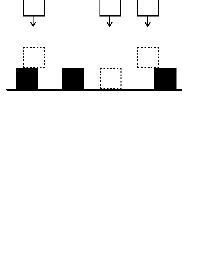
The grain deposition models studied here were introduced in Ref. graos for the study of a crossover in local roughness scaling similar to experimental systems. They are defined in a simple cubic lattice where the length unit is the lattice parameter. The grains have cubic shapes and lateral size . They sequentially incide perperdicularly to an initially flat substrate, with two of their faces parallel to the substrate. The incident grain permanently aggregates to the deposit when its bottom touches a previously aggregated grain (thus, there is no lateral aggregation). The process is shown in Fig. 1. Here we will simulate the model with grain sizes ranging from to . Despite the different aggregation rules, the grain deposition models and the BD model form the group to which hereafter we will refer as ballistic-like models.
The symmetries of the ballistic-like models and of the RSOS models indicate that they are in the KPZ universality class (see e. g. the discussion in Ref. hagston , in which the continuous description of the growth process is provided by the KPZ equation
| (10) |
Here, and are constants, is a Gaussian noise with zero mean and variance , with constant, and is the dimension of the substrate. In the following sections, we will study those models in dimensions (in dimensions, some exact results and highly accurate numerical results are already available).
The DT and the CRSOS models in dimensions are in the class of the nonlinear fourth order growth equation predota ; kotrla ; huang ; park
| (11) |
where and are constants. This is also known as Villain-Lai-Das Sarma (VLDS) equation villain ; laidassarma , and the discrete models are said to belong to the VLDS class. The DT model is particularly interesting in dimensions due to the presence of strong finite-size corrections which leads to exponents estimates far from the VLDS values (although noise reduction methods are able to provide estimates closer to the VLDS ones punyindu ).
For all models, only steady state properties will be studied in this work. The roughness distributions are typically obtained from to different configurations, and height distributions from a number of configurations which is larger by a factor (the square of the lattice size).
IV Scaling of roughness distributions
In order to compare the roughness distributions of the above models, we use two of them as representatives of their growth classes: the RSOS model with , whose distribution hereafter will be referred as the RSOS/KPZ one ( dimensions, ), and the CRSOS model with , whose distribution hereafter will be referred as the CRSOS/VLDS one ( dimensions, ). The use of these models data as standards is possible because previous work have already shown that they have very small finite-size dependence distrib .
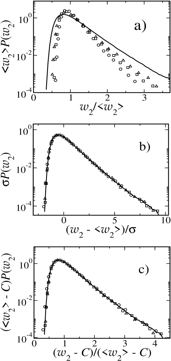
The original BD model illustrates the need of choosing a suitable scaling relation for the analysis of roughness distributions from small system sizes. In Figs. 2a, 2b and 2c we show its steady state distributions in dimensions obtained from to and scaled according to Eqs. (1), (2) and (8), respectively. For comparison, the RSOS/KPZ scaled distributions are also shown. In Fig. 2c, is used to match the peaks of the curves for BD and for RSOS/KPZ.
It is clear that the scaling with the rms fluctuation (Eq. 2) is superior if compared with the scaling with Eq. (1). Indeed, there is no data collapse in Fig. 2a, thus that plot is unable to confirm the KPZ scaling of the BD model. From the discussion of Sec. 2, the deviations may be related to finite-size corrections in the ratio , and our estimates of for different sizes confirm this large size-dependence.
However, the quality of the data collapse using Eq. (8) is similar to the one using Eq. (2). This result suggests that the assumptions leading to the proposal of Eq. (8) are reasonable, i. e. the roughness of each configuration is a constant plus a KPZ-distributed fluctuating part (Sec. II). It also gives an estimate of the intrinsic width, which is the constant (Fig. 2c).
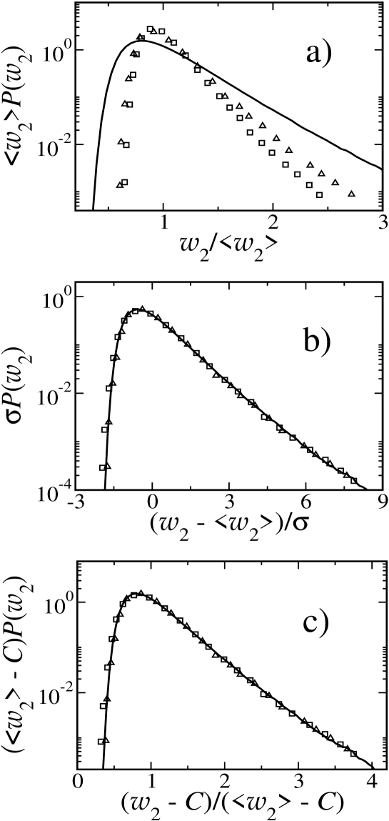
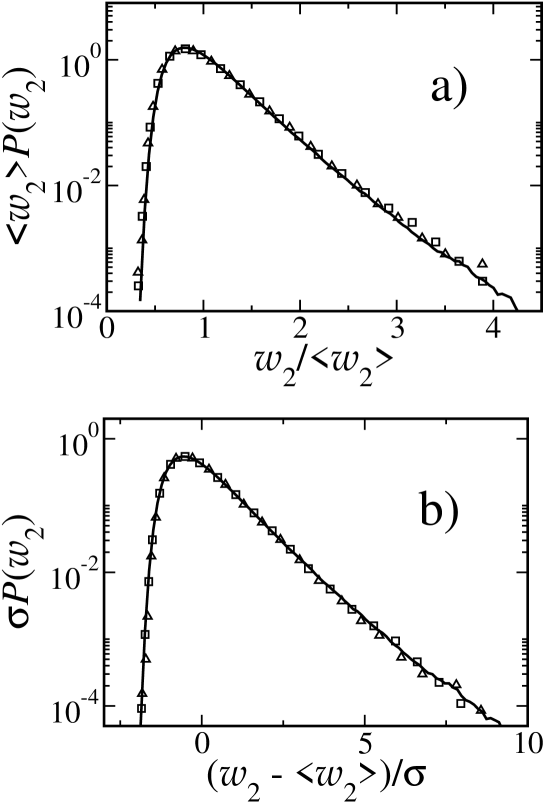
The scaled distributions of the grain deposition model with in lattice sizes and are shown in Figs. 3a, 3b and 3c, considering Eqs. (1), (2) and (8), respectively. The RSOS/KPZ distribution is also shown. Deviations from the scaling relation (1) are also large here, but using Eqs. (2) and (8) we obtain good data collapse with those large lattice sizes. Similar results were obtained with an extended model where the grains could have Poisson-distributed sizes, with an average size (the aggregation mechanism was the same of Fig. 1).
In BD and in this grain deposition model we observe deviations from data collapse with sizes smaller than those shown in Figs. 3a-c. The deviations for a certain lattice size become smaller when the grain size decreases, thus good data collapse is obtained for intermediate values of ( to ) with lattice sizes intermediate between those in Figs. 2a-c and 3a-c. Typically, significant deviations appear only for ( for BD), probably due to further corrections to scaling, whose effects are reduced as increases.
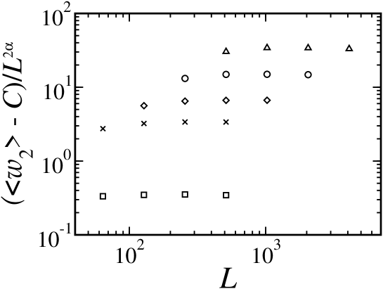
Our results for this group of ballistic-like models suggest that the roughness is actually distributed in a KPZ-like form except for an additional constant, which may be interpreted as the intrinsic width. Additional support to the constant correction term in the scaling of (Eq. 7) is given in Fig. 4, where we plot versus , using marinari ; kpz2d and the values of obtained from collapse of roughness distributions. The saturation value of for each model gives an estimate of the amplitude in Eq. (7). These estimates and the correction constants are shown in Table I, where we also present the corresponding values of both terms on the right-hand side of Eq. (7) for the largest lattice size used for each model (). The ratios between the leading correction () and the dominant term are very large for all model, in some cases exceeding , which quantitatively confirm the strong finite-size effects.
However, it is important to notice that the scaling with Eq. (8) advances over Eq. (2) because it not only confirms the universality class of the model (by data collapse) but also provides evidence on the leading finite-size correction to the roughness scaling. These results also advance over previous work where the intrinsic width was identified only as a correction to scaling of the average roughness stauffer ; kertesz ; tammaro ; chavez ; moro .
The intrinsic width is usually associated to steep surface features, such as large local slopes, holes and overhangs. In order to test this hypothesis, it is interesting to consider other models which also have large local slopes. This is the case, for instance, of the RSOS models with large .
In Figs. 5a and 5b we show the roughness distributions for the RSOS models with and scaled according to Eqs. (1) and (2), respectively. Both plots show excellent data collapse with very small lattice sizes, such as . Thus, there is no correction term similar to the intrinsic width or, equivalently, in Eq. (8) for the RSOS models.
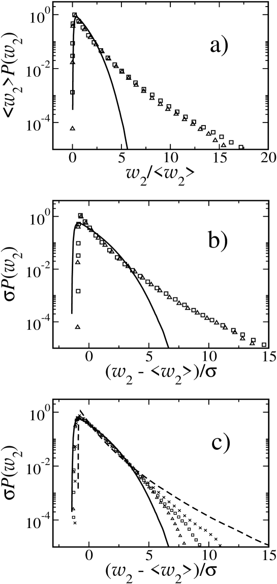
Finally, we analyze the DT model in dimensions. In Figs. 6a and 6b we show the roughness distributions for that model in lattice sizes and , scaled according to Eqs. (1) and (2). No significant finite-size effect is found in the scaling with the fluctuation (Fig. 6b). However, both plots show that the distribution of the DT model is very different from the CRSOS/VLDS distribution in dimensions () distrib . Moreover, there is no evidence that the former will converge to the CRSOS/VLDS curve as increases.
We observe the same large deviations when the DT distributions are scaled according to Eq.(8) for several values of the constant . Thus, the assumption of an intrinsic width is not sufficient to represent the main finite-size effects in that model, at least in the accessible range for simulation, which is .
However, previous work showed that simulation of noise-reduced DT models provides estimates of scaling exponents closer to the VLDS values punyindu . Thus, we also calculated the DT distributions using noise-reduction parameters , and . Here, is the number of times that a certain column has to be chosen for aggregation of a new particle before the aggregation actually takes place punyindu . In Fig. 6c we show the scaled distributions for these models in , which converge to the CRSOS/VLDS curve as increases (although reasonable data collapse is not obtained in the tails).
This noise-reduction scheme is not expected to change the universality class of the process because symmetries are preserved (see e. g. the discussion in Ref. hagston ). Thus, the above changes in the distributions when the parameter is increased (Fig. 6c) are evidence that the asymptotic behavior of the DT distribution was not attained yet. Consequently, the above discrepancies with the CRSOS/VLDS curve do not mean that the DT model does not belong to the VLDS class, but only that the finite-size effects on the roughness distributions have much more complex forms than those suggested here. Indeed, we recall that Ref. predota derived the VLDS equation from the master equation of the DT model in dimension.
In the following Sections, we will show that finite-size corrections obtained here in the roughness distributions are accompannied by corrections in other quantities.
V The role of the local slopes
Here we characterize the interfaces at small lengthscales by the average squared height difference between nearest neighbor columns, , also calculated at the steady states. Our main aim is to test the hypothesis that the intrinsic width is related to local height fluctuations of the interface.
In the ballistic-like models, has a significant finite-size dependence for small lattice sizes. However, it is approximately constant in the largest lattice sizes analyzed for each in Sec. III (the same sizes used to collapse the roughness distributions). However, in the RSOS models attains a saturation value for very small system sizes.
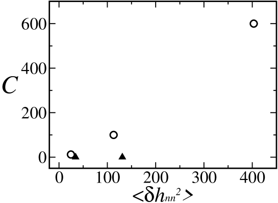
In Fig. 7 we plot the correction term obtained in the scaling with Eq. 8 (i. e. the intrinsic width) as a function of the large value of for both groups of models. The result for the ballistic-like models could naively suggest that the intrinsic width was only related to local height fluctuations. However, the result for the RSOS models show this interpretation is not valid in general: in that case and the values of are in the same range of those for ballistic-like models with .
In the DT model in dimensions, we observe a rapid increase of the average local slope with the lattice size: for , for , and for . A comparison with for the other models shown in Fig. 7 is not possible because we are not able to perform a reliable extrapolation of these data to . On the other hand, these data confirm that the DT model is very far from its asymptotic limit (the continuum VLDS model) in this range of lattice sizes.
The above results suggest that the presence of large fluctuations at small lengthscales is insufficient to explain the intrinsic width as the main correction term of roughness scaling in the ballistic-like models, since this is also a property of models which have much weaker scaling corrections (the RSOS ones). On the other hand, we observe that finite-size effects on roughness distributions are accompannied by the same type of effect on .
VI Finite-size effects in height distributions
Finite-size effects in height distributions are typically larger than those in roughness distributions, as illustrated for KPZ models in Ref. localKPZ . Thus, in order to study finite-size effects on steady state height distributions, the best procedure is to compare their skewness and kurtosis in different lattice sizes (other previous works which aimed at characterizing height distributions also focused on those quantities - see e.g. Refs. chin ; shim ; marinari ; kpz2d ). They are defined from the moments of the height distributions, , as
| (12) |
and
| (13) |
The sign of the skewness indicates which type of singular feature is dominant at the interface: deep valleys or grooves lead to negative , while sharp peaks give positive . In KPZ models the sign of is the same of the coefficient of the nonlinear term of the corresponding KPZ equation (see e. g. the discussion in Ref. kpz2d ). Thus, since ballistic-like models correspond to positive and RSOS models to negative , we must compare values of from the former with from the latter.
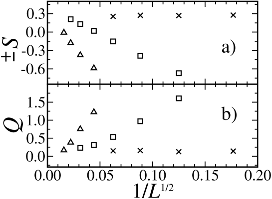
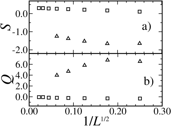
In Figs. 8a and 8b we show and versus , respectively, for BD, for the grain deposition model with and for the RSOS model with ( only for the RSOS model). Data for BD in the largest sizes were extracted from Ref. kpz2d . In Figs. 8a and 8b, the variable was used in the abscissa because it is the one which provides the best linear fits among other variables of the form , with one digit variation in . Since the asymptotic values of and are not known exactly, as well as their finite-size corrections, such numerical extrapolations are necessary.
We observe very weak finite-size corrections in the RSOS data, so that a simple extrapolation procedure to () leads to an asymptotic estimate of in agreement with the best known value of the KPZ class marinari ; kpz2d . However, there are large finite-size corrections in the data for the BD model. It is remarkable that up to , the skewness of BD is negative, while the values for larger are positive. The finite-size dependence of the data for the grain deposition model is much stronger: only for the skewness crosses over from negative to positive values.
The change in sign of of the ballistic-like models shows that the typical steady state configurations for small are very different from the typical ones for large . In other words, the steady states for small are not representative of the asymptotic limit of the model (large and ), which is the KPZ limit. For the grain deposition model with , even the steady state for has and, consequently, is very far from the KPZ limit.
Despite these problems, the data for the BD ballistic-like models indicate that is positive when . Asymptotic estimates (not very accurate) of can be obtained from extrapolations of those data; they are not very distant from the best known values for KPZ in dimensions. However, the finite-size effects on roughness distributions are certainly smaller than those found in height distributions. Indeed, the good data collapse in Figs. 2b, 2c, 3b and 3c is reflected in values of skewness (of the roughness distributions) close to the RSOS/KPZ curve.
The analysis of the kurtosis of the above models (Fig. 8b) leads to the same conclusions, although there the finite-size effects are much larger, as well as the error bars of the data.
The values of and for the DT and the CRSOS models are shown in Figs. 9a and 9b as a function of . They were estimated up to for the DT model (this work) and up to for the CRSOS model (Ref. crsos2 ), with a relatively low accuracy for the largest data. Here the variable in the abscissa was chosen by analogy with Fig. 8, but not for extrapolation purposes.
The asymptotic skewness of the VLDS class, , can be obtained from extrapolation of the CRSOS data to crsos2 . However, it is clear that the data for the DT model in Fig. 9a do not converge to the same value, even if the sign of is changed (the actual sign of is related to that of in Eq. 11). There is also no evidence that the kurtosis of the DT model will converge to the same value of the CRSOS model. Thus, the height distributions of the DT model up to are not representative of the VLDS class, even if we account for simple finite-size corrections.
The overall conclusion from the above results is that small or large finite-size corrections are simultaneously present in roughness and height distributions, but the convergence of roughness distributions to the asymptotic limit is certainly much better when it occurs, as illustrated with the ballistic-like models. The amplitude ratios of height distributions are interesting to show that, when the corrections are large, the finite-size configurations of hills and valleys are not representative of the universality class of the model. We are not able to explain why the roughness distributions (for large ) represent the correct class of the model when the height distributions do not, but certainly there is no contradiction in this finding because we are comparing distributions of local and global quantities, whose scaling properties may be very different.
VII Conclusion
For various interface growth models, height and roughness distributions and average square neighboring heights differences were numerically calculated in the steady states, in order to analyze their finite-size effects.
First, we considered a group of ballistic-like deposition models in which the most typical scaling relation for roughness distributions (Eq. 1) fails to provide collapse of finite-size systems data. On the other hand, good data collapse was obtained with a scaling relation involving the roughness fluctuation (Eq. 2) and with an alternative relation which includes the effect of the intrinsic width. This shows that this constant term is the main correction to the asymptotic KPZ distribution, thus extending previous work which suggested that quantity only as a correction to the scaling of the average roughness. The comparison with other models with large (the RSOS ones) show that the average local slope is not sufficient to explain the intrinsic width, in contrast to previous interpretation. Height distributions for those models also show strong finite-size effects, although results for sufficiently large lattice sizes indicate convergence of amplitude ratios to the expected asymptotic values.
We also studied the model of Das Sarma and Tamborenea (DT) in dimensions. Its roughness distributions up to size are very different from the ones representative of the asymptotic VLDS class. Strong finite-size effects are also observed in skewness and kurtosis of height distributions and in , with no evidence of convergence to reliable asymptotic values.
Our results show that the deviations from finite-size scaling in the roughness distributions are usually accompanied by significant finite-size dependence of dimensionless amplitude ratios of moments of height distributions and of average local slopes. One important point is that this conclusion is not restricted to the KPZ class. The analysis of simple quantities, such as , is useful to search for finite-size effects and may reveal slow convergence to a continuum limit. In some situations (e. g. the DT model here), this convergence may be so slow that no one of the quantities analyzed here are able to show the correct class of the growth process. In the other cases, roughness distributions are certainly better than other quantities (including scaling exponents) to classify the process.
Acknowledgements.
TJO acknowledges support from CNPq and FDAAR acknowledges support from CNPq and FAPERJ (Brazilian agencies).References
- (1) A.L. Barabási and H.E. Stanley, Fractal concepts in surface growth (Cambridge University Press, Cambribge, England, 1995).
- (2) J. Krug, Adv. Phys. 46, 139 (1997).
- (3) F. Family and T. Vicsek, J. Phys. A 18, L75 (1985).
- (4) G. Foltin, K. Oerding, Z. Rácz, R. L. Workman, and R. K. P. Zia, Phys. Rev. E 50 (1994) R639.
- (5) Z. Rácz and M. Plischke, Phys. Rev. E 50 (1994) 3530.
- (6) T. Antal, M. Droz, G. Györgyi, and Z. Rácz, Phys. Rev. E 65 (2002) 046140.
- (7) E. Marinari, A. Pagnani, G. Parisi, and Z. Rácz, Phys. Rev. E 65, 026136 (2002).
- (8) S. Moulinet, A. Rosso, W. Krauth, and E. Rolley, Phys. Rev. E 69, 035103(R) (2004).
- (9) A. Rosso, W. Krauth, P. Le Doussal, J. Vannimenus, and K. J. Wiese, Phys. Rev. E 68, 036128 (2003).
- (10) T. Paiva and F. D. A. Aarão Reis, Surf. Sci. 601, 419 (2007).
- (11) R. Santachiara, A. Rosso and W. Krauth, J. Stat. Mech: Theory Exp. P02009 (2007).
- (12) M. Kardar, G. Parisi and Y.-C. Zhang, Phys. Rev. Lett. 56, 889 (1986).
- (13) F. D. A. Aarão Reis, Phys. Rev. E 72, 032601 (2005).
- (14) G. Györgyi, N. R. Moloney, K. Ozogány, and Z. Rácz, Phys. Rev. E 75, 021123 (2007).
- (15) G. Schehr and S. N. Majumdar, Phys. Rev. E 73, 056103 (2006).
- (16) C.-S. Chin and M. den Nijs, Phys. Rev. E 59, 2633 (1999).
- (17) Y. Shim and D. P. Landau, Phys. Rev. E 64, 36110 (2001).
- (18) E. Marinari, A. Pagnani and G. Parisi, J. Phys. A 33 (2000) 8181.
- (19) F. D. A. Aarão Reis, Phys. Rev. E 69, 21610 (2004).
- (20) J. Krim and G. Palasantzas, Int. J. Mod. Phys. B 9, 599 (1995).
- (21) L. Miettinen, M. Myllys, J. Merikoski, and J. Timonen, Eur. Phys. J. B 46, 55 (2005).
- (22) D. Tsamouras, G. Palasantzas, and J. Th. M. de Hosson, Appl. Phys. Lett. 79, 1801 (2001).
- (23) J. G. Zabolitzky and D. Stauffer, Phys. Rev. A 34, 1523 (1986).
- (24) J. Kertész and D. E. Wolf, J. Phys. A 21, 747 (1988).
- (25) S. Das Sarma and P. Tamborenea, Phys. Rev. Lett. 66, 325 (1991).
- (26) P. I. Tamborenea and S. Das Sarma, Phys. Rev. E 48, 2575 (1993).
- (27) S. Das Sarma, C. J. Lanczycki, R. Kotlyar, and S. V. Ghaisas, Phys. Rev. E 53, 359 (1996).
- (28) S. V. Ghaisas, Phys. Rev. E 73, 022601 (2006).
- (29) S. Bustingorry, L. Iguain, C. Chamon, L. F. Cugliandolo, and D. Domínguez, Europhys. Lett. 76, 856 (2006).
- (30) M. Tammaro and J. W. Evans, J. Chem. Phys. 108, 762 (1998).
- (31) F. Chavez, L. Vicente, A. Perera, and M. Moreau, J. Chem. Phys. 110, 811 (1999).
- (32) E. Moro, Phys. Rev. Lett. 87, 238303 (2001).
- (33) F. D. A. Aarão Reis, Physica A 364, 190 (2006).
- (34) M. J. Vold, J. Coll. Sci. 14, 168 (1959); J. Phys. Chem. 63, 1608 (1959).
- (35) J. M. Kim and J. M. Kosterlitz, Phys. Rev. Lett. 62 (1989) 2289.
- (36) J. M. Kim, J. M. Kosterlitz and T. Ala-Nissila, J. Phys. A 24, 5569 (1991).
- (37) Y. Kim, D. K. Park and J. M. Kim, J. Phys. A: Math. Gen. 27, L533 (1994).
- (38) F. D. A. Aarão Reis, Phys. Rev. E 70 (2004) 031607.
- (39) T. J. Oliveira and F. D. A. Aarão Reis, J. Appl. Phys. 101, 063507 (2007).
- (40) W. E. Hagston and H. Ketterl, Phys. Rev. E 59, 2699 (1999).
- (41) M. Predota and M. Kotrla, Phys. Rev. E 54, 3933 (1996).
- (42) M. Kotrla and P. Smilauer, Phys. Rev. B 53, 13777 (1996).
- (43) Z.-F. Huang and B.-L. Gu, Phys. Rev. E 57, 4480 (1998).
- (44) S.-C. Park, D. Kim and J.-M. Park, Phys. Rev. E 65, 015102(R) (2001).
- (45) J. Villain, J. Phys. I 1, 19 (1991).
- (46) Z.-W. Lai and S. Das Sarma, Phys. Rev. Lett. 66, 2348 (1991).
- (47) P. Punyindu and S. Das Sarma, Phys. Rev. E 57 (1998) R4863.
| Model | ||||
| BD | ||||
