Phenomenology of D-Brane Inflation with General Speed of Sound
Abstract
A characteristic of D-brane inflation is that fluctuations in the inflaton field can propagate at a speed significantly less than the speed of light. This yields observable effects that are distinct from those of single-field slow roll inflation, such as a modification of the inflationary consistency relation and a potentially large level of non-Gaussianities. We present a numerical algorithm that extends the inflationary flow formalism to models with general speed of sound. For an ensemble of D-brane inflation models parameterized by the Hubble parameter and the speed of sound as polynomial functions of the inflaton field, we give qualitative predictions for the key inflationary observables. We discuss various consistency relations for D-brane inflation, and compare the qualitative shapes of the warp factors we derive from the numerical models with analytical warp factors considered in the literature. Finally, we derive and apply a generalized microphysical bound on the inflaton field variation during brane inflation. While a large number of models are consistent with current cosmological constraints, almost all of these models violate the compactification constraint on the field range in four-dimensional Planck units. If the field range bound is to hold, then models with a detectable level of non-Gaussianity predict a blue scalar spectral index, and a tensor component that is far below the detection limit of any future experiment.
I Introduction
Understanding the physics of inflation Inflation is one of the main challenges of fundamental physics and modern cosmology. Since string theory remains the most promising candidate for a UV completion of the Standard Model that unifies gauge and gravitational interactions in a consistent quantum theory, it seems natural to search within string theory for an explicit realization of the inflationary scenario.
This search has so far revealed two distinct classes of inflationary models which identify the inflaton field with either open string modes (e.g. brane inflation Dvali ; KKLMMT ; otherbraneinflation , DBI inflation DBI ), or closed string modes (e.g. Kähler moduli inflation Kahler , racetrack inflation racetrack , N-flation Nflation ).
The brane inflation scenario Dvali ; KKLMMT in particular has received considerable theoretical and phenomenological interest. At the same time, precise cosmological observations Observations have made the detailed predictions of inflation testable.
In this paper we study the general phenomenology of D-brane inflation models with arbitrary speed of sound. The theoretical ansatz is motivated by brane–anti-brane dynamics in warped spaces as described by the Dirac-Born-Infeld (DBI) action. Relativistic dynamics of the brane motion
leads to
deviations of the propagation speed of inflaton fluctuations from the speed of light. These effects generically result in a large level of non-Gaussianity of primordial fluctuations Chen and modify the inflationary single-field consistency relation Lidsey_Seery . We study these exciting observational signatures using a generalization of the inflationary flow formalism. This allows us to explore an ensemble of D-brane inflation models parameterized by the evolution of the Hubble parameter and the speed of sound as polynomial functions of the inflaton field.
The outline of the paper is as follows: In §II we review the DBI mechanism of D-brane inflation and discuss its basic cosmological predictions. In §III we discuss microscopic consistency constraints that these models have to satisfy. In particular, we review and generalize the field range bound of BauMcA . In §IV we apply the inflationary flow formalism to D-brane inflation. We derive the generalized flow equations and use them to study the phenomenology of an ensemble of brane inflation models with arbitrary speed of sound. §V contains a summary of our main results. We conclude in §VI. An Appendix gives further details of the Monte-Carlo algorithm. We use natural units throughout the paper, where and . Interesting related work has appeared in Bean and Lidsey .
| Variable | Description | Notes |
|---|---|---|
| Inverse sound speed | equations (6) and (65) / Monte-Carlo | |
| Hubble parameter | Monte-Carlo | |
| , , | Slow variation parameters | equations (68) to (72) |
| Scalar power spectrum | We use | |
| Tensor power spectrum | ||
| Tensor-to-scalar ratio | equation (21); derived at | |
| Scalar spectral index | equation (19); derived at | |
| Tensor spectral index | equation (20); derived at | |
| NG parameter | equation (27); DBI prediction. | |
| Number of -folds | ||
| Radial coordinate | equation (2) | |
| Canonical inflaton | ||
| Monte Carlo inflaton | at the UV end of the throat. | |
| D3-brane tension | equation (35) | |
| Warp factor | equation (1) and §III | |
| Warped brane tension | . Same as in Ref. Bean | |
| String coupling | ||
| String scale | ; equation (36) | |
| 4d Planck mass | ||
| , | Flux on - and -cycles | integer quantum numbers |
| Five-form flux |
NOTES.—A summary of variables and functions related to our description of DBI inflation and observables.
II DBI Inflation
II.1 Review of Warped D-brane Inflation
Since a quantum theory of (super)strings is naturally defined in ten spacetime dimensions, any realistic description of cosmology and particle phenomenology requires compactification of six of the space dimensions. Different compactification geometries lead to different low energy effective theories in four dimensions. In addition, the extra dimensions have to be stabilized, since even a small time-dependence in the size and shape of the extra dimensions can manifest itself in a variation of fundamental coupling constants and induce observable fifth forces.
Recently, Kachru, Kallosh, Linde and Trivedi (KKLT) KKLT provided a framework for stabilizing the extra dimensions of type IIB string theory in the presence of background fluxes and non-perturbative effects (see FluxReview for a review of flux compactification). The flux background fixes the shape (complex structure moduli) of the extra dimensions, but leaves the overall size (Kähler moduli) unfixed GKP . As KKLT showed, the size of the compact space may be stabilized by the inclusion of non-perturbative effects, e.g. gaugino condensation on D7-branes. In addition to stabilizing the shape of the extra dimensions, the background fluxes lead to strong warping of the spacetime. This warping provides an elegant mechanism to produce exponential hierarchies (a realization of the Randall-Sundrum scenario in string theory RS ) and has important consequences for the dynamics of brane motion in the warped space.
The line element of a warped flux compactification of type IIB string theory to four dimensions takes the following form
| (1) |
where is the warp factor and and . Typically, the internal space will have one or more conical throats sourced by the background fluxes, i.e. regions in which the metric is locally of the form
| (2) |
for some five-manifold which forms the base of the cone.
If the background contains suitable fluxes, the metric in the throat
region can be highly warped, .
The KKLMMT scenario KKLMMT refers to brane inflation Dvali in a warped throat of a KKLT flux compactification KKLT . In particular, most models of brane inflation are concerned with the dynamics of a mobile D3-brane that fills four-dimensional spacetime and is point-like in the compact space. Here, the inflaton field is identified with the geometrical separation between a D3-brane and an anti-D3-brane. The anti-brane is fixed at the tip of the throat (), while the brane moves from large radius () to small radius ().222In this paper we consider the so-called ’UV-model’, cf. ChenIR for an interesting alternative where the brane moves out of the throat. The dynamics of a D3-brane in the warped background (1) is governed by the Dirac-Born-Infeld (DBI) action
| (3) |
where
| (4) |
Here is the inflaton field, is the tension of the D3-brane and is the rescaled warp factor of the background spacetime. For a homogeneous background is the canonical kinetic term of the inflaton. The potential for the brane motion arises from moduli stabilization effects KKLMMT ; BDKMMM and the Coulombic brane–anti-brane interaction. In the slow-roll limit , the DBI action (4) reduces to the following familiar form
| (5) |
This slow-roll limit can be understood as the non-relativistic motion of the brane in the presence of a weak force from a flat potential. The relativistic limit of brane motion in a warped background is characterized by the parameter (defined in analogy to the Lorentz factor of relativistic particle dynamics)
| (6) |
Positivity of the argument of the square-root in (6) imposes a local speed limit on the brane motion, . The presence of strong warping, , in the throat can make this maximal speed of the brane much smaller than the speed of light. When is close to this speed limit, then is large.
From the inflaton action (3) we find the homogeneous energy density in the field
| (7) | |||||
while the pressure is
| (8) |
and source the dynamics of the homogeneous background spacetime, , as described by the Friedmann equations
| (9) | |||||
| (10) |
Accelerated expansion () requires smallness of the variation of the Hubble parameter , as quantified by the parameter
| (11) |
where
| (12) |
From the expression for the equation of state parameter (12) we see that although the brane moves relativistically in the DBI limit, , inflation still requires that the potential energy dominates over the kinetic energy of the brane . This is possible because the kinetic energy of the brane is suppressed by the large warping of the internal space, .
As discussed in Ref. Tye , the slow roll (non-relativistic brane motion) and the DBI (ultra-relativistic brane motion) limits are connected continuously by an intermediate regime where the relativistic effects are small, , but non-negligible.
II.2 Cosmological Observables
To discuss the phenomenological predictions of the original DBI inflationary scenario DBI and its generalizations Tye , it is convenient to define the speed of sound
| (13) |
This is the speed at which fluctuations of the inflaton propagate relative to the homogeneous background. In addition, we define slow variation parameters in analogy with the standard slow roll parameters for inflation with canonical kinetic term
| (14) | |||||
| (15) | |||||
| (16) |
II.2.1 Perturbation Spectra
To first order in the slow variation parameters, the basic cosmological observables as a function of wavenumber are Garriga
| (17) | |||||
| (18) |
Scalar perturbations freeze when they exit the sound horizon , while tensor perturbations freeze when . Over a limited range of scales it is appropriate to parameterize deviations from perfect scale-invariance by the following spectral indices
| (19) | |||||
| (20) |
Notice the dependence of on the evolution of the speed of sound as captured by the parameter . The tensor-to-scalar ratio in these models is
| (21) |
The dependence of (21) on the speed of sound implies a modified consistency relation
| (22) |
As discussed recently by Lidsey and Seery Lidsey_Seery , equation (22) provides an interesting possibility of testing DBI inflation.
The standard slow roll predictions for the cosmological perturbation spectra are recovered in the limit , .
II.2.2 Non-Gaussianity
The non-trivial structure of the kinetic term in the action (4) leads to striking observational signatures of relativistic DBI inflation. In particular, it was observed DBI that this generically leads to a very large non-Gaussianity of the primordial fluctuations.
Let us give a brief qualitative description of the physical origin of this non-Gaussianity333The following discussion parallels the treatment in Ref. ClineReview before citing the results of an exact computation Chen . Consider the unperturbed kinetic term
| (23) |
and its first order variation under
| (24) |
This indicates that self-couplings of are enhanced by factors of arising from expansion of the square root of the DBI action. Non-Gaussianities come from the third-order interactions in due to the perturbation . The leading effect can be estimated by considering the ratio of the cubic perturbation to the matter Lagrangian, , to the quadratic perturbation, , neglecting mixing with gravitational perturbations. Since matter self-interactions must dominate in order to obtain significant non-Gaussian features this provides a rough estimate of the effect. In the large limit the leading contribution to the non-Gaussianity parameter scales as DBI
| (25) |
We observe that the magnitude of non-Gaussianities scales with the Lorentz factor . Observational constraints on primordial non-Gaussianities therefore lead to interesting constraints on the magnitude of relativistic DBI effects.
The non-Gaussianity of fluctuations in DBI inflation was estimated in the large limit in DBI and computed more precisely for the general case in Chen . Observational tests of the non-Gaussianity of the primordial density perturbations are most sensitive to the three-point function of the comoving curvature perturbations . It is usually assumed that the three-point function has a form that would follow from the field redefinition
| (26) |
where is Gaussian. The scalar parameter then quantifies the amount of non-Gaussianity. It is a function of three momenta which form a triangle in Fourier space. Here we cite results for the limit of an equilateral triangle. The general shape of non-Gaussianities in DBI inflation may be found in Chen . Slow roll models predict Juan , which is far below the detection limit of present and future observations. For generalized inflation models represented by the action (3) with general pressure function , one finds Chen
| (27) |
where
| (28) |
For the specific case of DBI inflation (4) the second term in (27) is identically zero Chen and the prediction for the level of non-Gaussianity is
| (29) |
Measurements of primordial non-Gaussianity therefore constrain the speed of sound during the time when CMB scales exit the horizon during inflation. This implies an upper bound on from the observed upper limit on the non-Gaussianity of the primordial perturbations. Using the WMAP limit fNL , (95% confidence level), one finds . Ref. MZ06 forecasts constraints on primordial non-Gaussianity from Planck of at the level, which translates to .
Using (29) the modified consistency relation (22) can be expressed completely in terms of observables Lidsey_Seery
| (30) |
Although not inconceivable, it will be challenging to experimentally test this unique prediction of brane inflation. For the standard slow-roll case with , the combination of next-generation CMB polarization measurements of and estimates of based on the direct detection of gravitational waves fails to test this consistency relation to better than 50% for even the most optimistic experimental scenarios Smith:06 .
III Microscopic Constraints
The philosophy of this paper is to take maximal theoretical guidance from the string theoretic origin of D-brane inflation models, but use a phenomenological Ansatz to capture the largest set of possible scenarios in a single framework. In particular, we allow considerable freedom on the functional form of the inflaton potential and the background warp factor . Ultimately, both and should of course be derived from an explicit string compactification (see BDKM ). Here, we take the approach of studying a general set of functional forms for these quantities, restricted only by cosmological constraints (§II.2) and a minimal set of microscopic consistency requirements. In this section, we describe the microscopic constraints that we impose on our models.
III.1 Warped Background
III.1.1 Warped Geometry
Schematically, the warp factor in equation (1) is determined by the solution of the Laplace equation
| (31) |
where is the six-dimensional Laplacian and parameterizes 3-form flux which sources the warping. Intuitively, equation (31) is just like the equation for an electrostatic potential on the compact Calabi-Yau space in the presence of a ‘charge density’. The functional form of the warp factor hence depends on how the ‘charge density’ is distributed. If it is localized in one region, then will tend to decrease monotonically away from it. We call this the one-throat situation. should reach some finite value (i.e. it should not diverge) at the bottom of the throat, since otherwise the warped string and brane tensions which scale as would vanish. In addition, to avoid a naked singularity should not vanish.
The Klebanov-Strassler (KS) geometry KS is an explicit non-compact ten-dimensional solution to type IIB supergravity in the presence of background fluxes. The KS spacetime decomposes into the form (1) with the internal space (2) given by a cone over . Far from the tip of the throat the KS solution is well approximated by with the warp factor determined by the Green’s function of (31)
| (32) |
where
| (33) |
Here, parameterizes the dimensionless volume of with unit radius. Typically, , e.g. . and are the string coupling and the string length, respectively and is the minimal radial coordinate at the tip of the throat,
| (34) |
The integers and denote flux quanta on the and cycles of the throat. The exact KS warp factor is non-singular at the tip KS . The AdS warp factor (32) forms the basis for many theoretical studies of brane motion in warped throat regions. However, other warped solutions are possible (and some are known), so in the spirit of our phenomenological approach and to retain maximal generality we allow to be a free function subject only to minimal theoretical constraints. Of course, we appreciate that it is therefore not guaranteed that all (or even most) warp factors we consider in this study have explicit microscopic realizations. More detailed theoretical constraints on the functional form of than the ones presented in this section are beyond the scope of this paper. For a more complete theoretical understanding of the phenomenology of DBI inflation, such a theoretical study is essential.
If one considers a scenario with two (or more) throats, corresponding to two localized ‘charge’ distributions in (31), then will not be monotonic overall (similarly to the electric potential of two positive charges). It will reach a minimum between the throats (‘charges’) where . However, within each throat it should behave monotonically, as in the explicitly known examples of gauge/gravity duality like the KS solution. Let us remark that although we will focus our attention to single throat scenarios with monotonic warp factors, the methodology of the present paper is easily generalized to studies of multi-throat scenarios.
III.1.2 Warped Brane Tension
The dynamics of a D3-brane in a warped throat region is determined by the brane potential and the warped brane tension . In the following we relate the scale of the warped tension to microscopic parameters. The D3-brane tension in four-dimensional Planck units is
| (35) |
where defines the string scale. The string scale is related to the four-dimensional Planck mass (or the Newton constant ) via the (warped) compactification volume
| (36) |
Notice that the four-dimensional Planck mass increases as the (warped) volume of the internal manifold is increased. The warp factor in the throat region lies in the following range , where
| (37) |
is the warp factor at the tip of the throat and defines the region where the throat is glued into a bulk space. Small string coupling and large allow exponentially large warping, i.e. small . Using , we find
| (38) | |||||
| (39) |
To facilitate comparison with the analysis of Bean et al. Bean , let us consider the same fiducial values for the string coupling and the string scale, , . This implies fixing the D3-brane tension to have the following value, . Allowing the warp factor to be in the range then implies for the fiducial range of . However, we note that by decreasing the string scale (increasing the volume of the internal space) and/or increasing the warping, one can make much larger. In general, we treat the magnitude of as a free parameter of the models.
III.2 Bound on the Field Range
Since the inflaton field for D-brane inflation acquires a geometrical meaning, there exist geometrical restrictions on the allowed range of . In particular, the finite size of the compact extra dimensions restricts the field variation of the canonical inflaton in four-dimensional Planck units. Naively, since , one might imagine that the inflaton field range can be increased by simply scaling up the radial dimension of the throat. However, this increases the volume of the compact space, and by equation (36), changes the four-dimensional Planck mass. For the warped cones that form the basis of most explicit theoretical models, the inflaton field range in four-dimensional Planck units in fact decreases as the radial dimension of the cone is increased.
More specifically, recall from (35) and (36) that the four-dimensional Planck mass scales with the warped volume of the compact space
| (40) |
Using the conservative bound that the total warped volume (which receives contributions from the throat and the bulk) is at least as big as the warped volume of the throat only, i.e.
| (41) |
one finds
| (42) |
For the cut-off AdS warp factor
| (43) |
this implies that
| (44) |
and hence
| (45) |
Since , these microscopic considerations imply the following bound on the total field variation during warped D-brane inflation BauMcA
| (46) |
where for theoretical consistency the flux integer has to be much greater than unity. In all explicitly known examples, super-Planckian field variations are therefore microscopically disallowed and brane-inflation models that predict should be viewed with suspicion.
For ultra-relativistic DBI inflation () with a quadratic potential one can show that the normalization of the primordial scalar spectrum requires BauMcA
| (47) |
Since typically , observations therefore imply very large , allowing only very small field variations. However, Ref. BauMcA also derived an upper limit on in terms of the observational limits on non-Gaussianity and tensors
| (48) |
The limits (47) and (48) are clearly inconsistent unless is extremely small.
The numerical analysis of Bean et al. Bean shows that the intuition gained from the explicit example of BauMcA extends to the non-analytic, intermediate DBI regime. In particular, Bean et al. find that imposing the microscopic bound (46) dramatically reduces the parameter space of viable DBI models in the intermediate and ultra-relativistic regime. In this paper we study if this conclusion continues to hold when is allowed to be a free function.
For general , the total field variation during inflation is bounded by , or
| (49) |
where
| (50) |
Typically, . In this paper we compute by direct numerical integration of our output warp factors . Models that violate (49) cannot be embedded in a consistent string compactification. We find that most models discussed in this paper violate this condition, which highlights the theoretical challenge of constructing microscopically viable models of UV DBI inflation that are consistent with observations.
III.3 Microscopic Bound on Tensors
The field range bound has important implications for the expected level of gravitational waves from brane inflation models BauMcA . By the Lyth bound LythBound , the constraint on the evolution of the inflaton (46), or the generalized bound (49), is related to the maximal observable gravitational wave signal from inflation. Let us recall the argument and generalize it to general speed of sound theories. Restricting to the homogeneous mode we find from (14) that
| (51) |
and hence
| (52) |
where . Notice the non-trivial generalization of the standard slow roll result through the factor . For DBI inflation this factor happens to be unity, since , so that the Lyth bound remains the same as for slow roll inflation
| (53) |
where
| (54) |
quantifies the support of the integral (52) and denotes the tensor-to-scalar ratio evaluated on CMB scales. The value of depends on the evolution of after CMB scales have exited the horizon during inflation. In slow roll models this evolution is typically small (second order in slow roll), with observational data on CMB scales requiring , leading to the prediction of an unobservably small level of gravitational waves, BauMcA .
III.4 Implications for Relativistic DBI
Lidsey and Huston Lidsey derived an interesting generalization of the field range bound of BauMcA that is useful in the DBI limit (). Here we briefly review their argument. Let be the field variation when observable scales are generated during inflation, corresponding to -foldings of inflationary expansion (this corresponds to the CMB multipole range ). Then the integral in the bound on the Planck mass (42) can be approximated as follows
| (55) |
Here, we have bounded the integral by a small part of the Riemann sum, defined and used . Equation (42) then becomes
| (56) |
Next, we note that the warped tension can be expressed in terms of the scalar power spectrum , the tensor-to-scalar ratio , and the non-Gaussianity parameter . can therefore be related to observables
| (57) |
and hence
| (58) |
For slow roll models with this is not a very useful constraint. However, for relativistic DBI models with the bound (58) is independent of . Since, , (from observations) and (from theory) we conclude that super-Planckian field variation is inconsistent with observations. The Lyth bound (53) can now be written as
| (59) |
Substituting this into (58) we find Lidsey
| (60) |
The observed level of scalar fluctuations therefore implies that the tensor amplitude is unobservably small for relativistic DBI models if the field range bound of BauMcA is applied (unless is made unnaturally small). We emphasize that the bound (60) does not apply to slow roll models since has been assumed in its derivation.
Interestingly, Lidsey and Huston also derived a lower limit on for models of UV DBI inflation with and Lidsey
| (61) |
The limits (60) and (61) are clearly inconsistent unless is very small, cf. (47) and (48).
With the work of BauMcA , Bean and Lidsey there is now a growing body of evidence that the best motivated theoretical models of relativistic (UV) DBI inflation are in tension with the data if microscopic constraints are applied consistently. In this paper we reach conclusions that are consistent with this and show that these problems persist even if considerable freedom is allowed for the functional form of the brane potential and the background warp factor .
IV The Flow Formalism for D-brane Inflation
To study the ensemble of inflationary models specified by the theoretical ansatz of the previous section, we adapt the inflationary flow formalism Hoffman_Turner ; Kinney ; Easther_Kinney . In this section we derive the generalized flow equations for brane inflation. In the next section we present our numerical results.
IV.1 Inflation in the Hamilton-Jacobi Approach
Let us recall the Hamilton-Jacobi (HJ) approach to inflationary dynamics and apply it to warped brane inflation. For a spatially flat FRW spacetime, the scale factor is determined by the Friedmann equation
| (62) |
where and follow from the DBI action (4). The inflaton444In the following we use the variable for the inflaton field rather than as in section 2, since we want to allow for the possibility that in our Monte Carlo simulation doesn’t coincide with the tip of the throat. In fact, will be the UV end of the throat. The variables and are simply related by a linear transformation corresponding to this shift in origin. obeys the following equation of motion
| (63) |
where primes denotes derivatives with respect to . In the HJ-formalism the Hubble expansion rate is considered the fundamental quantity. The master equation relating and follows from equations (62) and (63)
| (64) |
From equation (64) one finds
| (65) |
or
| (66) |
Given and , the inflaton potential is
| (67) |
Notice the following important consequence of the Hamilton-Jacobi equations (66) and (67): For any specified function and , it produces a potential and a warp factor which admits the given and as an exact inflationary solution.
IV.2 Inflationary Flow Equations
Analogous to the Hubble slow roll (HSR) parameters, we can write down a set of slow variation parameters for brane inflation that are defined in terms of derivatives of and with respect to :
| (68) | |||||
| (69) | |||||
| (70) | |||||
| (71) | |||||
| (72) |
where . For notational convenience we define , , and . Note that is related to in (15) by . The trajectories of these parameters are governed by a set of coupled first order differential equations. Using the relation
| (73) |
we find
| (74) | |||||
| (75) | |||||
| (76) |
and
| (77) | |||||
| (78) | |||||
| (79) | |||||
This set of differential equations defines the flow equations for brane inflation. Notice that while the flow parameters depend on , the flow equations do not depend on explicitly.
As pointed out by Liddle Liddle_flow , the flow equations have an analytic solution. Truncating the hierarchy of flow equations so that the last non-zero terms are and ensures that = and = at all times (along with all the higher order terms). From Eqs. (71) and (72), it then follows that higher derivatives vanish at all times:
| (80) | |||||
| (81) |
We thus arrive at polynomials of order and in respectively for the functions and ,
| (82) | |||||
| (83) | |||||
So far, we haven’t specified an initial value for . If we truncate the series as above, any set of flow parameters spans an dimensional space. However, the evolution equations define the flow parameters as functions of . Consequently, the set of distinct trajectories spans an dimensional space, effectively fibering the space of initial conditions for the flow hierarchy. However, if the flow parameters are specified at the ambiguity is removed.
From the definitions of the flow parameters, the coefficients and can be written in terms of the initial values of the flow parameters
| (84) | |||||
| (85) |
and
| (86) | |||||
| (87) |
The sign convention we choose is as follows. To define the direction of time with respect to the number of -folds before the end of inflation , we choose to increase as one goes backward in time; i.e., , so that as .
Furthermore, we choose to have the same sign as . This is equivalent to choosing in our notation; the sign of specifies in which direction the field is rolling.
Note that in our present work is not fixed to be a specific function. Instead, is a derived quantity that is determined through equation (66) via Monte-Carlo descriptions of and . Similarly, is also a derived function determined through and using equation (67). In this sense, our work differs significantly from the recent work of Bean et al. Bean in that they fix both and to particular (well-motivated) forms. We allow a large range of warp-factors through a specification of a general sound speed captured by , and a large range of dynamics captured by . Thus, the observable distributions shown in Bean et al. Bean for quantities such as the scalar spectral index and the tensor-to-scalar ratio are under a fixed theoretical model whose internal parameters (such as the normalization of the AdS warp factor) are allowed to vary. This can be considered a ‘top-down’ approach. Our work adopts the complementary ‘bottom-up’ viewpoint that, while some (or even many) of our warp factors may not have microscopic realizations, it is still interesting to investigate the phenomenology of the set of warp factors, potentials, and observables that are generally allowed by existing cosmological data.
IV.3 Monte-Carlo Algorithm for DBI Inflation
Now we shall outline the algorithm used to produce the numerical results of §V; technical details of the specific implementation are described in Appendix A.
The algorithm is designed to capture the dynamics of DBI inflation from the time the brane enters the mouth of the throat and inflation begins, until inflation ends (either through a tachyonic transition near the tip of the throat or due to slow roll ending). Because we explicitly define the direction of motion as the brane moving into the throat ( decreases), the algorithm as described below only applies to monotonic warp factors (single throat scenarios). However, it is straightforward to generalize the method to include the brane moving out of the throat ( increases) and thereby model multi-throat scenarios with non-monotonic warp factors; we plan to explore this possibility in future work.
A key feature of the algorithm is a well-defined physical “location” for , corresponding to the mouth of the throat, . Here and in the following, the subscript denotes evaluation at .
There are three phenomenological classes of DBI inflation that we would like to consider in this work. We classify models by their value of at CMB scales:
-
1.
slow roll DBI:
-
2.
intermediate DBI:
-
3.
ultra-relativistic DBI: .
We are particularly interested in the limit of the DBI classes above which are consistent with the microphysical bound (49) on the field range. In order to sample these different regimes efficiently, we consider different combinations of priors on and in our Monte-Carlo simulations, as follows:
-
•
Small initial conitions: We assume that the initial speed of the brane is very small, so
(88) for and draw randomly from the narrow flat prior . This prior is effective at sampling the slow roll and intermediate DBI regimes well.
-
•
General initial conditions: We relax the above assumption on the initial speed of the brane, drawing randomly from the broad flat prior . This prior is effective at sampling the intermediate and ultra-relativistic DBI regimes well.
-
•
General initial conditions: We allow a key observable quantity, the tensor-to-scalar ratio, to take a wide range of values by drawing from the broad flat prior . Unless specified otherwise, this is the standard prior we will use in §V.
-
•
Small initial conditions: As we will find below, the general prior generates DBI models that are consistent with the current cosmological constraints, but which strongly violate the microphysical bound (49). In order to quantify the limit on the tensor-to-scalar ratio at which the field range bound is satisfied for the different classes of models, we draw from the narrow flat prior .
The rest of the algorithm is identical for all the cases that we consider. We Monte-Carlo over , the initial amplitude of the power spectrum of scalar density perturbations at and its value at the CMB scale . The initial values at the UV end for a limited number of the slow variation parameters in equations (82, 83), which one expects may be constrained by current and future cosmological data, are also picked randomly. The priors for these initial conditions are specified in §A.1. The initial conditions at fix and ,
| (89) | |||||
| (90) |
We numerically evolve the flow equations forward into the throat ( decreases) until we find a match to the scalar power spectrum amplitude at CMB scales:
| (91) |
The way that the matching condition at CMB scales is implemented is described in detail in §A.2. Once this condition is satisfied, we can compute the observable quantities by linking the value of the inflaton field to the comoving wavenumber of cosmological perturbations, as follows.
Without loss of generality, we pick some fiducial physical scale to correspond to . Then, with our sign convention, corresponds to scales larger than , and corresponds to smaller scales. The wavenumber of cosmological perturbation modes is associated with a value of through Tye ; Garriga
| (92) |
so
| (93) |
where the last expression follows from equation (73). Hence we associate a wavenumber with a value of by solving Eq. (93).
Instead of the amplitude of the power-spectra at each , the observables are widely described in terms of the power-law variables. To second order in slow variation parameters the spectral indices of the scalar and tensor perturbations are Tye ; Bean
| (94) | |||||
| (95) |
We also consider the variation with scale, or “running”, of the spectral indices
| (96) | |||||
| (97) |
In our simulations we compute the cosmological observables , , and , as well as the various power-law variables, at Mpc-1 Cortes:2007ak ; Peiris:2006sj using the equation (93). Cosmological scalar modes freeze as they exit the sound horizon, , while tensor modes freeze when their scale exceeds the Hubble radius, . Therefore, corresponds to different values of the field and for the scalar and tensor modes respectively, and this difference is taken into account when computing observables. For the tensor/scalar ratio, we calculate , rather than using the analytic expression for .
In addition, throughout the evolution, we impose a set of constraints to enforce consistency of the physical picture, which we describe in detail in §A.2.
Now we will consider the implementation of the end of inflation in our numerical models, leaving a detailed description until §A.3. In most models brane inflation ends via a tachyonic instability as the separation between a D3-brane and an anti-D3-brane becomes comparable to a string length. This correlates with the warp factor reaching a minimal value since the anti-brane minimizes its energy at the tip of the throat where the warp factor is smallest. Here, we consider two distinct scenarios:
-
1.
Inflation ends by tachyonic instability.
-
2.
Inflation ends before the tachyonic instability sets in, i.e. before the D3-brane comes within one string length of the anti-brane. The tachyonic mode then only serves to remove the inflationary energy density, so that the vacuum has zero energy after reheating.
One more ingredient is needed to complete the description of our algorithm. We found that simply Monte-Carlo’ing the priors for initial slow-roll parameters as outlined in §A.1 produced large numbers of models which, while satisfying all our physical constraints, had observables which were very different from the current cosmological data. This is because the evolution of flow-equations is very sensitive to the initial conditions due to the rapid variations in the function , which when combined with leads to rapid variations in . While the goal of this present work is not to make a detailed comparison of the model with the data, we are nevertheless primarily interested in the properties of generalized DBI models whose evolution histories are broadly consistent with current observations.
In order to preferentially increase the population of such models in our simulations, we apply the following selection mechanism: a Metropolis-Hastings algorithm (which is used in standard Markov Chain Monte Carlo techniques) is implemented with a “penalty function” taken from the scalar results of Fig. 10 (bottom right panel) from Ref. Peiris:2006sj . This figure contains a scalar reconstructed from WMAP 3 year data Hinshaw:2006ia ; Page:2006hz and the SDSS galaxy power spectrum Tegmark:2003uf , under the assumption that the primordial fluctuations are seeded by the standard single field slow roll inflation mechanism that additionally satisfies a minimal “sufficient -folds” requirement that solves the cosmological flatness and horizon problems Peiris:2006ug . Since we expect, in general, that the present model, which contains more parameters, will be less well constrained by the current data, the Metropolis-Hastings algorithm is run at a high “temperature”. In practice, this means that the penalty function, a least-square statistic, uses double the 95% CL error of the figure as a 1– Gaussian error, allowing the DBI model considerably more freedom to deviate from the mean than the single field slow roll case. This works extremely well in practice to find models broadly compatible with the data. It is straightforward to incorporate this module into standard parameter estimation codes to do a direct comparison with cosmological data, and we will present such results in future work.





V Results
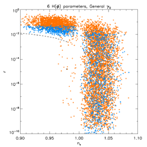
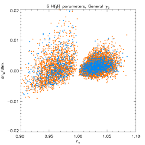
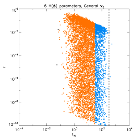
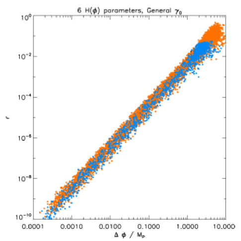
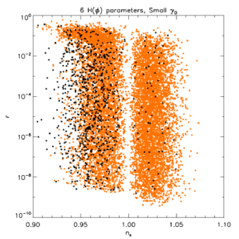
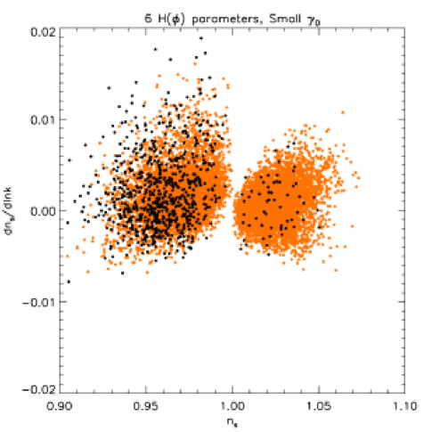
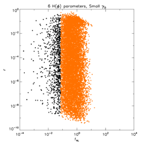
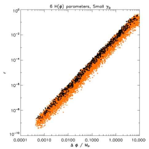
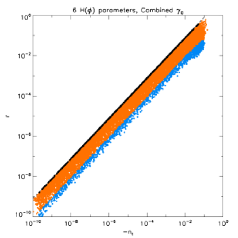
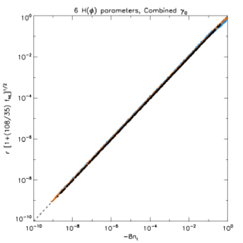
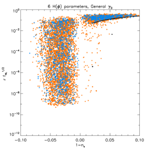
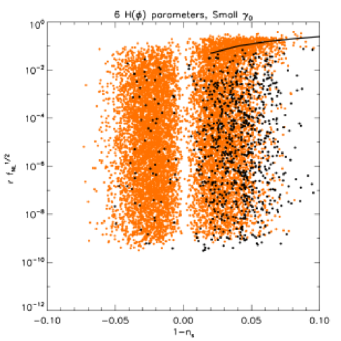
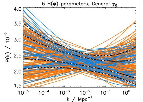
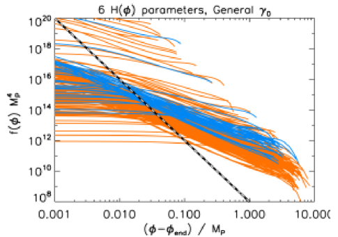
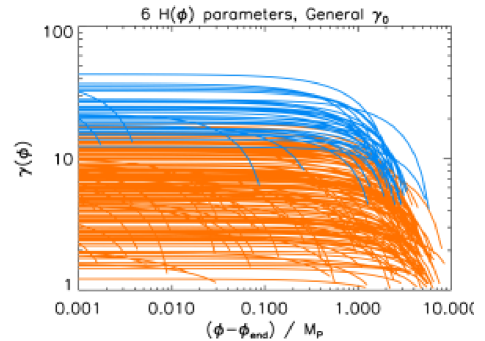
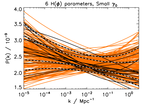
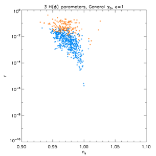
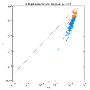
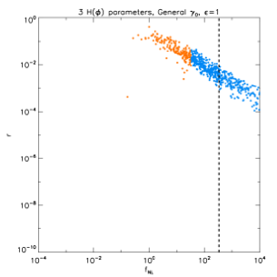
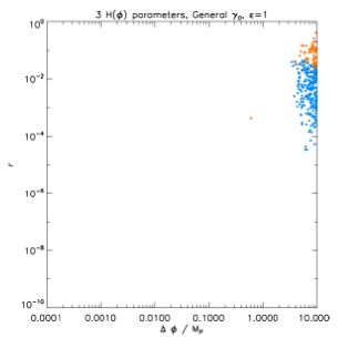
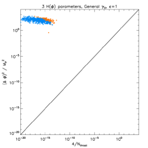
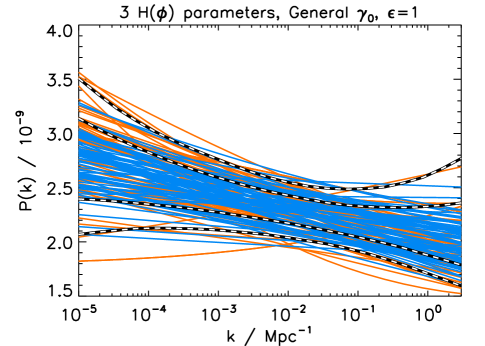
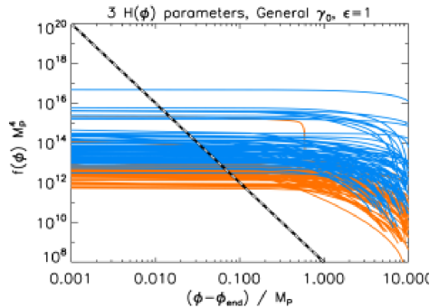
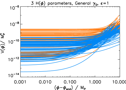
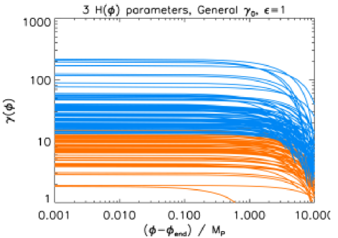
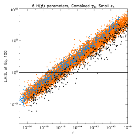
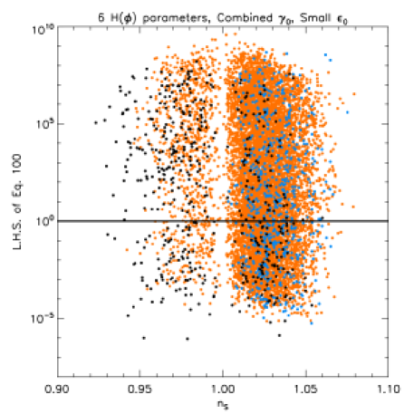
In Figures 1 to 11, we present our results for observables at CMB scales as well as the functions associated with the underlying models. We classify DBI models by their value of at CMB scales: , , define the slow roll (black), intermediate DBI (orange) and ultra-relativistic DBI (blue) regimes, respectively.
Different combinations of the priors on and described in §IV.3 have been applied to each figure. All figures except Fig. 11 use the general prior; the latter has the small prior applied. As specified in the figure captions, sometimes we will show the general and small prior simulations separately to emphasize different points of interest, and sometimes we will combine these simulations. While in general the plots with combined priors have different measures on models in each simulation, this does not matter for our purpose, which is to investigate the functional parameters and predictions of these models qualitatively.
In addition, all figures except Figs. 9 and 10 show simulations run with and in equations (82) and (83); the latter used and . In the case with six parameters, we found that all of the models had inflation ending with tachyonic transitions. This is because models with significant higher order derivatives of which end inflation with have a strong tendency to provide insufficient -folds of inflation to satisfy our requirements, and are therefore rejected from our simulations. In order to get a fraction of models where inflation ended with the end of slow roll, , we had to reduce the number of parameters to three; even in this case, tachyonic transitions were the dominant mechanism for the end of inflation. In Figs. 9 and 10 we show the properties of only the models where inflation ended with .
Here we highlight and comment on what we consider to be the most important results of this study. Further details can be found in the figures and the figure captions.
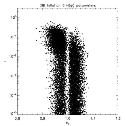
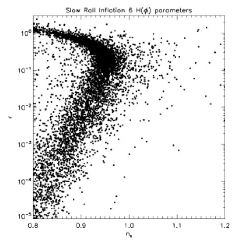
Fig. 1 compares the distributions of points in the vs plane from a Kinney-style single-field slow roll simulation Kinney and a DBI simulation. Note that the algorithm used to create the slow roll simulation is significantly different from ours; among other dissimilarities, it makes use of both forward and backward integration of the single-field slow roll flow equations, while our algorithm only uses forward integration of the generalized flow equations. The slow roll simulation is shown here because it adopts a similar philosophy that “fundamental” quantities of interest which are not strictly fixed by theory, such as the potential, should be Monte-Carlo’d rather than fixed to specific functions when investigating the range of observable properties predicted by a given model. More detailed inferences should not be made from this comparison because of the differences in algorithms.
A paucity of points is apparent in the DBI simulation as . We explain this as follows: For perfect AdS warp factors and a linear Hubble parameter one may show analytically that to all orders in inflationary slow roll parameters Tye . However, it has also been shown that non-linear corrections to and deviations of the warp factors from the AdS limit lead to deviations from scale invariance Shiu . This is what we are seeing here. Our warp factors are generally flatter than AdS for the regime of cosmological interest, and is often non-negligible. Below we explain why we believe our algorithm preferentially selects non-AdS warp factors. The same argument then explains the lack of models leading to perfect scale invariance.
Fig. 2 and 3 present the results for the basic cosmological observables evaluated on CMB scales for general prior and small prior, respectively. As illustrated in Fig. 2(a), which shows vs. , models with detectably large values for the non-Gaussianity parameter satisfy a lower limit on the tensor-to-scalar ratio if the scalar spectrum is red . This bound was derived in Lidsey_Seery ; Lidsey and may be written as
| (98) |
Notice that the bound (98) only applies if , as can be seen from the vs. plot in Fig. 3(a). Since current CMB and large-scale structure data are strongly indicating a red scalar spectrum Observations , Fig. 2 then implies the exciting prediction that DBI models with detectably large non-Gaussianities correlate with detectably large tensors. Unfortunately, this conclusion ignores an important theoretical consistency constraint that should be imposed on any viable model. As Ref. BauMcA showed, the inflation field range in warped D-brane inflation is geometrically limited, and in explicit models can be written in the following simple form
| (99) |
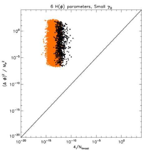
where . By the Lyth bound LythBound this impossibility of super-Planckian field variation during inflation implies a strong upper limit on . For the generalized warp factors studied in this paper the field range bound is written in the generalized form (49). Fig. 5 illustrates this bound for the models shown in Fig. 2 and 3. The plots show rather dramatically that all models in Fig. 2 and 3 violate the microscopic bound of BauMcA .
To find models that satisfy the field range bound (49) we ran separate simulations with small prior. The results are illustrated in Fig. 11. Here, the –axis represents the compactification constraint on the warped throat volume (42) written in the following form
| (100) |
This condition has to be imposed as a consistency constraint on all models. Models that violate (100) correspond to a mismatch between the field range required by the specific inflationary model and the field range allowed by the compactification. We find that (100) can only be satisfied if the field range from IR () to UV () is very small (in Planck units). This is because the magnitude of is constrained to be large by the normalization of the scalar spectrum, so the size of the integral can’t be made small by making small. Instead the integral can only be small if the range of integration is small. By the Lyth bound this small range for the field variation corresponds to a very small tensor signal.
From Fig. 11 we see that theoretically consistent intermediate and ultra-relativistic DBI models satisfy a very strong upper bound on tensors: . This limit is consistent with the bound (98) since the second plot in Fig. 11 shows that all consistent models with large (so that (98) applies) have a blue spectrum . These models could therefore be falsified in the near future if the current indications of a red spectrum gains in statistical significance to be more than .
We emphasize, however, that the bound of is not absolute and in particular does not apply to slow roll models with small . The upper limit on for consistent slow roll models (black points) in Fig. 11 depends on the lower limit of the prior on . For very small , larger becomes consistent with the field range bound. (Similar conclusions were obtained by Bean et al. Bean . In particular, they showed that only extreme slow models with survive the bound of BauMcA ). However, the theoretical considerations of BauMcA still apply, which predict an ultimate upper limit on for slow roll models. This limit is far below the detection sensitivity of any realistic future experiments.
We now comment on the shapes of the empirical derived from our simulations as compared to the analytic AdS warp factor studied in the literature in connection with DBI models. In our simulations with 6 parameters, many of the recovered , as seen in Figs 7(b) and 8(b), exhibit power-law behavior similar to the AdS warp factor, but are somewhat shallower than the AdS case. Further, there are some models which start out with power-law behavior and flatten out towards the end of inflation. In the case of our simulations with 3 parameters, where we consider models where inflation ends with , the derived shapes are exclusively of the latter kind. Our work shows that, qualitatively, there are some differences between the shapes of warp factors found through the empirical process described in our algorithm and the analytical considerations so far. However, given the large parameter space explored in our simulations, there was no a priori expectation that we would recover this particular function. Therefore, it is encouraging that the derived functions are not, in fact, dramatically different from the analytic form. Given that our prior is broad enough to allow warp factors to be generated in a Monte-Carlo fashion, two possibilities are that either the shallower functional forms are more likely to be encountered in the prior, or that the penalty function used in our Metropolis-Hastings algorithm prefers shallower functions over steeper ones. In a future study, we plan to make a full investigation of the likelihood of the analytic AdS warp factor compared to the derived empirical warp factors, in order to test whether the data in fact prefers shallower functions for .
VI Conclusion
In this paper we studied the basic phenomenology of D-brane inflation models with general speed of sound. We developed a general Monte-Carlo formalism for studying models with generalized warp factors and inflaton potentials. Most models show large deviations of the speed of sound from the speed of light resulting in exciting observational signatures. Non-Gaussianities are typically large enough to be observable and the standard slow roll consistency relation is violated at a non-negligible level. However, we also showed that most of these phenomenological models cannot be embedded into a consistent string compactification. In particular, the vast majority of models violates the field range bound of BauMcA . UV models of DBI inflation which obey the field range bound are of two distinct types:555In addition, there is the ’IR model’ ChenIR which requires a separate analysis.
-
1.
Slow roll models with unobservably small .
-
2.
Relativistic DBI models with observable , but blue scalar spectrum, .
Let us therefore imagine that future observations yield a firm measurement of a red scalar spectrum, i.e. a statistically significant detection of after marginalizing over (or detecting) and and the “late-time” cosmological parameters. What would this imply for brane inflation in general and the DBI limit in particular? As indicated above, such an observation of the scalar spectrum would effectively rule out relativistic DBI models, without having to perform any measurements of non-Gaussianities. This illustrates that cosmological observations are quickly becoming precise enough, so that many theoretical ideas are highly constrained. DBI inflation is highly falsifiable and might in fact very soon be ruled out by the data.666To be precise, we emphasize that this statement at present only applies to realizations of the DBI mechanism using D3-branes on Calabi-Yau cones. In this sense our conclusions do not represent model-independent constraints on the DBI mechanism. In particular, all our statements are restricted to the concrete realizations of DBI inflation that we described in §II. Given that the strong constraints on these models are mostly driven by the geometrical field range bound of BauMcA , it would be very interesting to find generalizations of this class of models that evade the bound. Concrete efforts to construct such scenarios are under way DBIv2Eva ; DBIv2SarahLouis . This conclusion motivates considering slow roll models of brane inflation. However, these models suffer from a version of the supergravity eta-problem KKLMMT ; moduli stabilization effects typically induces large corrections to the inflation mass and inflation cannot occur. Given the prospect that relativistic DBI inflation via D3-brane motion on Calabi-Yau cones might soon be ruled out by the data, it becomes important to understand whether the eta-problem for slow roll brane inflation can be overcome BDKM ; Burgess ; Krause .
We are living in the fortunate age where the cosmological data are becoming precise enough to significantly constrain theoretical models of the early universe.
Acknowledgments
We are grateful to Rachel Bean, Igor Klebanov, Liam McAllister, Daniel Mortlock, Sarah Shandera, Eva Silverstein, and Henry Tye for helpful discussions. We thank Richard Easther and Liam McAllister for comments on a draft. HVP is supported by NASA through Hubble Fellowship grant #HF-01177.01-A awarded by the Space Telescope Science Institute, which is operated by the Association of Universities for Research in Astronomy, Inc., for NASA, under contract NAS 5-26555. HVP acknowledges the hospitality of the TAPIR group at Caltech, where part of this work was carried out as a Moore Program visitor. AC acknowledges support from NSF CAREER AST-0645427.
Appendix A Monte-Carlo Algorithm for DBI Inflation
In §IV.3, we gave a broad outline of the Monte-Carlo algorithm that we use to produce the numerical results of §V. In this Appendix, we describe its implementation in detail.
The sign convention is tied as follows to the physical picture of a brane evolving from the UV mouth of the warped throat towards its IR tip. As time increases, the brane falls into the throat towards the end of inflation. We will call this direction forward. as the brane moves forward. at the end of inflation by convention, and large at ; i.e. where . In practice, we set to some large value, and once we find by evolving forward, we just translate the zero point so that .
A.1 Initial Conditions
First, since we define be the UV end of the throat, then by definition,
| (101) |
and
| (102) |
As stated in the main text, we apply several different types of priors on and , as follows:
-
•
General initial conditions: We draw randomly from the broad flat prior .
-
•
Small initial conditions: We draw randomly from the narrow flat prior .
-
•
General initial conditions: We draw randomly from the broad flat prior .
-
•
Small initial conditions: We draw randomly from the narrow flat prior .
The rest of the algorithm is identical for all priors.
We draw the initial amplitude of the power spectrum of scalar density perturbations at and its value at the CMB scale (taken to be Mpc-1) from flat priors,
| (103) |
We select a limited number of the slow variation parameters in equations (82, 83) and Monte-Carlo over their initial conditions using the following flat priors.
| (104) |
Other (higher order) parameters are set to zero at the initial conditions, and therefore remain zero for the entire evolution.
With the choice of parameters in Eq. (104), we have expanded and polynomials to 6th- and 2nd-order in the scalar field , respectively. Such an expansion is more than adequate to capture, for example, the behavior of functions such as through Eq. (65). We have checked that our qualitative results do not change by adding higher order slow evolution parameters to the dynamics.
A.2 Evolution and Matching to CMB Scales
We numerically evolve the flow equations forward into the throat ( decreases) until the matching condition
| (105) |
is satisfied. Then we need to identify the value corresponding to . Note that unlike in slow roll inflation, the horizon exit for scalar and tensor modes for a given physical scale happens at different values, and respectively. These are related by
| (106) |
Rewriting this in a way to minimize numerical errors in the matching,
| (107) | |||||
where is the arbitrary number of -folds associated with .
Models which never satisfy the matching condition (105) are rejected. In addition, throughout the evolution, we impose the following constraints:
-
1.
In order to be compatible with the physical picture of single throat UV DBI inflation, the model must have a monotonically increasing warp factor, i.e. must be satisfied at all times during the evolution.
-
2.
must be a monotonic function. This requires , where
(108) Since , the condition implies
(109) In other words, the sound horizon shouldn’t grow exponentially as the field evolves over Planckian distances.
-
3.
In the single throat scenarios that we are modeling, is constrained to be negative. To see this note that
(110) For a brane moving into a throat is necessarily monotonically increasing, because both and are monotonically increasing as the brane speeds up while moving towards larger warping. With our convention this implies that .
-
4.
, by definition.
-
5.
Successful models must be able to accommodate at least the range of physical scales Mpc-1 between and .
Models failing any one of these requirements are rejected from the simulation.
A.3 End of Inflation
We consider two distinct scenarios for the end of inflation: tachyonic instability and the end of slow roll. In order to capture the uncertainties in the reheating energy scale which translate into significant uncertainties in the number of -folds of inflation between the CMB scale exiting the horizon and the end of inflation Kinney:2005in we draw a random number of -folds to be sampled from . Then we evolve forward towards the end of inflation so that . Defining and computing and , we check that . This is our model for inflation ending via a tachyonic transition. If slow roll ends (i.e. ) before is reached, we identify this as the end of inflation if this occurs at least 40 -folds from the CMB scale, taking the number of -folds between and as . If neither of these conditions are satisfied, the model is rejected.
References
- (1) A. H. Guth, Phys. Rev. D 23, 347 (1981); A. D. Linde, Phys. Lett. B 108, 389 (1982); A. Albrecht and P. J. Steinhardt, Phys. Rev. Lett. 48, 1220 (1982).
- (2) G. R. Dvali and S. H. H. Tye, Phys. Lett. B 450, 72 (1999).
- (3) S. Kachru, R. Kallosh, A. Linde, J. Maldacena, L. McAllister and S. P. Trivedi, JCAP 0310, 013 (2003).
- (4) S. Alexander, Phys. Rev. D 65, 023507 (2002); G. Dvali, Q. Shafi and S. Solganik, [arXiv:hep-th/0105203]; C. P. Burgess, M. Majumdar, D. Nolte, F. Quevedo, G. Rajesh and R. J. Zhang, JHEP 07, 047 (2001); J. H. Brodie and D. A. Easson, JCAP 0312, 004 (2003); K. Becker, M. Becker and A. Krause, Nucl. Phys. B 715, 349 (2005).
- (5) E. Silverstein and D. Tong, Phys. Rev. D 70, 103505 (2004); M. Alishahiha, E. Silverstein and D. Tong, Phys. Rev. D 70, 123505 (2004).
- (6) J. P. Conlon and F. Quevedo, JHEP 0601, 146 (2006); J. R. Bond, L. Kofman, S. Prokushkin and P. M. Vaudrevange, arXiv:hep-th/0612197.
- (7) J. J. Blanco-Pillado et al., JHEP 0609, 002 (2006).
- (8) S. Dimopoulos, S. Kachru, J. McGreevy and J. G. Wacker, arXiv:hep-th/0507205; R. Easther and L. McAllister, JCAP 0605, 018 (2006).
- (9) D. N. Spergel et al. [WMAP Collaboration], Astrophys. J. Suppl. 148, 175 (2003); H. V. Peiris et al., Astrophys. J. Suppl. 148, 213 (2003); D. N. Spergel et al., arXiv:astro-ph/0603449; M. Tegmark et al., Phys. Rev. D 74, 123507 (2006); S. Cole et al. [The 2dFGRS Collaboration], Mon. Not. Roy. Astron. Soc. 362, 505 (2005).
- (10) X. Chen, M. x. Huang, S. Kachru and G. Shiu, JCAP 0701, 002 (2007).
- (11) J. E. Lidsey and D. Seery, Phys. Rev. D 75, 043505 (2007).
- (12) D. Baumann and L. McAllister, Phys. Rev. D 75, 123508 (2007).
- (13) R. Bean, S. E. Shandera, S. H. H. Tye and J. Xu, arXiv:hep-th/0702107.
- (14) J. E. Lidsey and I. Huston, arXiv:0705.0240 [hep-th].
- (15) S. Kachru, R. Kallosh, A. Linde and S. P. Trivedi, Phys. Rev. D 68, 046005 (2003).
- (16) M. R. Douglas and S. Kachru, arXiv:hep-th/0610102.
- (17) S. B. Giddings, S. Kachru and J. Polchinski, Phys. Rev. D 66, 106006 (2002).
- (18) L. Randall and R. Sundrum, Phys. Rev. Lett. 83, 3370 (1999).
- (19) X. Chen, JHEP 0508, 045 (2005) [arXiv:hep-th/0501184]; X. Chen, Phys. Rev. D 72, 123518 (2005) [arXiv:astro-ph/0507053].
- (20) D. Baumann, A. Dymarsky, I. R. Klebanov, J. Maldacena, L. McAllister and A. Murugan, JHEP 0611, 031 (2006).
- (21) S. E. Shandera and S. H. Tye, JCAP 0605, 007 (2006).
- (22) D. Baumann, A. Dymarsky, I. R. Klebanov and L. McAllister, arXiv:0706.0360 [hep-th]; D. Baumann, A. Dymarsky, I. R. Klebanov, L. McAllister, and P. Steinhardt arXiv:0705.3837 [hep-th].
- (23) J. Garriga and V. F. Mukhanov, Phys. Lett. B 458, 219 (1999).
- (24) J. M. Cline, arXiv:hep-th/0612129.
- (25) J. M. Maldacena, JHEP 0305, 013 (2003).
- (26) P. Creminelli, L. Senatore, M. Zaldarriaga and M. Tegmark, JCAP 0703, 005 (2007).
- (27) K. M. Smith and M. Zaldarriaga, arXiv:astro-ph/0612571.
- (28) T. L. Smith, H. V. Peiris and A. Cooray, Phys. Rev. D 73, 123503 (2006).
- (29) I. R. Klebanov and M. J. Strassler, JHEP 0008, 052 (2000).
- (30) D. H. Lyth, Phys. Rev. Lett. 78, 1861 (1997).
- (31) M. B. Hoffman and M. S. Turner, Phys. Rev. D 64, 023506 (2001).
- (32) W. H. Kinney, Phys. Rev. D 66, 083508 (2002).
- (33) R. Easther and W. H. Kinney, Phys. Rev. D 67, 043511 (2003).
- (34) A. R. Liddle, Phys. Rev. D 68, 103504 (2003).
- (35) W. H. Kinney, E. W. Kolb, A. Melchiorri and A. Riotto, Phys. Rev. D 74, 023502 (2006).
- (36) W. H. Kinney, Phys. Rev. D 66, 083508 (2002).
- (37) W. H. Kinney and A. Riotto, JCAP 0603, 011 (2006).
- (38) M. Cortes, A. R. Liddle and P. Mukherjee, arXiv:astro-ph/0702170.
- (39) H. Peiris and R. Easther, JCAP 0610, 017 (2006).
- (40) G. Shiu and B. Underwood, Phys. Rev. Lett. 98, 051301 (2007); S. Kecskemeti, J. Maiden, G. Shiu and B. Underwood, JHEP 0609, 076 (2006).
- (41) G. Hinshaw et al. [WMAP Collaboration], arXiv:astro-ph/0603451.
- (42) L. Page et al. [WMAP Collaboration], arXiv:astro-ph/0603450.
- (43) M. Tegmark et al. [SDSS Collaboration], Astrophys. J. 606, 702 (2004).
- (44) H. Peiris and R. Easther, JCAP 0607, 002 (2006).
- (45) E. Komatsu and D. N. Spergel, Phys. Rev. D 63, 063002 (2001).
- (46) L. Verde, H. Peiris and R. Jimenez, JCAP 0601, 019 (2006).
- (47) M. Kesden, A. Cooray and M. Kamionkowski, Phys. Rev. Lett. 89, 011304 (2002).
- (48) L. Knox and Y. S. Song, Phys. Rev. Lett. 89, 011303 (2002).
- (49) Eva Silverstein, private communication.
- (50) Sarah Shandera and Louis Leblond, private communications.
- (51) C. P. Burgess, J. M. Cline, K. Dasgupta and H. Firouzjahi, arXiv:hep-th/0610320.
- (52) A. Krause and E. Pajer, arXiv:0705.4682 [hep-th].