Fast Adaptive Algorithms in the Non-Standard Form for Multidimensional Problems

Gregory Beylkin, Vani Cheruvu and Fernando Pérez Department of Applied Mathematics, University of Colorado, Boulder, CO 80309-0526, United States
Abstract

We present a fast, adaptive multiresolution algorithm for applying integral operators with a wide class of radially symmetric kernels in dimensions one, two and three. This algorithm is made efficient by the use of separated representations of the kernel. We discuss operators of the class (Δ+μ2I)αsuperscriptΔsuperscript𝜇2𝐼𝛼(-\Delta+\mu^{2}I)^{-\alpha}, where μ0𝜇0\mu\geq 0 and 0<α<3/20𝛼320<\alpha<3/2, and illustrate the algorithm for the Poisson and Schrödinger equations in dimension three. The same algorithm may be used for all operators with radially symmetric kernels approximated as a weighted sum of Gaussians, making it applicable across multiple fields by reusing a single implementation.

This fast algorithm provides controllable accuracy at a reasonable cost, comparable to that of the Fast Multipole Method (FMM). It differs from the FMM by the type of approximation used to represent kernels and has an advantage of being easily extendable to higher dimensions.

keywords:
Separated representation; multiwavelets; adaptive algorithms; integral operators.
thanks: This research was partially supported by DOE grant DE-FG02-03ER25583, DOE/ORNL grant 4000038129 and DARPA/ARO grant W911NF-04-1-0281.

1 Introduction

For a number of years, the Fast Multipole Method (FMM) [1, 2, 3] has been the method of choice for applying integral operators to functions in dimensions d3𝑑3d\leq 3. On the other hand, multiresolution algorithms in wavelet and multiwavelet bases introduced in [4] for the same purpose were not efficient enough to be practical in more than one dimension. Recently, with the introduction of separated representations [5, 6, 7], practical multiresolution algorithms in higher dimensions [8, 9, 10, 11] became available as well. In this paper we present a new fast, adaptive algorithm for applying a class of integral operators with radial kernels in dimensions d=1,2,3𝑑123d=1,2,3, and we briefly discuss its extension to higher dimensions.

In physics, chemistry and other applied fields, many important problems may be formulated using integral equations, typically involving Green’s functions as their kernels. Often such formulations are preferable to those via partial differential equations (PDEs). For example, evaluating the integral expressing the solution of the Poisson equation in free space (the convolution of the Green’s function with the mass or charge density) avoids issues associated with the high condition number of a PDE formulation. Integral operators appear in fields as diverse as electrostatics, quantum chemistry, fluid dynamics and geodesy; in all such applications fast and accurate methods for evaluating operators on functions are needed.

The FMM and our approach both employ approximate representations of operators to yield fast algorithms. The main difference lies in the type of approximations that are used. For example, for the Poisson kernel 1/r1𝑟1/r in dimension d=3𝑑3d=3, the FMM [3] uses a plane wave approximation starting from the integral

1r=12π0eλ(zz0)02πeiλ((xx0)cosα+(yy0)sinα)𝑑α𝑑λ,1𝑟12𝜋superscriptsubscript0superscript𝑒𝜆𝑧subscript𝑧0superscriptsubscript02𝜋superscript𝑒𝑖𝜆𝑥subscript𝑥0𝛼𝑦subscript𝑦0𝛼differential-d𝛼differential-d𝜆\frac{1}{r}=\frac{1}{2\pi}\int_{0}^{\infty}e^{-\lambda(z-z_{0})}\int_{0}^{2\pi}e^{i\lambda((x-x_{0})\cos\alpha+(y-y_{0})\sin\alpha)}d\alpha d\lambda, (1)

where r=(xx0)2+(yy0)2+(zz0)2𝑟superscript𝑥subscript𝑥02superscript𝑦subscript𝑦02superscript𝑧subscript𝑧02r=\sqrt{(x-x_{0})^{2}+(y-y_{0})^{2}+(z-z_{0})^{2}}. The elegant approximation derived from this integral in [3] is valid within a solid angle, and thus requires splitting the application of an operator into directional regions; the number of such regions grows exponentially with dimension. For the same kernel, our approach starts with the integral

1r=2πer2e2s+s𝑑s,1𝑟2𝜋superscriptsubscriptsuperscript𝑒superscript𝑟2superscript𝑒2𝑠𝑠differential-d𝑠\frac{1}{r}=\frac{2}{\sqrt{\pi}}\int_{-\infty}^{\infty}e^{-r^{2}e^{2s}+s}ds, (2)

and its discretization with finite accuracy ϵitalic-ϵ\epsilon yields a spherically symmetric approximation as a weighted sum of gaussians. Other radial kernels can be similarly treated by a suitable choice of integrals. The result is a separated representation of kernels and, therefore, an immediate reduction in the cost of their application. This difference in the choice of approximation dictates the differences in the corresponding algorithms. In dimension d3𝑑3d\leq 3 both approaches are practical and yield comparable performance. The key advantage of our approach is its straightforward extensibility to higher dimensions [6, 7].

Given an arbitrary accuracy ϵitalic-ϵ\epsilon, we effectively represent kernels by a set of exponents and weights describing the terms of the gaussian approximation of integrals like in (2). The number of terms in such sum is roughly proportional to log(ϵ1)superscriptitalic-ϵ1\log(\epsilon^{-1}), or a low power of log(ϵ1)superscriptitalic-ϵ1\log(\epsilon^{-1}), depending on the operator. Since operators are fully described up to an accuracy ϵitalic-ϵ\epsilon by the exponents and weights of the sum of gaussians, a single algorithm applies all such operators. These include operators such as (Δ+μ2I)αsuperscriptΔsuperscript𝜇2𝐼𝛼(-\Delta+\mu^{2}I)^{-\alpha}, where μ0𝜇0\mu\geq 0 and 0<α<3/20𝛼320<\alpha<3/2, and certain singular operators such as the projector on divergence-free functions. Since many physically significant operators depend only on the distance between interacting objects, our approach is directly applicable to problems involving a wide class of operators with radial kernels.

We combine separated and multiresolution representations of kernels and use multiwavelet bases [12] that provide inter alia a method for discretizing integral equations, as is the case in quantum chemistry [8, 9, 11, 10]. This choice of multiresolution bases accommodates integral and differential operators as well as a wide variety of boundary conditions, without degrading the order of the method [13, 14]. Multiwavelet bases retain the key desired properties of wavelet bases, such as vanishing moments, orthogonality, and compact support. Due to the vanishing moments, wide classes of integro-differential operators have an effectively sparse matrix representation, i.e., they differ from a sparse matrix by an operator with small norm. Some of the basis functions of multiwavelet bases are discontinuous, similar to those of the Haar basis and in contrast to wavelets with regularity (see e.g. [15, 16]). The usual choices of scaling functions for multiwavelet bases are either the scaled Legendre or interpolating polynomials. Since these are also used in the discontinuous Galerkin and discontinuous spectral elements methods, our approach may also be seen as an adaptive extension of these methods.

The algorithm for applying an operator to a function starts with computing its adaptive representation in a multiwavelet basis, resulting in a 2dsuperscript2𝑑2^{d}-tree with blocks of coefficients at the leaves. Then the algorithm adaptively applies the (modified) separated non-standard form [4] of the operator to the function by using only the necessary blocks as dictated by the function’s tree representation. We note that in higher dimensions, d3much-greater-than𝑑3d\gg 3, functions need to be in a separated representation as well, since the usual constructions via bases or grids are prohibitive (see [6, 7]).

We start in Section 2 by recalling the basic notions of multiresolution analysis, non-standard operator form and adaptive representation of functions underlying our development. We then consider the separated representation for radially symmetric kernels in Section 3, and use it to efficiently extend the modified ns-form to multiple spatial dimensions in Section 4. We pay particular attention to computing the band structure of the operator based on one dimensional information. We use this construction in Section 5 to introduce the adaptive algorithm for application of multidimensional operators in the modified ns-form, and illustrate its performance in Section 6. We consider two examples: the Poisson equation in free space and the ground state of the Hydrogen atom. We conclude with a brief discussion in Section 7.

2 Preliminary considerations

This section and Appendix are provided for the convenience of the reader in order to keep this paper reasonably self-contained. We provide background material and introduce necessary notation.

The essence of our approach is to decompose the operator using projectors on a Multiresolution Analysis (MRA), and to efficiently apply its projections using a separated representation. We use the decomposition of the operator into the ns-form [4], but we organize it differently (thus, modified ns-form) to achieve greater efficiency. This modification becomes important as we extend this algorithm to higher dimensions.

In this section we introduce notation for MRA, describe the adaptive representation of functions and associated data structures, introduce the modified ns-form and an algorithm for its adaptive application in dimension d=1𝑑1d=1 as background material for the multidimensional case.

2.1 Multiresolution analysis

Let us consider the multiresolution analysis as a decomposition of L2([0,1]d)superscript𝐿2superscript01𝑑L^{2}([0,1]^{d}) into a chain of subspaces

𝐕0𝐕1𝐕2𝐕n,subscript𝐕0subscript𝐕1subscript𝐕2subscript𝐕𝑛\mathbf{V}_{0}\subset\mathbf{V}_{1}\subset\mathbf{V}_{2}\subset\dots\subset\mathbf{V}_{n}\subset\dots,

so that L2([0,1]d)=j=0𝐕j¯superscript𝐿2superscript01𝑑¯superscriptsubscript𝑗0subscript𝐕𝑗L^{2}([0,1]^{d})=\overline{\cup_{j=0}^{\infty}\mathbf{V}_{j}}. We note that our indexing of subspaces (increasing towards finer scales) follows that in [13], and is the reverse of that in [4, 15]. On each subspace 𝐕jsubscript𝐕𝑗\mathbf{V}_{j}, we use the tensor product basis of scaling functions obtained using the functions ϕklj(x)superscriptsubscriptitalic-ϕ𝑘𝑙𝑗𝑥\phi_{kl}^{j}(x) (k=0,,p1)𝑘0𝑝1(k=0,\ldots,p-1) which we briefly describe in Appendix.

The wavelet subspaces 𝐖jsubscript𝐖𝑗\mathbf{W}_{j} are defined as the orthogonal complements of 𝐕jsubscript𝐕𝑗\mathbf{V}_{j} in 𝐕j1subscript𝐕𝑗1\mathbf{V}_{j-1}, thus

𝐕n=𝐕0j=0n𝐖j.subscript𝐕𝑛superscriptsubscriptdirect-sum𝑗0𝑛subscript𝐕0subscript𝐖𝑗\mathbf{V}_{n}=\mathbf{V}_{0}\oplus_{j=0}^{n}\mathbf{W}_{j}\,.

Introducing the orthogonal projector on 𝐕jsubscript𝐕𝑗\mathbf{V}_{j}, 𝐏j:L2([0,1]d)𝐕j:subscript𝐏𝑗superscript𝐿2superscript01𝑑subscript𝐕𝑗\mathbf{P}_{j}:L^{2}([0,1]^{d})\to\mathbf{V}_{j} and considering an operator 𝐓:L2([0,1]d)L2([0,1]d):𝐓superscript𝐿2superscript01𝑑superscript𝐿2superscript01𝑑\mathbf{T}:L^{2}([0,1]^{d})\to L^{2}([0,1]^{d}), we define its projection 𝐓j:𝐕j𝐕j:subscript𝐓𝑗subscript𝐕𝑗subscript𝐕𝑗\mathbf{T}_{j}:\mathbf{V}_{j}\to\mathbf{V}_{j} as 𝐓j=𝐏j𝐓𝐏jsubscript𝐓𝑗subscript𝐏𝑗subscript𝐓𝐏𝑗\mathbf{T}_{j}=\mathbf{P}_{j}\mathbf{T}\mathbf{P}_{j}. We also consider the orthogonal projector 𝐐j:L2([0,1]d)𝐖j:subscript𝐐𝑗superscript𝐿2superscript01𝑑subscript𝐖𝑗\mathbf{Q}_{j}:L^{2}([0,1]^{d})\to\mathbf{W}_{j}, defined as 𝐐j=𝐏j+1𝐏jsubscript𝐐𝑗subscript𝐏𝑗1subscript𝐏𝑗\mathbf{Q}_{j}=\mathbf{P}_{j+1}-\mathbf{P}_{j}.

2.2 Adaptive representation of functions

Let us describe an adaptive refinement strategy for construction multiresolution representations of functions f:BB:𝑓𝐵𝐵f:B\rightarrow B, where B=[0,1]d𝐵superscript01𝑑B=[0,1]^{d}. We proceed by recursive binary subdivision of the box B𝐵B, so the basic structure representing our functions is a 2dlimit-fromsuperscript2𝑑2^{d}-tree with arrays of coefficients stored at the leaves (terminal nodes) and no data stored on internal nodes. On each box obtained via this subdivision, our basis is a tensor product of orthogonal polynomials of degree k=0,,p1𝑘0𝑝1k=0,\ldots,p-1 in each variable, as described in Appendix 8. Therefore, the leaves carry d𝑑d-dimensional arrays of pdsuperscript𝑝𝑑p^{d} coefficients which may be used to approximate function values anywhere in the box corresponding to the spatial region covered by it, via (30) or its equivalent for higher values of d𝑑d. For conciseness, we will often refer to these d𝑑d-dimensional arrays of coefficients stored at tree nodes as function blocks.

This adaptive function decomposition algorithm is similar to that used in [17]. Such construction formally works in any dimension d𝑑d. However, since its complexity scales exponentially with d𝑑d, its practical use is restricted to fairly low dimension, e.g. d4less-than-or-similar-to𝑑4d\lesssim 4. In higher dimensions, alternate representation strategies for functions such as [6, 7] should be considered. In high dimensions, these strategies deal with the exponential growth of complexity by using controlled approximations that have linear cost in d𝑑d.

For simplicity, we will describe the procedure for the one-dimensional case since the extension to dimensions d=2, 3𝑑23d=2,\,3 is straightforward. Since we can not afford to construct our representation by starting from a fine scale (especially in d=3𝑑3d=3), we proceed by successive refinements of an initial coarse sampling. This approach may result in a situation where the initial sampling is insufficient to resolve a rapid change in a small volume; however, in practical applications such situations are rare and may be avoided by an appropriate choice of the initial sampling scale.

Let Blj=[2jl,2j(l+1)]superscriptsubscript𝐵𝑙𝑗superscript2𝑗𝑙superscript2𝑗𝑙1B_{l}^{j}=[2^{-j}l,2^{-j}(l+1)], l=0,,2j1,𝑙0superscript2𝑗1l=0,\ldots,2^{j}-1, represent a binary subinterval on scale j𝑗j. We denote by flj={flj(xk)}k=0p1superscriptsubscript𝑓𝑙𝑗superscriptsubscriptsuperscriptsubscript𝑓𝑙𝑗subscript𝑥𝑘𝑘0𝑝1f_{l}^{j}=\left\{f_{l}^{j}(x_{k})\right\}_{k=0}^{p-1} the vector of values of the function f𝑓f on the Gaussian nodes in Bljsuperscriptsubscript𝐵𝑙𝑗B_{l}^{j}. From these values we compute the coefficients {sklj}k=0p1superscriptsubscriptsuperscriptsubscript𝑠𝑘𝑙𝑗𝑘0𝑝1\left\{s_{kl}^{j}\right\}_{k=0}^{p-1} (see (32) in Appendix) and interpolate f(x)𝑓𝑥f(x) for any xBlj𝑥superscriptsubscript𝐵𝑙𝑗x\in B_{l}^{j} by using (30). We then subdivide Bljsuperscriptsubscript𝐵𝑙𝑗B_{l}^{j} into two child intervals, B2lj+1superscriptsubscript𝐵2𝑙𝑗1B_{2l}^{j+1} and B2l+1j+1superscriptsubscript𝐵2𝑙1𝑗1B_{2l+1}^{j+1}, and evaluate the function f𝑓f on the Gaussian nodes in B2lj+1superscriptsubscript𝐵2𝑙𝑗1B_{2l}^{j+1} and B2l+1j+1superscriptsubscript𝐵2𝑙1𝑗1B_{2l+1}^{j+1}. We then interpolate f𝑓f by using the coefficients {sklj}k=0p1superscriptsubscriptsuperscriptsubscript𝑠𝑘𝑙𝑗𝑘0𝑝1\left\{s_{kl}^{j}\right\}_{k=0}^{p-1} from their parent interval and denote by f~2lj+1superscriptsubscript~𝑓2𝑙𝑗1\widetilde{f}_{2l}^{j+1} and f~2l+1j+1superscriptsubscript~𝑓2𝑙1𝑗1\widetilde{f}_{2l+1}^{j+1} the vectors of interpolated values on the two subintervals. Now, if for a given tolerance ϵitalic-ϵ\epsilon either f2lj+1f~2lj+1>ϵnormsuperscriptsubscript𝑓2𝑙𝑗1superscriptsubscript~𝑓2𝑙𝑗1italic-ϵ\left\|f_{2l}^{j+1}-\widetilde{f}_{2l}^{j+1}\right\|>\epsilon or f2l+1j+1f~2l+1j+1>ϵnormsuperscriptsubscript𝑓2𝑙1𝑗1superscriptsubscript~𝑓2𝑙1𝑗1italic-ϵ\left\|f_{2l+1}^{j+1}-\widetilde{f}_{2l+1}^{j+1}\right\|>\epsilon, we repeat the process recursively for both subintervals, B2lj+1superscriptsubscript𝐵2𝑙𝑗1B_{2l}^{j+1} and B2l+1j+1superscriptsubscript𝐵2𝑙1𝑗1B_{2l+1}^{j+1}; otherwise, we keep the coefficients {sklj}k=0p1superscriptsubscriptsuperscriptsubscript𝑠𝑘𝑙𝑗𝑘0𝑝1\left\{s_{kl}^{j}\right\}_{k=0}^{p-1} to represent the function on the entire interval Bljsuperscriptsubscript𝐵𝑙𝑗B_{l}^{j}. This interval then becomes a leaf in our tree.

At this stage we use the superscript\ell^{\infty} norm, thus constructing an approximation f~~𝑓\tilde{f} to the original function f𝑓f such that ff~<ϵsubscriptnorm𝑓~𝑓italic-ϵ\left\|f-\widetilde{f}\right\|_{\infty}<\epsilon, which immediately implies that ff~2<ϵsubscriptnorm𝑓~𝑓2italic-ϵ\left\|f-\widetilde{f}\right\|_{2}<\epsilon. This estimate clearly extends to any dimension. Once the approximation with superscript\ell^{\infty} norm is constructed, the corresponding tree may be pruned if an application only requires the approximation to be valid in the 2superscript2\ell^{2} norm. We start this process on the finest scale and simply remove all blocks whose cumulative contribution is below ϵitalic-ϵ\epsilon. Other norms, such as H1,subscript𝐻1H_{1}, can be accommodated by appropriately weighing the error tolerance with a scale-dependent factor in the initial (coarse to fine) decomposition process.

The complete decomposition algorithm proceeds by following the above recipe, starting with an initial coarse scale (typically j=0𝑗0j=0) and continuing recursively until the stopping criterion is met for all subintervals. In practice, we choose a stopping scale jmaxsubscript𝑗maxj_{\textrm{max}}, beyond which the algorithm will not attempt to subdivide any further. Reaching jmaxsubscript𝑗maxj_{\textrm{max}} means that the function has significant variations which are not accurately resolved over an interval of width 2jmaxsuperscript2subscript𝑗max2^{-j_{\textrm{max}}} using a basis of order p𝑝p. A pseudo-code listing of this process is presented as Algorithm 1.

Algorithm 1 Adaptive Function Decomposition.
  Start at a coarse scale, typically j=0𝑗0j=0.
  Recursively, for all boxes bjsuperscript𝑏𝑗b^{j} on scale j𝑗j, proceed as follows:
  Construct the list C𝐶C of 2dsuperscript2𝑑2^{d} child boxes bj+1superscript𝑏𝑗1b^{j+1} on scale j+1𝑗1j+1.
  Compute the values of the function f(bj)𝑓superscript𝑏𝑗f(b^{j}) at the pdsuperscript𝑝𝑑p^{d} Gauss-Legendre quadrature nodes in bjsuperscript𝑏𝑗b^{j}.
  for all boxes bj+1Csuperscript𝑏𝑗1𝐶b^{j+1}\in C do
     From f(bj)𝑓superscript𝑏𝑗f(b^{j}), interpolate to the Gauss-Legendre quadrature nodes in bj+1superscript𝑏𝑗1b^{j+1}, producing values f~(bj+1)~𝑓superscript𝑏𝑗1\tilde{f}(b^{j+1}).
     Compute the values of f(bj+1)𝑓superscript𝑏𝑗1f(b^{j+1}) at the Gauss-Legendre nodes of bj+1superscript𝑏𝑗1b^{j+1}, by direct evaluation.
     if f(bj+1)f~(bj+1)>ϵsubscriptnorm𝑓superscript𝑏𝑗1~𝑓superscript𝑏𝑗1italic-ϵ\left\|f(b^{j+1})-\tilde{f}(b^{j+1})\right\|_{\infty}>\epsilon then
        Recursively repeat the entire process for all boxes bj+1Csuperscript𝑏𝑗1𝐶b^{j+1}\in C.
     end if
  end for# Geting here means that the interpolation from the parent was successful for all child boxes. We store the parent’s coefficients from bjsuperscript𝑏𝑗b^{j} in the function tree.

2.2.1 Tree structures for representing functions

The decomposition Algorithm 1 naturally leads to a tree data structure to represent functions, with the leaves of the tree corresponding to the spatial intervals over which the multiwavelet basis provides a sufficiently accurate local approximation. By using (30) or its higher-dimensional extensions, the only data needed to approximate f(x)𝑓𝑥f(x) anywhere in B𝐵B is the array of basis coefficients on these leaves. Thus we use a tree structure where the leaves store these coefficients and the internal nodes do not contain any data (and are effectively removed since we use hash tables for storage). We will refer to this structure as an adaptive tree. Each level in the tree corresponds to a scale in the MRA, with the root node corresponding to the coarsest projection f0𝐕0subscript𝑓0subscript𝐕0f_{0}\in\mathbf{V}_{0}.

Refer to caption
(a) Function.
Refer to caption
(b) Pointwise error.
Refer to caption
(c) Adaptive tree
Refer to caption
(d) Redundant tree
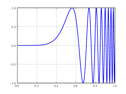
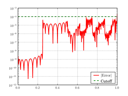
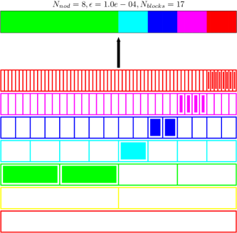
Figure 1: The function f(x)=sin(16πx6)𝑓𝑥16𝜋superscript𝑥6f(x)=\sin(16\pi x^{6}) shown in (a), is decomposed with p=8𝑝8p=8 and ϵ=104italic-ϵsuperscript104\epsilon=10^{-4}; (b) shows the pointwise approximation error. (c) is the resulting adaptive tree, where smaller subdivisions are required in regions with higher frequency content. (d) is the redundant tree associated with this adaptive decomposition, where all internal nodes have been filled with data.

Now, in order to apply the modified non-standard form of an operator to a function, we will show in the next section that we also need the basis coefficients corresponding to internal nodes of the tree. Hence, from the adaptive tree data structure we will compute a similar tree but where we do keep the coefficients of scaling functions on all nodes (leaves and internal).

The coefficients on the internal nodes are redundant since they are computed from the function blocks stored in the leaves. We will thus refer to the tree containing coefficients on all nodes as a redundant tree. It is constructed recursively starting from the leaves, by projecting the scaling coefficients from all sibling nodes onto their parent node, using the decomposition (41).

Figure 1 shows both the adaptive and the redundant trees for a sample function. This figure displays the coarsest scales at the bottom and progressively finer ones further up, with filled boxes representing nodes where scaling coefficients are stored and empty boxes indicating nodes with no data in them (these do not need to be actually stored in the implementation).

2.3 Modified ns-form

The non-standard form [4] (see also [13] for the version specialized for multiwavelets) of the operator 𝐓𝐓\mathbf{T} is the collection of components of the telescopic expansion

𝐓n=(𝐓n𝐓n1)+(𝐓n1𝐓n2)++𝐓0=𝐓0+j=0n1(𝐀j+𝐁j+𝐂j),subscript𝐓𝑛subscript𝐓𝑛subscript𝐓𝑛1subscript𝐓𝑛1subscript𝐓𝑛2subscript𝐓0subscript𝐓0superscriptsubscript𝑗0𝑛1subscript𝐀𝑗subscript𝐁𝑗subscript𝐂𝑗\mathbf{T}_{n}=(\mathbf{T}_{n}-\mathbf{T}_{n-1})+(\mathbf{T}_{n-1}-\mathbf{T}_{n-2})+\dots+\mathbf{T}_{0}=\mathbf{T}_{0}+\sum_{j=0}^{n-1}(\mathbf{A}_{j}+\mathbf{B}_{j}+\mathbf{C}_{j}), (3)

where 𝐀j=𝐐j𝐓𝐐jsubscript𝐀𝑗subscript𝐐𝑗subscript𝐓𝐐𝑗\mathbf{A}_{j}=\mathbf{Q}_{j}\mathbf{T}\mathbf{Q}_{j}, 𝐁j=𝐐j𝐓𝐏jsubscript𝐁𝑗subscript𝐐𝑗subscript𝐓𝐏𝑗\mathbf{B}_{j}=\mathbf{Q}_{j}\mathbf{T}\mathbf{P}_{j}, and 𝐂j=𝐏j𝐓𝐐jsubscript𝐂𝑗subscript𝐏𝑗subscript𝐓𝐐𝑗\mathbf{C}_{j}=\mathbf{P}_{j}\mathbf{T}\mathbf{Q}_{j}. The main property of this expansion is that the rate of decay of the matrix elements of the operators 𝐀jsubscript𝐀𝑗\mathbf{A}_{j}, 𝐁jsubscript𝐁𝑗\mathbf{B}_{j} and 𝐂jsubscript𝐂𝑗\mathbf{C}_{j} away from the diagonal is controlled by the number of vanishing moments of the basis and, for a finite but arbitrary accuracy ϵitalic-ϵ\epsilon, the matrix elements outside a certain band can be set to zero resulting in an error of the norm less than ϵitalic-ϵ\epsilon. Such behavior of the matrix elements becomes clear if we observe that the derivatives of kernels of Calderón-Zygmund and pseudo-differential operators decay faster than the kernel itself. If we use the Taylor expansion of the kernel to estimate the matrix elements away from the diagonal, then the size of these elements is controlled by a high derivative of the kernel since the vanishing moments eliminate the lower order terms [4]. We note that for periodic kernels the band is measured as a periodic distance from the diagonal, resulting in filled-in ‘corners’ of a matrix representation.

Let us introduce notation to show how the telescopic expansion (3) is used when applying an operator to a function. If we apply the projection of the operator 𝐓j1subscript𝐓𝑗1\mathbf{T}_{j-1} not on its “natural scale” j1,𝑗1j-1, but on the finer scale j𝑗j, we denote its upsampled version as (𝐓j1).absentsubscript𝐓𝑗1\uparrow(\mathbf{T}_{j-1}). In the matrix representation of 𝐓j1subscript𝐓𝑗1\mathbf{T}_{j-1}, this operation results in the doubling of the matrix size in each direction. This upsampling ()absent\uparrow(\cdot) and downsampling ()absent\downarrow(\cdot) notation will also be used for projections of functions.

With this notation, computing g=𝐓f𝑔𝐓𝑓g=\mathbf{T}f via (3) splits across scales,

g^0subscript^𝑔0\displaystyle\hat{g}_{0} =\displaystyle= 𝐓0f0subscript𝐓0subscript𝑓0\displaystyle\mathbf{T}_{0}f_{0}
g^1subscript^𝑔1\displaystyle\hat{g}_{1} =\displaystyle= [𝐓1(𝐓0)]f1delimited-[]limit-fromsubscript𝐓1subscript𝐓0subscript𝑓1\displaystyle[\mathbf{T}_{1}-\uparrow(\mathbf{T}_{0})]f_{1}
g^2subscript^𝑔2\displaystyle\hat{g}_{2} =\displaystyle= [𝐓2(𝐓1)]f2delimited-[]limit-fromsubscript𝐓2subscript𝐓1subscript𝑓2\displaystyle[\mathbf{T}_{2}-\uparrow(\mathbf{T}_{1})]f_{2} (4)
\displaystyle\ldots \displaystyle\ldots \displaystyle\ldots
g^jsubscript^𝑔𝑗\displaystyle\hat{g}_{j} =\displaystyle= [𝐓j(𝐓j1)]fjdelimited-[]limit-fromsubscript𝐓𝑗subscript𝐓𝑗1subscript𝑓𝑗\displaystyle[\mathbf{T}_{j}-\uparrow(\mathbf{T}_{j-1})]f_{j}
\displaystyle\ldots \displaystyle\ldots \displaystyle\ldots

where fj=𝐏jfsubscript𝑓𝑗subscript𝐏𝑗𝑓f_{j}=\mathbf{P}_{j}f.

As in the application of the usual ns-form in [4], to obtain gnsubscript𝑔𝑛g_{n} after building the set {g^0,g^1,,g^n},subscript^𝑔0subscript^𝑔1subscript^𝑔𝑛\{\hat{g}_{0},\hat{g}_{1},\ldots,\hat{g}_{n}\}, we have to compute

gn=g^n+(g^n1+(g^n2+(g^n3++(g^0)))).g_{n}=\hat{g}_{n}+\uparrow\left(\hat{g}_{n-1}+\uparrow\left(\hat{g}_{n-2}+\uparrow\left(\hat{g}_{n-3}+\ldots+\left(\uparrow\hat{g}_{0}\right)\ldots\right)\right)\right). (5)

The order of the parentheses in this expression is essential, as it indicates the order of the actual operations which are performed starting on the coarsest subspace 𝐕0.subscript𝐕0\mathbf{V}_{0}. For example, if the number of scales n=4,𝑛4n=4, then (5) yields g4=g^4+(g^3+(g^2+(g^1+(g^0))))subscript𝑔4limit-fromsubscript^𝑔4limit-fromsubscript^𝑔3limit-fromsubscript^𝑔2annotatedlimit-fromsubscript^𝑔1absentsubscript^𝑔0g_{4}=\hat{g}_{4}+\uparrow\left(\hat{g}_{3}+\uparrow\left(\hat{g}_{2}+\uparrow\left(\hat{g}_{1}+\left(\uparrow\hat{g}_{0}\right)\right)\right)\right), describing the sequence of necessary operations.

Unfortunately, the sparsity of the non-standard form induced by the vanishing moments of bases is not sufficient for fast practical algorithms in dimensions other than d=1𝑑1d=1. For algorithms in higher dimensions, we need an additional structure for the remaining non-zero coefficients of the representation. We will use separated representations (see Section 3) introduced in [6, 18] and first applied in a multiresolution setting in [8, 9, 10, 11]. Within the retained bands, the components of the non-standard form are stored and applied in a separated representation and, as a result, the numerical application of operators becomes efficient in higher dimensions.

2.4 Modified ns-form in 1D

Let us describe a one-dimensional construction for operators on L2([0,1])superscript𝐿201L^{2}([0,1]) to introduce all the features necessary for a multidimensional algorithm. Since we use banded versions of operators, we need to introduce the necessary bookkeeping.

The “template” for the band structure on scale j𝑗j comes from the band on the previous scale j1𝑗1j-1. For each block on scale j1𝑗1j-1, the upsampling operation (𝐓j1)absentsubscript𝐓𝑗1\uparrow(\mathbf{T}_{j-1}) creates four blocks (all combinations of even/odd row and column indices). We insist on maintaining the strict correspondence between these four blocks and those of 𝐓jsubscript𝐓𝑗\mathbf{T}_{j}. For this reason the description of the retained blocks of 𝐓jsubscript𝐓𝑗\mathbf{T}_{j} involves the parity of their row and column indices. Let us denote the blocks in the matrix representing 𝐓jsubscript𝐓𝑗\mathbf{T}_{j} by tj;llsuperscript𝑡𝑗𝑙superscript𝑙t^{j;ll^{\prime}}, where l,l=02j1𝑙superscript𝑙0superscript2𝑗1l,l^{\prime}=0\ldots 2^{j-1}. Individual elements within these blocks are indexed as tiij;ll,superscriptsubscript𝑡𝑖superscript𝑖𝑗𝑙superscript𝑙t_{ii^{\prime}}^{j;ll^{\prime}}, where i,i=0,,p1formulae-sequence𝑖superscript𝑖0𝑝1i,i^{\prime}=0,\ldots,p-1, and p𝑝p is the order of the multiwavelet basis. For a given width of the band bj,subscript𝑏𝑗b_{j}, we keep the operator blocks tj;llsuperscript𝑡𝑗𝑙superscript𝑙t^{j;ll^{\prime}} with indices satisfying

lbj+1ll+bj,for even l,lbjll+bj1,for odd l.𝑙subscript𝑏𝑗1absentsuperscript𝑙absent𝑙subscript𝑏𝑗for even l,𝑙subscript𝑏𝑗absentsuperscript𝑙absent𝑙subscript𝑏𝑗1for odd l\begin{array}[]{lrcl}l-b_{j}+1&\leq l^{\prime}\leq&l+b_{j},&\textrm{for even $l$,}\\ l-b_{j}&\leq l^{\prime}\leq&l+b_{j}-1,&\textrm{for odd $l$}.\end{array} (6)

We denote the banded operators where we keep only blocks satisfying (6) as 𝐓jbjsuperscriptsubscript𝐓𝑗subscript𝑏𝑗\mathbf{T}_{j}^{b_{j}} and (𝐓j1)bj.absentsuperscriptsubscript𝐓𝑗1subscript𝑏𝑗\uparrow(\mathbf{T}_{j-1})^{b_{j}}. If we downsample the operator (𝐓j1)bjabsentsuperscriptsubscript𝐓𝑗1subscript𝑏𝑗\uparrow(\mathbf{T}_{j-1})^{b_{j}} back to its original scale j1𝑗1j-1, then (6) leads to the band described by the condition

lbj/2ll+bj/2,𝑙subscript𝑏𝑗2superscript𝑙𝑙subscript𝑏𝑗2l-\left\lfloor b_{j}/2\right\rfloor\leq l^{\prime}\leq l+\left\lfloor b_{j}/2\right\rfloor, (7)

where bj/2subscript𝑏𝑗2\left\lfloor b_{j}/2\right\rfloor denotes the integer part of bj/2.subscript𝑏𝑗2b_{j}/2. We denote the banded operator on scale j1𝑗1j-1 as 𝐓j1bj/2superscriptsubscript𝐓𝑗1subscript𝑏𝑗2\mathbf{T}_{j-1}^{\left\lfloor b_{j}/2\right\rfloor}, where we retain blocks satisfying (7).

If we now rewrite (4) keeping only blocks within the bands on each scale, we obtain

g^0subscript^𝑔0\displaystyle\hat{g}_{0} =\displaystyle= 𝐓0f0subscript𝐓0subscript𝑓0\displaystyle\mathbf{T}_{0}f_{0}
g^1subscript^𝑔1\displaystyle\hat{g}_{1} =\displaystyle= [𝐓1b1(𝐓0)b1]f1=𝐓1b1f1(𝐓0)b1f1delimited-[]limit-fromsuperscriptsubscript𝐓1subscript𝑏1superscriptsubscript𝐓0subscript𝑏1subscript𝑓1limit-fromsuperscriptsubscript𝐓1subscript𝑏1subscript𝑓1superscriptsubscript𝐓0subscript𝑏1subscript𝑓1\displaystyle[\mathbf{T}_{1}^{b_{1}}-\uparrow(\mathbf{T}_{0})^{b_{1}}]f_{1}=\mathbf{T}_{1}^{b_{1}}f_{1}-\uparrow(\mathbf{T}_{0})^{b_{1}}f_{1}
g^2subscript^𝑔2\displaystyle\hat{g}_{2} =\displaystyle= [𝐓2b2(𝐓1)b2]f2=𝐓2b2f2(𝐓1)b2f2delimited-[]limit-fromsuperscriptsubscript𝐓2subscript𝑏2superscriptsubscript𝐓1subscript𝑏2subscript𝑓2limit-fromsuperscriptsubscript𝐓2subscript𝑏2subscript𝑓2superscriptsubscript𝐓1subscript𝑏2subscript𝑓2\displaystyle[\mathbf{T}_{2}^{b_{2}}-\uparrow(\mathbf{T}_{1})^{b_{2}}]f_{2}=\mathbf{T}_{2}^{b_{2}}f_{2}-\uparrow(\mathbf{T}_{1})^{b_{2}}f_{2} (8)
\displaystyle\ldots \displaystyle\ldots \displaystyle\ldots
g^jsubscript^𝑔𝑗\displaystyle\hat{g}_{j} =\displaystyle= [𝐓jbj(𝐓j1)bj]fj=𝐓jbjfj(𝐓j1)bjfjdelimited-[]limit-fromsuperscriptsubscript𝐓𝑗subscript𝑏𝑗superscriptsubscript𝐓𝑗1subscript𝑏𝑗subscript𝑓𝑗limit-fromsuperscriptsubscript𝐓𝑗subscript𝑏𝑗subscript𝑓𝑗superscriptsubscript𝐓𝑗1subscript𝑏𝑗subscript𝑓𝑗\displaystyle[\mathbf{T}_{j}^{b_{j}}-\uparrow(\mathbf{T}_{j-1})^{b_{j}}]f_{j}=\mathbf{T}_{j}^{b_{j}}f_{j}-\uparrow(\mathbf{T}_{j-1})^{b_{j}}f_{j}
\displaystyle\ldots \displaystyle\ldots \displaystyle\ldots

For any arbitrary but finite accuracy, instead of applying the full [𝐓j(𝐓j1)],delimited-[]limit-fromsubscript𝐓𝑗subscript𝐓𝑗1[\mathbf{T}_{j}-\uparrow(\mathbf{T}_{j-1})], we will only apply its banded approximation.

A simple but important observation is that

([(𝐓j1)]fj)=𝐓j1fj1,\downarrow([\uparrow(\mathbf{T}_{j-1})]f_{j})=\mathbf{T}_{j-1}f_{j-1}\,, (9)

which follows from the fact that 𝐐j𝐏j=𝐏j𝐐j=0,subscript𝐐𝑗subscript𝐏𝑗subscript𝐏𝑗subscript𝐐𝑗0\mathbf{Q}_{j}\mathbf{P}_{j}=\mathbf{P}_{j}\mathbf{Q}_{j}=0, since these are orthogonal projections. Thus, we observe that ((𝐓j1)bj)=𝐓j1bj/2;\downarrow(\uparrow(\mathbf{T}_{j-1})^{b_{j}})=\mathbf{T}_{j-1}^{\left\lfloor b_{j}/2\right\rfloor}; so instead of applying (𝐓j1)bjfjabsentsuperscriptsubscript𝐓𝑗1subscript𝑏𝑗subscript𝑓𝑗\uparrow(\mathbf{T}_{j-1})^{b_{j}}f_{j} on scale j𝑗j, we can obtain the same result using (9), so that (𝐓j1bj/2fj1)=(𝐓j1)bjfj\uparrow\left(\mathbf{T}_{j-1}^{\left\lfloor b_{j}/2\right\rfloor}f_{j-1}\right)=\uparrow(\mathbf{T}_{j-1})^{b_{j}}f_{j}. Therefore, we will compute only 𝐓j1bj/2fj1superscriptsubscript𝐓𝑗1subscript𝑏𝑗2subscript𝑓𝑗1\mathbf{T}_{j-1}^{\left\lfloor b_{j}/2\right\rfloor}f_{j-1} on scale j1𝑗1j-1 and combine it with computing 𝐓j1bj1fj1superscriptsubscript𝐓𝑗1subscript𝑏𝑗1subscript𝑓𝑗1\mathbf{T}_{j-1}^{b_{j-1}}f_{j-1}. Incorporating this into (5), we arrive at

gnsubscript𝑔𝑛\displaystyle g_{n} =\displaystyle= 𝐓nbnfn+[(𝐓n1bn1𝐓n1bn/2)fn1+\displaystyle\mathbf{T}_{n}^{b_{n}}f_{n}+\uparrow\left[\left(\mathbf{T}_{n-1}^{b_{n-1}}-\mathbf{T}_{n-1}^{\left\lfloor b_{n}/2\right\rfloor}\right)f_{n-1}+\right.
[(𝐓n2bn2𝐓n2bn1/2)fn2++[[(𝐓0𝐓0b1/2)f0]]]].\displaystyle\left.\left.\uparrow\left[\left(\mathbf{T}_{n-2}^{b_{n-2}}-\mathbf{T}_{n-2}^{\left\lfloor b_{n-1}/2\right\rfloor}\right)f_{n-2}+\ldots+\left[\uparrow\left[\left(\mathbf{T}_{0}-\mathbf{T}_{0}^{\left\lfloor b_{1}/2\right\rfloor}\right)f_{0}\right]\right]\ldots\right.\right]\right].

Using this expression yields an efficient algorithm for applying an operator, as on each scale j𝑗j, 𝐓jbj𝐓j[bj+1/2]superscriptsubscript𝐓𝑗subscript𝑏𝑗superscriptsubscript𝐓𝑗delimited-[]subscript𝑏𝑗12\mathbf{T}_{j}^{b_{j}}-\mathbf{T}_{j}^{[b_{j+1}/2]} is a sparse object, due to the cancellation which occurs for most of the blocks. In particular, 𝐓jbj𝐓j[bj+1/2]superscriptsubscript𝐓𝑗subscript𝑏𝑗superscriptsubscript𝐓𝑗delimited-[]subscript𝑏𝑗12\mathbf{T}_{j}^{b_{j}}-\mathbf{T}_{j}^{[b_{j+1}/2]} is missing the blocks near the diagonal, and we will refer to it as an outer band matrix. We will call 𝐓jbjsuperscriptsubscript𝐓𝑗subscript𝑏𝑗\mathbf{T}_{j}^{b_{j}} a whole band matrix as it contains both the inner and outer bands.
Refer to caption
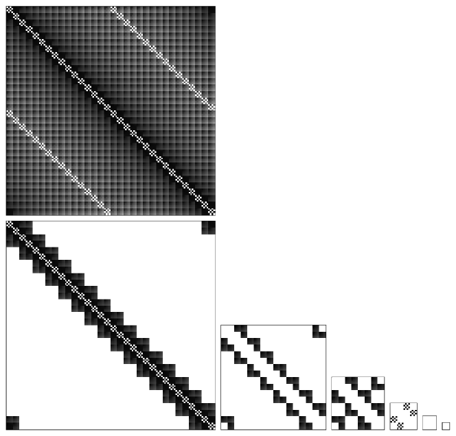
Figure 2: Modified non-standard form of the convolution operator in (11) in a multiwavelet basis, with white representing 0 and black representing large values. The top matrix is the projection of this operator on 𝐕5subscript𝐕5\mathbf{V}_{5}, resulting in a dense matrix. The lower half depicts the multiresolution representation in (2.4) with only the blocks that are actually retained for a given accuracy. We will call the leftmost matrix in this series a whole band matrix and all others outer band matrices. The two empty outer band matrices on scales j=0,1𝑗01j=0,1 are explained in the main text.

The structure of these matrices is illustrated in Figure 2. The two empty scales j=0,1𝑗01j=0,1 arise due to the complete cancellation of blocks on these scales. We note that the modified non-standard form is constructed adaptively in the number of scales necessary for a given function. For just two scales, this construction will have the scale j=1𝑗1j=1 non-empty. Given an adaptive decomposition of a function on n𝑛n scales, we precompute the modified non-standard form (depicted in Figure 2 for five scales) on all scales n,n1,,1𝑛𝑛11n,n-1,\dots,1. For matrices requiring 2n2nsuperscript2𝑛superscript2𝑛2^{n}\cdot 2^{n} blocks on the finest scale n𝑛n, we need to keep and apply only 𝒪(2n)𝒪superscript2𝑛\mathcal{O}(2^{n}) blocks, as with the original non-standard form in [4].

2.4.1 Adaptive application

Let us show how to use the multiscale representation in (2.4) to apply the operator T𝑇T to a function f𝑓f with controlled accuracy ϵitalic-ϵ\epsilon. We describe an adaptive application of the operator to a function, where we assume (as is often the case) that the tree structure of the input is sufficient to adequately describe the output with accuracy ϵitalic-ϵ\epsilon. This assumption will be removed later.

Our algorithm uses the structure shown in Figure 2 in an adaptive fashion. We copy the structure of the redundant tree for the input function, and use that as a template to be filled for the output g𝑔g. For each node of the output tree we determine whether it is a leaf or an internal node: for leaves, we must apply a whole band matrix on the scale of that node, such as the leftmost matrix for j=5𝑗5j=5 in the example shown in Figure 2. For internal nodes, we apply an outer band matrix (for that scale). We note that our construction of the operator produces both whole and outer band matrices for all scales, and we simply choose the appropriate kind for each node of output as needed. Upon completion of this process, we apply the projection (5) to construct the final adaptive tree representing the output.

Algorithm 2 Adaptive non-standard form operator application in d=1𝑑1d=1, g=𝐓f𝑔𝐓𝑓g=\mathbf{T}f
  Initialization: Construct the redundant tree for f𝑓f and copy it as skeleton tree for g𝑔g (see Section 2.2.1).
  for all scales j=0,,n1𝑗0𝑛1j=0,\ldots,n-1 do
     for all function blocks gljsuperscriptsubscript𝑔𝑙𝑗g_{l}^{j} in the tree for g𝑔g at scale j𝑗j do
        # Step 1. Determine the list of all contributing blocks of the modified ns-form 𝐓lljsuperscriptsubscript𝐓𝑙superscript𝑙𝑗{\mathbf{T}_{ll^{\prime}}^{j}} (see Section 2.3):
        if gljsuperscriptsubscript𝑔𝑙𝑗g_{l}^{j} belongs to a leaf then
           Read operator blocks 𝐓lljsuperscriptsubscript𝐓𝑙superscript𝑙𝑗{\mathbf{T}_{ll^{\prime}}^{j}} from row l𝑙l of whole band matrix 𝐓jbjsuperscriptsubscript𝐓𝑗subscript𝑏𝑗\mathbf{T}_{j}^{b_{j}}.
        else
           Read operator blocks 𝐓lljsuperscriptsubscript𝐓𝑙superscript𝑙𝑗{\mathbf{T}_{ll^{\prime}}^{j}} from row l𝑙l of outer band matrix 𝐓jbj𝐓j[bj+1/2]superscriptsubscript𝐓𝑗subscript𝑏𝑗superscriptsubscript𝐓𝑗delimited-[]subscript𝑏𝑗12\mathbf{T}_{j}^{b_{j}}-\mathbf{T}_{j}^{[b_{j+1}/2]}.
        end if
        # Step 2. Find the required blocks fljsuperscriptsubscript𝑓superscript𝑙𝑗{f_{l^{\prime}}^{j}} of the input function f𝑓f:
        if function block fljsuperscriptsubscript𝑓superscript𝑙𝑗{f_{l^{\prime}}^{j}} exists in the redundant tree for f𝑓f then
           Retrieve it.
        else
           Create it by interpolating from a coarser scale and cache for reuse.
        end if
        # Step 3. Output function block computation:
        Compute the resulting output function block according to g^lj=l𝐓lljfljsuperscriptsubscript^𝑔𝑙𝑗subscriptsuperscript𝑙superscriptsubscript𝐓𝑙superscript𝑙𝑗superscriptsubscript𝑓superscript𝑙𝑗\hat{g}_{l}^{j}=\sum_{l^{\prime}}\mathbf{T}_{ll^{\prime}}^{j}f_{l^{\prime}}^{j}, where the operation 𝐓lljfljsuperscriptsubscript𝐓𝑙superscript𝑙𝑗superscriptsubscript𝑓superscript𝑙𝑗\mathbf{T}_{ll^{\prime}}^{j}f_{l^{\prime}}^{j} indicates a regular matrix-vector multiplication.
     end for
  end for
  # Step 4. Adaptive projection:
  Project resulting output function blocks g^ljsuperscriptsubscript^𝑔𝑙𝑗\hat{g}_{l}^{j} on all scales into a proper adaptive tree by using Eq. (5).
  Discard from the resulting tree unnecessary function blocks at the requested accuracy.
  Return: the function g𝑔g represented by its adaptive tree.

Algorithm 2 returns an adaptive tree representing the function g𝑔g. This tree contains sufficient information to evaluate g𝑔g at arbitrary points by interpolation and may be used as an input in further computations.

We note that Step 2 in Algorithm 2 naturally resolves the problem that is usually addressed by mortar methods, see e.g. [19, 20, 21, 22]. Since adaptive representations have neighboring blocks of different sizes, they encounter difficulties when applying non-diagonal operators, as they require blocks which do not exist on that scale. Our approach simply constructs these as needed and caches them for reuse, without requiring any additional consideration on the part of the user.

2.4.2 Numerical example

Let us briefly illustrate the application of the modified ns-form with an example of a singular convolution on the unit circle, the operator with the kernel K(x)=cot(πx),𝐾𝑥𝜋𝑥K(x)=\cot(\pi x),

(Cf)(y)=p.v.01cot(π(yx))f(x)𝑑x,𝐶𝑓𝑦p.v.superscriptsubscript01𝜋𝑦𝑥𝑓𝑥differential-d𝑥(Cf)(y)\,=\mbox{p.v.}\,\int_{0}^{1}\cot(\pi(y-x))\,f(x)\,dx, (11)

a periodic analogue of the Hilbert transform. In order to find its representation in multiwavelet bases, we compute

riij;l= 2j11K(2j(x+l))Φii(x)𝑑x=2j11cot(π 2j(x+l))Φii(x)𝑑x,superscriptsubscript𝑟𝑖superscript𝑖𝑗𝑙superscript2𝑗superscriptsubscript11𝐾superscript2𝑗𝑥𝑙subscriptΦ𝑖superscript𝑖𝑥differential-d𝑥superscript2𝑗superscriptsubscript11𝜋superscript2𝑗𝑥𝑙subscriptΦ𝑖superscript𝑖𝑥differential-d𝑥r_{{ii^{\prime}}}^{j;\,l}\,=\,2^{-j}\,\int_{-1}^{1}\,K(2^{-j}(x+l))\,\Phi_{ii^{\prime}}(x)\,dx\,=2^{-j}\,\int_{-1}^{1}\,\cot(\pi\,2^{-j}(x+l))\,\Phi_{ii^{\prime}}(x)\,dx\,, (12)

where Φii(x)subscriptΦ𝑖superscript𝑖𝑥\Phi_{ii^{\prime}}(x), i,i=0,,k1formulae-sequence𝑖superscript𝑖0𝑘1i,i^{\prime}=0,\ldots,k-1 are cross-correlation functions described in Appendix 8.4 and l=0,±1,±2,2j1𝑙0plus-or-minus1plus-or-minus2superscript2𝑗1l=0,\pm 1,\pm 2,\ldots 2^{j}-1. We compute riij;lsuperscriptsubscript𝑟𝑖superscript𝑖𝑗𝑙r_{{ii^{\prime}}}^{j;\,l} using the convergent integrals

riij;l= 2jk=iii+iciik01Φk,0+(x)(cot(π 2j(x+l))+(1)i+icot(π 2j(x+l)))𝑑x,superscriptsubscript𝑟𝑖superscript𝑖𝑗𝑙superscript2𝑗superscriptsubscript𝑘superscript𝑖𝑖superscript𝑖𝑖superscriptsubscript𝑐𝑖superscript𝑖𝑘superscriptsubscript01superscriptsubscriptΦ𝑘0𝑥𝜋superscript2𝑗𝑥𝑙superscript1𝑖superscript𝑖𝜋superscript2𝑗𝑥𝑙differential-d𝑥r_{{ii^{\prime}}}^{j;\,l}\,=\,2^{-j}\,\sum_{k=i^{\prime}-i}^{i^{\prime}+i}\,c_{ii^{\prime}}^{k}\,\int_{0}^{1}\,\Phi_{k,0}^{+}(x)\,\left(\cot(\pi\,2^{-j}(x+l))+(-1)^{i+i^{\prime}}\cot(\pi\,2^{-j}(-x+l))\right)\,dx,

where Φk,0+superscriptsubscriptΦ𝑘0\Phi_{k,0}^{+} is a polynomial described in Appendix 8.4. In our numerical experiment, we apply (11) to the periodic function on [0,1]01[0,1],

f(x)=kea(x+k1/2)2,𝑓𝑥subscript𝑘superscript𝑒𝑎superscript𝑥𝑘122f(x)=\sum_{k\in\mathbb{Z}}e^{-a(x+k-1/2)^{2}},

which yields

(Cf)(y)=kea(y+k1/2)2Erfi[a(y+k1/2)]=iπansign(n)en2π2/ae2πiny,𝐶𝑓𝑦subscript𝑘superscript𝑒𝑎superscript𝑦𝑘122Erfidelimited-[]𝑎𝑦𝑘12𝑖𝜋𝑎subscript𝑛sign𝑛superscript𝑒superscript𝑛2superscript𝜋2𝑎superscript𝑒2𝜋𝑖𝑛𝑦(Cf)(y)=-\sum_{k\in\mathbb{Z}}e^{-a(y+k-1/2)^{2}}\mbox{Erfi}[\sqrt{a}(y+k-1/2)]=i\sqrt{\frac{\pi}{a}}\sum_{n\in\mathbb{Z}}\mbox{sign}(n)e^{-n^{2}\pi^{2}/a}e^{2\pi iny}, (13)

where ey2Erfi(y)=2π0yes2y2𝑑s.superscript𝑒superscript𝑦2Erfi𝑦2𝜋superscriptsubscript0𝑦superscript𝑒superscript𝑠2superscript𝑦2differential-d𝑠e^{-y^{2}}\mbox{Erfi}(y)=\frac{2}{\sqrt{\pi}}\int_{0}^{y}e^{s^{2}-y^{2}}ds. Expression (13) is obtained by first observing that the Hilbert transform of eax2superscript𝑒𝑎superscript𝑥2e^{-ax^{2}} is eay2Erfi(ay)superscript𝑒𝑎superscript𝑦2Erfi𝑎𝑦-e^{-ay^{2}}\mbox{Erfi}(\sqrt{a}y), and then evaluating the lattice sum, noting that (see [23, formula 4.3.91])

cot(πx)=1π(1x+k=12xx2k2).𝜋𝑥1𝜋1𝑥superscriptsubscript𝑘12𝑥superscript𝑥2superscript𝑘2\cot(\pi x)=\frac{1}{\pi}(\frac{1}{x}+\sum_{k=1}^{\infty}\frac{2x}{x^{2}-k^{2}}).

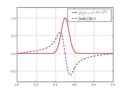
Table 1 summarizes the numerical construction of this solution for a=300𝑎300a=300, at various requested precisions. Optimal performance is obtained by adjusting the order of the basis p𝑝p as a function of the requested precision, to ensure that the operator remains a banded matrix with small band, and that the adaptive representation of the input function requires a moderate number of scales. The resulting numerical error (as compared to the exact analytical solution), measured in the 2superscript2\ell^{2} norm, is shown in the last column. Figure 3 shows the input and results for this example, as well as the point-wise error for the case where ϵreq =1012subscriptitalic-ϵreq superscript1012\epsilon_{\textrm{req }}=10^{-12} and p=14𝑝14p=14 (the last row in the table).

p𝑝p Scales Nblockssubscript𝑁blocksN_{\textrm{blocks}} ϵitalic-ϵ\epsilon E2subscript𝐸2E_{2}
5 [2,3,4] 8 103superscript10310^{-3} 1.51041.5superscript1041.5\cdot 10^{-4}
8 [2,4,5] 12 106superscript10610^{-6} 1.31071.3superscript1071.3\cdot 10^{-7}
11 [2,4,5] 14 109superscript10910^{-9} 1.110101.1superscript10101.1\cdot 10^{-10}
14 [3,4,5] 16 1012superscript101210^{-12} 4.410134.4superscript10134.4\cdot 10^{-13}

Table 1: Results from evaluating (13) with our algorithm. The order of the basis p𝑝p is adjusted as a function of the requested precision ϵitalic-ϵ\epsilon. The second column indicates scales present in the adaptive tree for the input. The third column shows the total number of blocks of coefficients in this tree. The last column (E2subscript𝐸2E_{2}) shows the actual error of the computed solution in the 2superscript2\ell^{2} norm.
Refer to caption
Refer to caption
Figure 3: Results of applying the cotangent kernel to a periodized Gaussian using basis of order p=14𝑝14p=14 (the last row in Table 1). The pointwise error is shown on the right for a requested accuracy of ϵ=1012italic-ϵsuperscript1012\epsilon=10^{-12}.

3 Separated representations of integral kernels

The approach we’ve discussed so far does not efficiently generalize to the application of non-separable multidimensional integral kernels. Since several physically important kernels belong to this category (e.g. the Poisson kernels in d=2𝑑2d=2 and d𝑑d=3), additional tools are needed. We now describe the key idea that allows us to perform this generalization to d>1𝑑1d>1.

We use the separated representation of operators introduced in [6, 24] to reduce the computational cost of the straightforward generalization of the multiresolution approach in [4]. Such representations are particularly simple for convolution operators and are based on approximating kernels by a sum of Gaussians [24, 8, 9, 11, 10]. This approximation has a multiresolution character by itself and requires a remarkably small number of terms. In fact, our algorithm uses the coefficients and the exponents of the Gaussian terms as the only input from which it selects the necessary terms, scale by scale, according the desired accuracy threshold ϵitalic-ϵ\epsilon. Therefore, our algorithm works for all operators with kernels that admit approximation by a sum of Gaussians. Examples of such operators include the Poisson and the bound state Helmholtz Green’s functions, the projector on divergence free functions, as well as regular and fractional derivative operators. Let us consider a particular family of operators (Δ+μ2I)αsuperscriptΔsuperscript𝜇2𝐼𝛼(-\Delta+\mu^{2}I)^{-\alpha}, where μ0𝜇0\mu\geq 0 and 0<α<3/20𝛼320<\alpha<3/2. The kernel of this operator

Kμ,α(r)=232+αCα(μr)32αK32α(μr),subscript𝐾𝜇𝛼𝑟superscript232𝛼subscript𝐶𝛼superscript𝜇𝑟32𝛼subscriptK32𝛼𝜇𝑟K_{\mu,\alpha}(r)=2^{-\frac{3}{2}+\alpha}\cdot C_{\alpha}\cdot(\frac{\mu}{r})^{\frac{3}{2}-\alpha}\textrm{K}_{\frac{3}{2}-\alpha}(\mu r),

where K32αsubscriptK32𝛼\textrm{K}_{\frac{3}{2}-\alpha} is the modified Bessel function, r=𝐱𝐲𝑟norm𝐱𝐲r=||\mathbf{x}-\mathbf{y}|| and Cα=2 22απ32/Γ(α)subscript𝐶𝛼2superscript22𝛼superscript𝜋32Γ𝛼C_{\alpha}=2\cdot\,2^{-2\alpha}\pi^{-\frac{3}{2}}/\Gamma(\alpha), has an integral representation

Kμ,α(r)=Cαer2e2se14μ2e2s+(32α)s𝑑s.subscript𝐾𝜇𝛼𝑟subscript𝐶𝛼superscriptsubscriptsuperscript𝑒superscript𝑟2superscript𝑒2𝑠superscript𝑒14superscript𝜇2superscript𝑒2𝑠32𝛼𝑠differential-d𝑠K_{\mu,\alpha}(r)=C_{\alpha}\,\int_{-\infty}^{\infty}e^{-r^{2}e^{2s}}e^{-\frac{1}{4}\mu^{2}e^{-2s}+(3-2\alpha)s}ds. (14)

Using the trapezoidal rule, we construct an approximation valid over a range of values δrR𝛿𝑟𝑅\delta\leq r\leq R with accuracy ϵitalic-ϵ\epsilon, of the form

|Kμ,α(r)m=1Mwmeτmr2|ϵK0,α(r)=ϵΓ(3/2α)Cα2r32α,subscript𝐾𝜇𝛼𝑟superscriptsubscript𝑚1𝑀subscript𝑤𝑚superscript𝑒subscript𝜏𝑚superscript𝑟2italic-ϵsubscript𝐾0𝛼𝑟italic-ϵΓ32𝛼subscript𝐶𝛼2superscript𝑟32𝛼\left|K_{\mu,\alpha}(r)-\sum_{m=1}^{M}w_{m}e^{-\tau_{m}r^{2}}\right|\leq\epsilon K_{0,\alpha}(r)=\epsilon\frac{\Gamma(3/2-\alpha)\cdot C_{\alpha}}{2r^{3-2\alpha}}, (15)

where τm=e2smsubscript𝜏𝑚superscript𝑒2subscript𝑠𝑚\tau_{m}=e^{2s_{m}}, wm=hCαeμ2e2sm/4+(32α)smsubscript𝑤𝑚subscript𝐶𝛼superscript𝑒superscript𝜇2superscript𝑒2subscript𝑠𝑚432𝛼subscript𝑠𝑚w_{m}=h\,C_{\alpha}\,e^{-\mu^{2}e^{-2s_{m}}/4+(3-2\alpha)s_{m}}, h=(BA)/M𝐵𝐴𝑀h=(B-A)/M and sm=A+mhsubscript𝑠𝑚𝐴𝑚s_{m}=A+mh. The limits of integration, A𝐴A, B𝐵B and the step size hh are selected as indicated in [24], where it is shown that for a fixed accuracy ϵitalic-ϵ\epsilon the number of terms M𝑀M in (15) is proportional to log(Rδ1)𝑅superscript𝛿1\log(R\delta^{-1}). Although it is possible to select δ𝛿\delta and R𝑅R following the estimates in [25] and optimize the number of terms for a desired accuracy ϵitalic-ϵ\epsilon, in this paper we start with an approximation that has an obviously excessive range of validity and thus, an excessive number of terms.

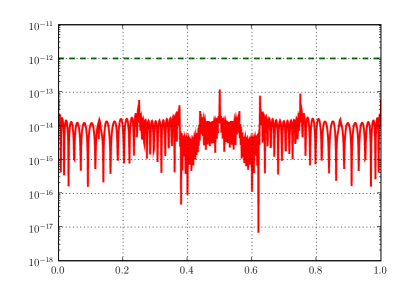
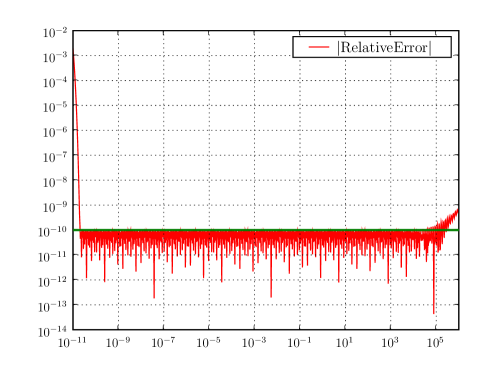
An example of such approximation is shown in Figure 4. For a requested tolerance of ϵ=1010italic-ϵsuperscript1010\epsilon=10^{-10}, roughly 300 terms are enough to provide a valid approximation over a range of 151515 decades. We then let the algorithm choose the necessary terms, scale by scale, to satisfy the user-supplied accuracy requirement ϵitalic-ϵ\epsilon. This approach may end up with a few extra terms on some scales in comparison with that using a nearly optimal number of terms [8, 10, 11, 9]. Whereas the cost of applying a few extra terms is negligible, we gain significantly in having a much more flexible and general algorithm.
Refer to caption
Figure 4: Relative error of the Gaussian approximation for the Poisson kernel in 3 dimensions. This unoptimized expansion uses 299 terms to cover a dynamic range of roughly 15 decades with ϵ=1010italic-ϵsuperscript1010\epsilon=10^{-10} relative accuracy.

We note that approximation in (15) clearly reduces the problem of applying the operator to that of applying a sequence of Gauss transforms [26, 27], one by one. From this point of view, the algorithm that we present may be considered as a procedure for applying a linear combination of Gauss transforms simultaneously.

In order to represent the kernel K𝐾K of the operator in multiwavelet bases, we need to compute the integrals,

ri1i1,i2i2,i3i3j;=m=1M 23jBwmeτm2j(𝐱+)2Φi1i1(x1)Φi2i2(x2)Φi3i3(x3)𝑑𝐱,superscriptsubscript𝑟superscriptsubscript𝑖1absentsuperscriptsubscript𝑖1superscriptsubscript𝑖2absentsuperscriptsubscript𝑖2superscriptsubscript𝑖3absentsuperscriptsubscript𝑖3𝑗superscriptsubscript𝑚1𝑀superscript23𝑗subscript𝐵subscript𝑤𝑚superscript𝑒subscript𝜏𝑚superscriptnormsuperscript2𝑗𝐱2subscriptΦsuperscriptsubscript𝑖1absentsuperscriptsubscript𝑖1subscript𝑥1subscriptΦsuperscriptsubscript𝑖2absentsuperscriptsubscript𝑖2subscript𝑥2subscriptΦsuperscriptsubscript𝑖3absentsuperscriptsubscript𝑖3subscript𝑥3differential-d𝐱r_{i_{1}^{\,}i_{1}^{\prime},i_{2}^{\,}i_{2}^{\prime},i_{3}^{\,}i_{3}^{\prime}}^{j;\,{\bf\ell}}\,=\sum_{m=1}^{M}\,2^{-3j}\,\int_{B}\,w_{m}\,e^{-\tau_{m}\|2^{-j}({\bf x}+{\bf\ell})\|^{2}}\,\Phi_{i_{1}^{\,}i_{1}^{\prime}}(x_{1})\,\Phi_{i_{2}^{\,}i_{2}^{\prime}}(x_{2})\,\Phi_{i_{3}^{\,}i_{3}^{\prime}}(x_{3})\,d{\bf x}\,, (16)

where Φii(x)subscriptΦ𝑖superscript𝑖𝑥\Phi_{ii^{\prime}}(x) are the cross-correlations of the scaling functions (see Appendix). We obtain

ri1i1,i2i2,i3i3j;=m=1MwmFi1i1j;m,l1Fi2i2j;m,l2Fi3i3j;m,l3,superscriptsubscript𝑟superscriptsubscript𝑖1absentsuperscriptsubscript𝑖1superscriptsubscript𝑖2absentsuperscriptsubscript𝑖2superscriptsubscript𝑖3absentsuperscriptsubscript𝑖3𝑗superscriptsubscript𝑚1𝑀subscript𝑤𝑚superscriptsubscript𝐹superscriptsubscript𝑖1absentsuperscriptsubscript𝑖1𝑗𝑚subscript𝑙1superscriptsubscript𝐹superscriptsubscript𝑖2absentsuperscriptsubscript𝑖2𝑗𝑚subscript𝑙2superscriptsubscript𝐹superscriptsubscript𝑖3absentsuperscriptsubscript𝑖3𝑗𝑚subscript𝑙3r_{i_{1}^{\,}i_{1}^{\prime},i_{2}^{\,}i_{2}^{\prime},i_{3}^{\,}i_{3}^{\prime}}^{j;\,{\bf\ell}}\,=\,\sum_{m=1}^{M}\,w_{m}\,F_{i_{1}^{\,}i_{1}^{\prime}}^{j;\,m,l_{1}}\,F_{i_{2}^{\,}i_{2}^{\prime}}^{j;\,m,l_{2}}\,F_{i_{3}^{\,}i_{3}^{\prime}}^{j;\,m,l_{3}}\,, (17)

where

Fiij;m,l=12j11eτm(x+l)2/4jΦii(x)𝑑x.superscriptsubscript𝐹𝑖superscript𝑖𝑗𝑚𝑙1superscript2𝑗superscriptsubscript11superscript𝑒subscript𝜏𝑚superscript𝑥𝑙2superscript4𝑗subscriptΦ𝑖superscript𝑖𝑥differential-d𝑥F_{ii^{\prime}}^{j;\,m,l}=\frac{1}{2^{j}}\int_{-1}^{1}e^{-\tau_{m}(x+l)^{2}/4^{j}}\Phi_{ii^{\prime}}(x)dx. (18)

Since the Gaussian kernel is not homogeneous, we have to compute integrals (18) for each scale. Although in principle l𝑙l\in\mathbb{Z}, in the next section we explain how to restrict it to a limited range on each scale, for a given accuracy ϵitalic-ϵ\epsilon.

4 Modified ns-form of a multidimensional operator

In this section, we describe how the separated representation approximations of Section 3 can be used to construct a multidimensional extension of the ns-form representation from Section 2.3, using only one-dimensional quantities and norm estimates. This makes our approach viable for d>1𝑑1d>1. We use the modified ns-form as in the one-dimensional case described in Section 2.3. We find the ns-form essential for adaptive algorithms in more than one dimension, since:

  1. 1.

    Scales do not interact as the operator is applied. All interactions between scales are accounted for by the (inexpensive) projection at the final step of the algorithm.

  2. 2.

    For the same reason, the subdivision of space at different scales naturally maps into the supporting data structures. We note that one of the main difficulties in developing adaptive algorithms is in organizing computations with blocks of an adaptive decomposition of a function from different scales but with a common boundary. The methods for such computations are known as mortar elements methods. In our approach this issue does not present any obstacle, as all relevant interactions are naturally accounted for by the data structures.

The key feature that makes our approach efficient in dimensions d2𝑑2d\geq 2 is the separated structure of the modified ns-form. Namely, the blocks of 𝐓j(𝐓j1)limit-fromsubscript𝐓𝑗subscript𝐓𝑗1\mathbf{T}_{j}-\uparrow(\mathbf{T}_{j-1}) are of the form (for d=3𝑑3d=3)

𝐓j(𝐓j1)limit-fromsuperscriptsubscript𝐓𝑗superscriptsubscript𝐓𝑗1\displaystyle\mathbf{T}_{j}^{\ell}-\uparrow(\mathbf{T}_{j-1}^{\ell}) =\displaystyle= m=1MwmFj;ml1Fj;ml2Fj;ml3superscriptsubscript𝑚1𝑀subscript𝑤𝑚superscript𝐹𝑗𝑚subscript𝑙1superscript𝐹𝑗𝑚subscript𝑙2superscript𝐹𝑗𝑚subscript𝑙3\displaystyle\sum_{m=1}^{M}w_{m}F^{j;ml_{1}}F^{j;ml_{2}}F^{j;ml_{3}}
(m=1MwmFj1;ml1Fj1;ml2Fj1;ml3)\displaystyle-\uparrow\left(\sum_{m=1}^{M}w_{m}F^{j-1;ml_{1}}F^{j-1;ml_{2}}F^{j-1;ml_{3}}\right)
=\displaystyle= m=1MwmFj;ml1Fj;ml2Fj;ml3superscriptsubscript𝑚1𝑀subscript𝑤𝑚superscript𝐹𝑗𝑚subscript𝑙1superscript𝐹𝑗𝑚subscript𝑙2superscript𝐹𝑗𝑚subscript𝑙3\displaystyle\sum_{m=1}^{M}w_{m}F^{j;ml_{1}}F^{j;ml_{2}}F^{j;ml_{3}}
m=1Mwm(Fj1;ml1)(Fj1;ml2)(Fj1;ml3).\displaystyle-\sum_{m=1}^{M}w_{m}\uparrow(F^{j-1;ml_{1}})\cdot\uparrow(F^{j-1;ml_{2}})\cdot\uparrow(F^{j-1;ml_{3}}).

As in the case d=1𝑑1d=1, the norm of the operator blocks of 𝐓j(𝐓j1)limit-fromsuperscriptsubscript𝐓𝑗superscriptsubscript𝐓𝑗1\mathbf{T}_{j}^{\ell}-\uparrow(\mathbf{T}_{j-1}^{\ell}) decays rapidly with norm\|\ell\|, =(l1,l2,l3)subscript𝑙1subscript𝑙2subscript𝑙3\ell=(l_{1},l_{2},l_{3}), and the rate of decay depends on the number of vanishing moments of the basis [4]. Moreover, we limit the range of shift indices norm\|\ell\| using only one-dimensional estimates of the differences

Fiij;m,2lFiij;m,landFiij;m,2l+1Fiij;m,llimit-fromsuperscriptsubscript𝐹𝑖superscript𝑖𝑗𝑚2𝑙limit-fromsuperscriptsubscript𝐹𝑖superscript𝑖𝑗𝑚𝑙andsuperscriptsubscript𝐹𝑖superscript𝑖𝑗𝑚2𝑙1superscriptsubscript𝐹𝑖superscript𝑖𝑗𝑚𝑙F_{ii^{{}^{\prime}}}^{j;\,m,2l}-\uparrow F_{ii^{{}^{\prime}}}^{j;\,m,l}\,\,\,\mbox{and}\,\,\,F_{ii^{{}^{\prime}}}^{j;\,m,2l+1}-\uparrow F_{ii^{{}^{\prime}}}^{j;\,m,l} (20)

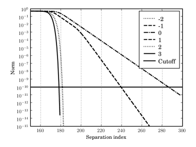
of operator blocks computed via (18). The norms of individual blocks Fiij;m,lsuperscriptsubscript𝐹𝑖superscript𝑖𝑗𝑚𝑙F_{ii^{{}^{\prime}}}^{j;\,m,l} are illustrated in Figure 5 (a), for scale j=1.𝑗1j=1.

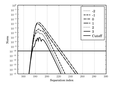
By selecting the number of vanishing moments for a given accuracy, it is sufficient to use 2subscriptnorm2\|\ell\|_{\infty}\leq 2 in practical applications that we have encountered. Also, not all terms in the Gaussian expansion of an operator need to be included since, depending on the scale j𝑗j, their contribution may be negligible for a given accuracy, as shown in Figure 5 (b). Below we detail how we select terms of the Gaussian expansion on a given scale as well as the significant blocks of 𝐓j(𝐓j1)limit-fromsuperscriptsubscript𝐓𝑗superscriptsubscript𝐓𝑗1\mathbf{T}_{j}^{\ell}-\uparrow(\mathbf{T}_{j-1}^{\ell}). This procedure establishes the band structure of the operator. We then project the banded operator (𝐓j1bj)absentsuperscriptsubscript𝐓𝑗1subscript𝑏𝑗\uparrow(\mathbf{T}_{j-1}^{b_{j}}) back to the scale j1𝑗1j-1 and then combine blocks on the natural scale for each projection in order to apply the operator efficiently as was explained in Section 2.3 for the one-dimensional case.

We note that in deciding which terms to keep in (4), we do not compute the difference between the full three dimensional blocks as it would carry a high computational cost; instead we use estimates based on the one dimensional blocks of the separated representation. We note that since the resulting band structure depends only on the operator and the desired accuracy of its approximation, one of the options is to store such band information as it is likely to be reused.

In order to efficiently identify the significant blocks in 𝐓j(𝐓j1)limit-fromsuperscriptsubscript𝐓𝑗superscriptsubscript𝐓𝑗1\mathbf{T}_{j}^{\ell}-\uparrow(\mathbf{T}_{j-1}^{\ell}) as a function of \ell, we develop norm estimates based only on the one-dimensional blocks. The difference between two terms of the separated representation, say F1F2F3G1G2G3subscript𝐹1subscript𝐹2subscript𝐹3subscript𝐺1subscript𝐺2subscript𝐺3F_{1}F_{2}F_{3}-G_{1}G_{2}G_{3}, may be written as

F1F2F3G1G2G3=(F1G1)F2F3+G1(F2G2)F3+G1G2(F3G3).subscript𝐹1subscript𝐹2subscript𝐹3subscript𝐺1subscript𝐺2subscript𝐺3subscript𝐹1subscript𝐺1subscript𝐹2subscript𝐹3subscript𝐺1subscript𝐹2subscript𝐺2subscript𝐹3subscript𝐺1subscript𝐺2subscript𝐹3subscript𝐺3F_{1}F_{2}F_{3}-G_{1}G_{2}G_{3}=(F_{1}-G_{1})F_{2}F_{3}+G_{1}(F_{2}-G_{2})F_{3}+G_{1}G_{2}(F_{3}-G_{3}).

We average six different combinations of the three terms to include all directions in a symmetric manner, which results in the norm estimate

F1F2F3G1G2G3normsubscript𝐹1subscript𝐹2subscript𝐹3subscript𝐺1subscript𝐺2subscript𝐺3\displaystyle\|F_{1}F_{2}F_{3}-G_{1}G_{2}G_{3}\| \displaystyle\leq 16sym[F1G1F2F3+\displaystyle\frac{1}{6}\mbox{sym}\left[\|F_{1}-G_{1}\|\|F_{2}\|\|F_{3}\|+\right.
G1F2G2F3+G1G2F3G3],\displaystyle\left.\|G_{1}\|\|F_{2}-G_{2}\|\|F_{3}\|+\|G_{1}\|\|G_{2}\|\|F_{3}-G_{3}\|\right],

where the symmetrization is over the three directions and generates 181818 terms. For the rotationally symmetric operators with Gaussian expansion as in (15) computing the right hand side in this estimate involves just three types of one dimensional blocks and their norms,

Ndifj;m;lsuperscriptsubscript𝑁dif𝑗𝑚𝑙\displaystyle N_{\mbox{dif}}^{j;m;l} =\displaystyle= Fj;m;l(Fj1;m;l),\displaystyle\left\|F^{j;m;l}-\uparrow(F^{j-1;m;l})\right\|,
NFj;m;lsuperscriptsubscript𝑁𝐹𝑗𝑚𝑙\displaystyle N_{F}^{j;m;l} =\displaystyle= Fj;m;l,normsuperscript𝐹𝑗𝑚𝑙\displaystyle\left\|F^{j;m;l}\right\|, (22)
NFj;m;lsuperscriptsubscript𝑁absent𝐹𝑗𝑚𝑙\displaystyle N_{\uparrow F}^{j;m;l} =\displaystyle= (Fj1;m;l),\displaystyle\left\|\uparrow(F^{j-1;m;l})\right\|,

where index j𝑗j indicates the scale, m𝑚m the term in the Gaussian expansion (15), and l𝑙l the position of the block in a given direction.

These estimates allow us to discard blocks whose norm falls below a given threshold of accuracy, namely, for each multi-index \ell, we estimate

𝐓j(𝐓j1)\displaystyle\left\|\mathbf{T}_{j}^{\ell}-\uparrow(\mathbf{T}_{j-1}^{\ell})\right\| \displaystyle\leq 16m=1Mwmsym[Ndifj;m;l1NFj;m;l2NFj;m;l3+\displaystyle\frac{1}{6}\sum_{m=1}^{M}w_{m}\,\,\mbox{sym}\left[N_{\mbox{dif}}^{j;m;l_{1}}N_{F}^{j;m;l_{2}}N_{F}^{j;m;l_{3}}+\right.
NFj;m;l1Ndifj;m;l2NFj;m;l3+NFj;m;l1NFj;m;l2Ndifj;m;l3].\displaystyle\left.N_{\uparrow F}^{j;m;l_{1}}N_{\mbox{dif}}^{j;m;l_{2}}N_{F}^{j;m;l_{3}}+N_{\uparrow F}^{j;m;l_{1}}N_{\uparrow F}^{j;m;l_{2}}N_{\mbox{dif}}^{j;m;l_{3}}\right].
Refer to caption
(a) Norms of each one-dimensional block computed via (18) for scale j=1𝑗1j=1, as a function of the index m𝑚m in the separated representation.
Refer to caption
(b) Norm estimates (4) for scale j=1𝑗1j=1 as a function of the index m𝑚m in the separated representation. Based on these estimates, only terms above the cutoff are actually applied.
Figure 5: Comparison of norms of matrix blocks generated by the Gaussian approximation for the Poisson kernel in dimension d=3𝑑3d=3. In each picture, the curves correspond to the different offsets l𝑙l for which blocks are generated. Figure (b) illustrates the estimate in (4) (see main text for details).

For each scale j𝑗j and each block 𝐓j(𝐓j1)limit-fromsuperscriptsubscript𝐓𝑗superscriptsubscript𝐓𝑗1\mathbf{T}_{j}^{\ell}-\uparrow(\mathbf{T}_{j-1}^{\ell}) labeled by the multi-index =(l1,l2,l3)subscript𝑙1subscript𝑙2subscript𝑙3\ell=(l_{1},l_{2},l_{3}), we compute all terms of the sum in (4) and identify the range [m1,m2]subscript𝑚1subscript𝑚2[m_{1},m_{2}] which we need to keep for that block, by discarding from the sum terms whose cumulative contribution is below ϵitalic-ϵ\epsilon. If the entire sum falls below ϵitalic-ϵ\epsilon, this range may be empty and the entire 𝐓j(𝐓j1)limit-fromsuperscriptsubscript𝐓𝑗superscriptsubscript𝐓𝑗1\mathbf{T}_{j}^{\ell}-\uparrow(\mathbf{T}_{j-1}^{\ell}) is discarded. The range [m1,m2]subscript𝑚1subscript𝑚2[m_{1},m_{2}] differs significantly depending whether or not the block is affected by the singularity of the kernel as is illustrated in Figure 5. In Figure 5 (a) the rate of decay for the blocks with shift |l|=2,3𝑙23|l|=2,3 is significantly faster than for the blocks with |l|1𝑙1|l|\leq 1 affected by the singularity. We note that all blocks of the first 150 terms in the separated representation (17) have norm 1 (and rank 1 as matrices) and are not shown in Figure 5 (a).

Since the difference in (4) involves blocks upsampled from a coarser scale, all shifts |l|3𝑙3|l|\leq 3 are affected by the singularity. Figure 5 (b) shows the r.h.s. of the estimate in (4) for different shifts along one of the directions, where the blocks along the other two directions are estimated by the maximum norm over all possible shifts.

After discarding blocks with norms less that ϵitalic-ϵ\epsilon using the estimate in (4), we downsample the remaining blocks of (𝐓j1)absentsuperscriptsubscript𝐓𝑗1\uparrow(\mathbf{T}_{j-1}^{\ell}) back to the original scale. This leaves only blocks of 𝐓jsuperscriptsubscript𝐓𝑗\mathbf{T}_{j}^{\ell} on the scale j𝑗j and we remove additional blocks of 𝐓jsuperscriptsubscript𝐓𝑗\mathbf{T}_{j}^{\ell} for the shifts |l|=2,3𝑙23|l|=2,3 where the decay is sufficiently fast to make their contribution less than ϵitalic-ϵ\epsilon.

This leads us to arrange the blocks on each scale into several subsets by the effect the singularity of the kernel has on them and find the appropriate range [m1,m2]subscript𝑚1subscript𝑚2[m_{1},m_{2}] for each subset. There are three such sets in dimension d=2𝑑2d=2 and four sets in dimension d=3𝑑3d=3. For each index l,𝑙l, we will say that the index belongs to the core if l=1,0,1𝑙101l=-1,0,1 and to the boundary otherwise. The core indices correspond to one-dimensional blocks whose defining integrals include the singularity of the kernel. We then divide all possible values of the multi-index =(l1,l2,l3)subscript𝑙1subscript𝑙2subscript𝑙3\ell=(l_{1},l_{2},l_{3}), according to the number of core indices it has. In d=3𝑑3d=3 this gives us four sets:

  • Core: all indices (l1,l2,l3)subscript𝑙1subscript𝑙2subscript𝑙3(l_{1},l_{2},l_{3}) belong to the core.

  • Boundary-1: two of the indices belong to the core and one to the boundary

  • Boundary-2: one of the indices belongs to the core, the other two to the boundary

  • Boundary-3: all indices (l1,l2,l3)subscript𝑙1subscript𝑙2subscript𝑙3(l_{1},l_{2},l_{3}) belong to the boundary.

We then find the range [m1,m2]subscript𝑚1subscript𝑚2[m_{1},m_{2}] for each subset and apply blocks of each subset separately, thus avoiding unnecessary computations with blocks whose contribution is negligible. This range analysis only needs to be done once per operator and the desired accuracy, and the results may be saved for repeated use.

5 Multidimensional adaptive application of ns-form

In this section we present an algorithm for applying the modified non-standard form which is an extension of (2) (based on (8) and (2.4)) to higher dimensions. We are now seeking to compute

g(𝐱)=[Tf](𝐱)=K(𝐲𝐱)f(𝐲)𝑑𝐲,𝑔𝐱delimited-[]𝑇𝑓𝐱𝐾𝐲𝐱𝑓𝐲differential-d𝐲g(\mathbf{x})=[Tf](\mathbf{x})=\int K(\mathbf{y}-\mathbf{x})f(\mathbf{y})d\mathbf{y},

where 𝐱,𝐲d𝐱𝐲superscript𝑑\mathbf{x},\mathbf{y}\in\mathbb{R}^{d} for d=2,3𝑑23d=2,3. The separated approximation (4) reduces the complexity of applying the operator by allowing partial factorization of the nested loops in each scale indicated by the order of summation and illustrated for d=3𝑑3d=3,

gj;l1l2l3superscript𝑔𝑗subscript𝑙1subscript𝑙2subscript𝑙3\displaystyle g^{j;l_{1}l_{2}l_{3}} =\displaystyle= mwm{l1Fj;m;l1l1l2Fj;m,l2l2l3Fj;m,l3l3\displaystyle\sum_{m}w_{m}\left\{\sum_{l^{\prime}_{1}}F^{j;m;l_{1}-l^{\prime}_{1}}\sum_{l^{\prime}_{2}}F^{j;m,l_{2}-l^{\prime}_{2}}\sum_{l^{\prime}_{3}}F^{j;m,l_{3}-l^{\prime}_{3}}\right.-
[l1Fj1;m;l1l1l2Fj1;m,l2l2l3Fj1;m,l3l3]}fj;l1l2l3.\displaystyle\left.\uparrow\left[\sum_{l^{\prime}_{1}}F^{j-1;m;l_{1}-l^{\prime}_{1}}\sum_{l^{\prime}_{2}}F^{j-1;m,l_{2}-l^{\prime}_{2}}\sum_{l^{\prime}_{3}}F^{j-1;m,l_{3}-l^{\prime}_{3}}\right]\right\}f^{j;l^{\prime}_{1}l^{\prime}_{2}l^{\prime}_{3}}.

As described in the previous section, this evaluation is done by regions of indices. These regions of indices are organized so that (for a given accuracy) the number of retained terms of the separated representation is roughly the same for all blocks within each region. Thus, we perform the summation over the terms of the separated representation last, applying only the terms that actually contribute to the result above the requested accuracy threshold, according to estimate (4). Therefore, we avoid introducing checks per individual block and the resulting loss of performance.

Just as in the one-dimensional case, we use (4) in a ‘natural scale’ manner. That is, blocks belonging to scale j𝑗j are only applied on that scale. As in one-dimensional case, the interaction between scales is achieved by the projection (2.4) that redistributes blocks accumulated in this manner properly between the scales to obtain the adaptive tree for the resulting function. The overall approach is the same as described in (2). We note that, as expected, the separated representation requires more detailed bookkeeping when constructing the data structures for the operator.

Remark 1

Our multiresolution decomposition corresponds to the geometrically varying refinement in finite element methods. In this case the adjoining boxes do not necessarily share common vertices, forming what corresponds to the so-called non-conforming grid. In finite element methods such situation requires additional construction provided by the mortar element methods. Mortar element methods were introduced by Patera and his associates, see e.g. [19, 20, 21, 22]. These methods permit coupling discretizations of different types in non-overlapping domains. Such methods are fairly complicated and involve, for example, the introduction of interface conditions through an L2superscript𝐿2L^{2} minimization. In our approach we do not face these issues at all and do not have to introduce any additional interface conditions. The proper construction for adjoining boxes is taken care by the redundant tree data structure and Step 2 of Algorithm 3 for applying the kernel, which generates the necessary missing boxes on appropriate scales.

Remark 2

Although Algorithm 3 applies convolution operators, only minor changes are needed to use it for non-convolutions. Of course in such case, the separated representation for the modified ns-form should be constructed by a different approach.

Algorithm 3 Adaptive non-standard form operator application in multiple dimensions (illustrated for d=2𝑑2d=2), g=𝐓f𝑔𝐓𝑓g=\mathbf{T}f
  Initialization: Construct the redundant tree for f𝑓f and copy it as skeleton tree for g𝑔g (see Section 2.2.1).
  for all scales j=0,,n1𝑗0𝑛1j=0,\ldots,n-1 do
     for all function blocks gl1l2jsuperscriptsubscript𝑔subscript𝑙1subscript𝑙2𝑗g_{l_{1}l_{2}}^{j} in the tree for g𝑔g at scale j𝑗j do
        # Step 1. Determine the list of all Core, Boundary-1 and Boundary-2 contributing operator blocks of the modified ns-form Fj;m;l1l1,Fj;m;l2l2superscript𝐹𝑗𝑚subscript𝑙1superscriptsubscript𝑙1superscript𝐹𝑗𝑚subscript𝑙2superscriptsubscript𝑙2F^{j;m;l_{1}-l_{1}^{\prime}},F^{j;m;l_{2}-l_{2}^{\prime}} (see Section 4):
        if gl1l2jsuperscriptsubscript𝑔subscript𝑙1subscript𝑙2𝑗g_{l_{1}l_{2}}^{j} belongs to a leaf then
           Read operator blocks Fj;m;l1l1,Fj;m;l2l2superscript𝐹𝑗𝑚subscript𝑙1superscriptsubscript𝑙1superscript𝐹𝑗𝑚subscript𝑙2superscriptsubscript𝑙2F^{j;m;l_{1}-l_{1}^{\prime}},F^{j;m;l_{2}-l_{2}^{\prime}} for Core, Boundary-1 and Boundary-2, and their weights wmsubscript𝑤𝑚w_{m} and corresponding ranges from the separated representation.
        else
           Read operator blocks Fj;m;l1l1,Fj;m;l2l2superscript𝐹𝑗𝑚subscript𝑙1superscriptsubscript𝑙1superscript𝐹𝑗𝑚subscript𝑙2superscriptsubscript𝑙2F^{j;m;l_{1}-l_{1}^{\prime}},F^{j;m;l_{2}-l_{2}^{\prime}} for Boundary-1 and Boundary-2, and their weights wmsubscript𝑤𝑚w_{m} and corresponding ranges from the separated representation.
        end if
        # Step 2. Find the required blocks fl1l2jsuperscriptsubscript𝑓superscriptsubscript𝑙1superscriptsubscript𝑙2𝑗{f_{l_{1}^{\prime}l_{2}^{\prime}}^{j}} of the input function f𝑓f:
        if function block fl1l2jsuperscriptsubscript𝑓superscriptsubscript𝑙1superscriptsubscript𝑙2𝑗{f_{l_{1}^{\prime}l_{2}^{\prime}}^{j}} exists in the redundant tree for f𝑓f then
           Retrieve it.
        else
           Create it by interpolating from a coarser scale and cache for reuse.
        end if
        # Step 3. Output function block computation:
        For each set S𝑆S of indices determined in Step 1 (Core, Boundary-1, Boundary-2) and the corresponding ranges of terms in the separated representation, compute the sum
g^l1l2j;S=mwml1Fj;m;l1l1l2Fj;m;l2l2fl1l2j,superscriptsubscript^𝑔subscript𝑙1subscript𝑙2𝑗𝑆subscript𝑚subscript𝑤𝑚subscriptsuperscriptsubscript𝑙1superscript𝐹𝑗𝑚subscript𝑙1superscriptsubscript𝑙1subscriptsuperscriptsubscript𝑙2superscript𝐹𝑗𝑚subscript𝑙2superscriptsubscript𝑙2superscriptsubscript𝑓superscriptsubscript𝑙1superscriptsubscript𝑙2𝑗\hat{g}_{l_{1}l_{2}}^{j;S}=\sum_{m}w_{m}\sum_{l_{1}^{\prime}}F^{j;m;l_{1}-l_{1}^{\prime}}\sum_{l_{2}^{\prime}}F^{j;m;l_{2}-l_{2}^{\prime}}f_{l_{1}^{\prime}l_{2}^{\prime}}^{j},
        Add all computed sums to obtain g^l1l2jsuperscriptsubscript^𝑔subscript𝑙1subscript𝑙2𝑗\hat{g}_{l_{1}l_{2}}^{j}.
     end for
  end for
  # Step 4. Adaptive projection:
  Project resulting output function blocks g^l1l2jsuperscriptsubscript^𝑔subscript𝑙1subscript𝑙2𝑗\hat{g}_{l_{1}l_{2}}^{j} on all scales into a proper adaptive tree by using Eq. (5).
  Discard from the resulting tree unnecessary function blocks at the requested accuracy.
  Return: the function g𝑔g represented by its adaptive tree.

5.1 Operation count estimates

Adaptive decomposition of functions

The cost of adaptively decomposing a function in d𝑑d dimensions is essentially that of an adaptive wavelet transform. Specifically, it takes 𝒪(Nblockspd+1)𝒪subscript𝑁blockssuperscript𝑝𝑑1\mathcal{O}(N_{\textrm{blocks}}\cdot p^{d+1}) operations to compute such representation, where Nblockssubscript𝑁blocksN_{\textrm{blocks}} is the final number of significant blocks in the representation and p𝑝p is the order of multiwavelet basis chosen. In comparison with the usual wavelet transform, it appears to be significantly more expensive. However, these 𝒪(pd+1)𝒪superscript𝑝𝑑1\mathcal{O}(p^{d+1}) operations process 𝒪(pd)𝒪superscript𝑝𝑑\mathcal{O}(p^{d}) points, thus in counting significant coefficients as it is done in the usual adaptive wavelet transform, we end up with 𝒪(p)𝒪𝑝\mathcal{O}(p) operations per point.

Operator application

The cost of applying an operator in the modified ns-form is 𝒪(NblocksMpd+1)𝒪subscript𝑁blocks𝑀superscript𝑝𝑑1\mathcal{O}(N_{\textrm{blocks}}Mp^{d+1}), where Nblockssubscript𝑁blocksN_{\textrm{blocks}} is the number of blocks in the adaptive representation of the input function, M𝑀M is the separation rank of the kernel in (15) and p𝑝p is the order of the multiwavelet basis. For a given desired accuracy ϵitalic-ϵ\epsilon, we typically select plogϵ1proportional-to𝑝superscriptitalic-ϵ1p\propto\log\epsilon^{-1}; M𝑀M has been shown to be proportional to (logϵ1)νsuperscriptsuperscriptitalic-ϵ1𝜈(\log\epsilon^{-1})^{\nu}, where ν𝜈\nu depends on the operator [24]. In our numerical experiments, M𝑀M is essentially proportional to logϵ1superscriptitalic-ϵ1\log\epsilon^{-1}, since we never use the full separated representation, as discussed in Section 4 and illustrated in Figure 5.

This operation count can be potentially reduced to 𝒪(NblocksMpd)𝒪subscript𝑁blocks𝑀superscript𝑝𝑑\mathcal{O}(N_{\textrm{blocks}}Mp^{d}) by using the structure of the matrices in 18, and we plan to address this in the future.

Final projection

After the operator has been applied to a function in a scale-independent fashion, a final projection step is required as discussed in Section 2.3. This step requires 𝒪(Nblockspd)𝒪subscript𝑁blockssuperscript𝑝𝑑\mathcal{O}(N_{\textrm{blocks}}\cdot p^{d}) operations, the same as in the original function decomposition. In practice, this time is negligible compared to the actual operator application.

6 Numerical examples

6.1 The Poisson equation

We illustrate the performance of the algorithm by solving the Poisson equation in d=3𝑑3d=3

2ϕ(𝐫)=ρ(𝐫)superscript2italic-ϕ𝐫𝜌𝐫\nabla^{2}\phi(\mathbf{r})=-\rho(\mathbf{r}) (24)

with free space boundary conditions, ϕ(𝐫)0italic-ϕ𝐫0\phi(\mathbf{r})\to 0 and ϕ/r0italic-ϕ𝑟0\partial\phi/\partial r\to 0 as r𝑟r\to\infty. We write the solution as

ϕ(𝐫)=14π31|𝐫𝐫|ρ(𝐫)𝑑𝐫italic-ϕ𝐫14𝜋subscriptsuperscript31𝐫superscript𝐫𝜌superscript𝐫differential-dsuperscript𝐫\phi(\mathbf{r})=\frac{1}{4\pi}\int_{\mathbb{R}^{3}}\frac{1}{\left|\mathbf{r}-\mathbf{r}^{\prime}\right|}\rho(\mathbf{r}^{\prime})d\mathbf{r}^{\prime}

and adaptively evaluate this integral. We note that our method can equally be used for d=2,𝑑2d=2, since the corresponding Green’s function can also be represented as a sum of Gaussians, and the operator application algorithm has been implemented in for both d=2𝑑2d=2 and d=3𝑑3d=3.

For our test we select

ϕ(𝐫)=i=13eα|𝐫𝐫|2,italic-ϕ𝐫superscriptsubscript𝑖13superscript𝑒𝛼superscript𝐫superscript𝐫2\phi(\mathbf{r})=\sum_{i=1}^{3}e^{-\alpha\left|\mathbf{r}-\mathbf{r}^{\prime}\right|^{2}},

so that we solve the Poisson equation with

ρ(𝐫)=2ϕ(𝐫)=i=13(4α2|𝐫𝐫i|26α)eα|𝐫𝐫i|2.𝜌𝐫superscript2italic-ϕ𝐫superscriptsubscript𝑖134superscript𝛼2superscript𝐫subscript𝐫𝑖26𝛼superscript𝑒𝛼superscript𝐫subscript𝐫𝑖2\rho(\mathbf{r})=-\nabla^{2}\phi(\mathbf{r})=-\sum_{i=1}^{3}(4\alpha^{2}\left|\mathbf{r}-\mathbf{r}_{i}\right|^{2}-6\alpha)e^{-\alpha\left|\mathbf{r}-\mathbf{r}_{i}\right|^{2}}.

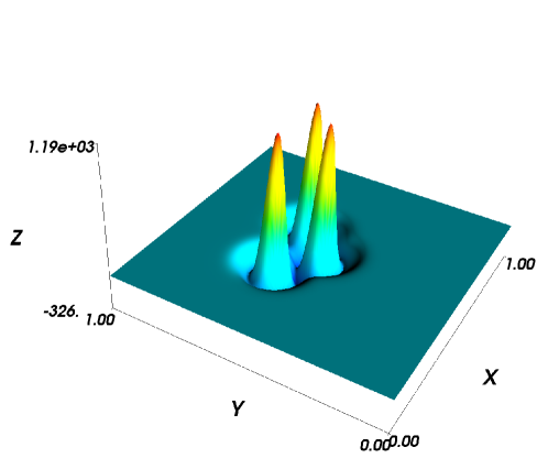
Our parameters are chosen as follows: α=300𝛼300\alpha=300, r1=(0.5,0.5,0.5),subscript𝑟10.50.50.5r_{1}=(0.5,0.5,0.5), r2=(0.6,0.6,0.5)subscript𝑟20.60.60.5r_{2}=(0.6,0.6,0.5) and r3=(0.35,0.6,0.5).subscript𝑟30.350.60.5r_{3}=(0.35,0.6,0.5). These ensure that ρ(r)𝜌𝑟\rho(r) is well below our requested thresholds on the boundary of the computational domain. All numerical experiments were performed on a Pentium-4 running at 2.8 GHz, with 2 GB of RAM. The results are summarized in Table 2.

In order to gauge the speed of algorithm in reasonably computer-independent terms, we use a similar approach to that of [17] and also provide timings of the Fast Fourier Transform (FFT). Specifically, we display timings for two FFTs as an estimate of the time needed to solve the Poisson equation with a smooth right hand side and periodic boundary conditions in a cube. As in [17], we compute the rate that estimates the number of processed points per second. We observe that for our adaptive algorithm such rate varies between 3.41043.4superscript1043.4\cdot 10^{4} and 1.11051.1superscript1051.1\cdot 10^{5} (see Table 2), whereas for the FFTs it is around 106superscript10610^{6} (see Table 3). We note that our algorithm is not fully optimized, namely, we do not use the structure of the matrices in (18) and the symmetries afforded by the radial kernels. We expect a substantial impact on the speed by introducing these improvements and will report them separately.

We note that the multigrid method (see e.g. [28, 29]) is frequently used as a tool for solving the Poisson equation (and similar problems) in differential form. The FFT-based gauge suggested in [17] is useful for comparisons with these algorithms as well.

Requested ϵ=103italic-ϵsuperscript103\epsilon=10^{-3}

p𝑝p E2subscript𝐸2E_{2} Esubscript𝐸E_{\infty} Time (s) Rate (pts/s)
6 5.01035.0superscript1035.0\cdot 10^{-3} 7.91017.9superscript1017.9\cdot 10^{-1} 1.21.21.2 7.21047.2superscript1047.2\cdot 10^{4}
8 1.71031.7superscript1031.7\cdot 10^{-3} 1.21011.2superscript1011.2\cdot 10^{-1} 0.510.510.51 7.31047.3superscript1047.3\cdot 10^{4}
10 4.41044.4superscript1044.4\cdot 10^{-4} 3.71023.7superscript1023.7\cdot 10^{-2} 0.680.680.68 1.11051.1superscript1051.1\cdot 10^{5}

Requested ϵ=106italic-ϵsuperscript106\epsilon=10^{-6}

p𝑝p E2subscript𝐸2E_{2} Esubscript𝐸E_{\infty} Time (s) Rate (pts/s)
10 4.71064.7superscript1064.7\cdot 10^{-6} 3.61043.6superscript1043.6\cdot 10^{-4} 10.3 5.71045.7superscript1045.7\cdot 10^{4}
12 8.51068.5superscript1068.5\cdot 10^{-6} 4.31054.3superscript1054.3\cdot 10^{-5} 13.5 7.51047.5superscript1047.5\cdot 10^{4}
14 6.91086.9superscript1086.9\cdot 10^{-8} 5.21065.2superscript1065.2\cdot 10^{-6} 20.0 8.01048.0superscript1048.0\cdot 10^{4}

Requested ϵ=109italic-ϵsuperscript109\epsilon=10^{-9}

p𝑝p E2subscript𝐸2E_{2} Esubscript𝐸E_{\infty} Time (s) Rate (pts/s)
16 2.510102.5superscript10102.5\cdot 10^{-10} 2.21082.2superscript1082.2\cdot 10^{-8} 68.1 3.51043.5superscript1043.5\cdot 10^{4}
18 7.710117.7superscript10117.7\cdot 10^{-11} 3.51093.5superscript1093.5\cdot 10^{-9} 100.3 3.41043.4superscript1043.4\cdot 10^{4}
20 1.210101.2superscript10101.2\cdot 10^{-10} 1.81081.8superscript1081.8\cdot 10^{-8} 133.4 3.51043.5superscript1043.5\cdot 10^{4}
Table 2: Accuracy and timings for the adaptive solution of the Poisson equation in (24).
size Time (s) Rate (pts/s)
323superscript32332^{3} 0.02 1.71061.7superscript1061.7\cdot 10^{6}
643superscript64364^{3} 0.22 1.21061.2superscript1061.2\cdot 10^{6}
1283superscript1283128^{3} 2.21 9.51059.5superscript1059.5\cdot 10^{5}
2563superscript2563256^{3} 20.7 8.11058.1superscript1058.1\cdot 10^{5}

Table 3: Timings of two 3D FFTs to estimate the speed of a non-adaptive, periodic Poisson solver on a cube for smooth functions.
Refer to caption
Refer to caption
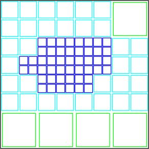
Figure 6: A two-dimensional slice of the three-dimensional subdivision of space by the scaling functions and an illustration of the source term for the Poisson equation (24).

6.2 The ground state of the hydrogen atom

A simple example of computing the ground state of the hydrogen atom illustrates the numerical performance of the algorithms developed in this paper, and their utility for constructing more complex codes. The eigenfunctions ψ𝜓\psi for the hydrogen atom satisfy the time-independent Schrödinger equation (written in atomic units and spherical coordinates),

12Δψ1rψ=Eψ,12Δ𝜓1𝑟𝜓𝐸𝜓-\frac{1}{2}\Delta\psi-\frac{1}{r}\psi=E\psi, (25)

where E𝐸E is the energy eigenvalue. For the ground state, E=1/2𝐸12E=-1/2 and the (unnormalized) wave function is ψ=er𝜓superscript𝑒𝑟\psi=e^{-r}. Following [30], we write

ϕ=2GμVϕ,italic-ϕ2subscript𝐺𝜇𝑉italic-ϕ\phi=-2G_{\mu}V\phi, (26)

where Gμ=(Δ+μ2)1subscript𝐺𝜇superscriptΔsuperscript𝜇21G_{\mu}=(-\Delta+\mu^{2}\mathcal{I})^{-1} is the Green’s function for some μ𝜇\mu and V=1/r𝑉1𝑟V=-1/r is the nuclear potential. For μ=2E𝜇2𝐸\mu=\sqrt{-2E} the solution ϕitalic-ϕ\phi of (26) has ϕ2=1subscriptnormitalic-ϕ21\|\phi\|_{2}=1 and coincides with that of (25). We solve (26) by a simple iteration starting from some value μ0subscript𝜇0\mu_{0} and changing μ𝜇\mu to obtain the solution with ϕ2=1subscriptnormitalic-ϕ21\|\phi\|_{2}=1. The algorithm proceeds as follows:

  1. 1.

    Initialize with some value μ0subscript𝜇0\mu_{0} and function ϕitalic-ϕ\phi. The number of iterations of the algorithm is only weakly sensitive to these choices.

  2. 2.

    Compute the product of the potential V𝑉V and the function ϕitalic-ϕ\phi.

  3. 3.

    Apply the Green’s function Gμsubscript𝐺𝜇G_{\mu} to the product Vϕ𝑉italic-ϕV\phi via the algorithm of this paper to compute

    ϕnew=2GμVϕ.subscriptitalic-ϕ𝑛𝑒𝑤2subscript𝐺𝜇𝑉italic-ϕ\phi_{new}=-2G_{\mu}V\phi.
  4. 4.

    Compute the energy for ϕnewsubscriptitalic-ϕ𝑛𝑒𝑤\phi_{new},

    Enew=12ϕnew,ϕnew+Vϕnew,ϕnewϕnew,ϕnew.subscript𝐸𝑛𝑒𝑤12subscriptitalic-ϕ𝑛𝑒𝑤subscriptitalic-ϕ𝑛𝑒𝑤𝑉subscriptitalic-ϕ𝑛𝑒𝑤subscriptitalic-ϕ𝑛𝑒𝑤subscriptitalic-ϕ𝑛𝑒𝑤subscriptitalic-ϕ𝑛𝑒𝑤E_{new}=\frac{\frac{1}{2}\langle\nabla\phi_{new},\nabla\phi_{new}\rangle+\langle V\phi_{new},\phi_{new}\rangle}{\langle\phi_{new},\phi_{new}\rangle}.
  5. 5.

    Set μ=2Enew𝜇2subscript𝐸𝑛𝑒𝑤\mu=\sqrt{-2E_{new}}, ϕ=ϕnew/ϕnewitalic-ϕsubscriptitalic-ϕ𝑛𝑒𝑤normsubscriptitalic-ϕ𝑛𝑒𝑤\phi=\phi_{new}/\|\phi_{new}\| and return to Step 2.

The iteration is terminated as the change in μ𝜇\mu and ϕ1normitalic-ϕ1\|\phi\|-1 falls below the desired accuracy. The progress of the iteration is illustrated in Figure 7. The computations in Steps 2 and 4 use the three dimensional extension of the approach described in [13], to compute point-wise multiplications of adaptively represented functions and weak differential operators of the same.

This example illustrates an application of our algorithm to problems in quantum chemistry. Multiresolution quantum chemistry developed in [8, 9, 10, 11] also uses separated representations. The main technical difference with [8, 9, 10, 11] is that we use the modified non-standard form and apply operator blocks on their “natural” scale, thus producing a fully adaptive algorithm. We are currently using this algorithm as part of a new method for solving the multiparticle Schrödinger equation and will report the results elsewhere.
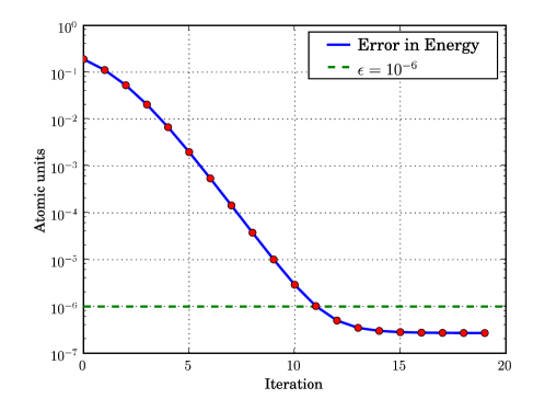
Refer to caption
Figure 7: Convergence of the iteration to obtain the ground state of the hydrogen atom computed via formulation in (26) for the non-relativistic Schrödinger equation. The requested accuracy in applying the Green’s function is set to 106superscript10610^{-6}.

7 Discussion and conclusions

We have shown that a combination of separated and multiresolution representations of operators yields a new multidimensional algorithm for applying a class of integral operators with radial kernels. We note that the same algorithm is used for all such operators as they are approximated by a weighted sum of Gaussians. This fact makes our approach applicable across multiple fields, where a single implementation of the core algorithm can be reused for different specific problems. The algorithm is fully adaptive and avoids issues usually addressed by mortar methods.

The method of approximation underlying our approach is distinct from that of the FMM, has similar efficiency and has the advantage of being more readily extendable to higher dimensions. We also note that semi-analytic approximations via weighted sums of Gaussians provide additional advantages in some applications. Although we described the application of kernels in free space, there is a simple extension to problems with radial kernels subject to periodic, Dirichlet or Neumann boundary conditions on a cube that we will describe separately.

The algorithm may be extended to classes of non-convolution operators, e.g., the Calderon-Zygmund operators. For such extensions the separated representation may not be available in analytic form, as it is for the operators of this paper, and may require a numerical construction. The separated representation of the kernel permits further generalization of our approach to dimensions d3much-greater-than𝑑3d\gg 3 for applying operators to functions in separated representation.

A notable remaining challenge is an efficient, high order extension of this technique to the application of operators on domains with complicated geometries and surfaces.

8 Appendix

8.1 Scaling functions

We use either the Legendre polynomials P0,,Pp1subscript𝑃0subscript𝑃𝑝1P_{0},\ldots,P_{p-1} or the interpolating polynomials on the Gauss-Legendre nodes in [1,1]11[-1,1] to construct an orthonormal basis for each subspace 𝐕jsubscript𝐕𝑗\mathbf{V}_{j} [12, 13].

Let us briefly describe some properties of the Legendre scaling functions ϕksubscriptitalic-ϕ𝑘\phi_{k}, k=0,,p1𝑘0𝑝1k=0,\ldots,p-1, defined as

ϕk(x)={2k+1Pk(2x1),x[0,1]0,x[0,1],subscriptitalic-ϕ𝑘𝑥cases2𝑘1subscript𝑃𝑘2𝑥1𝑥010𝑥01\phi_{k}(x)=\left\{\begin{array}[]{ll}\sqrt{2k+1}P_{k}(2x-1),&x\in[0,1]\\ 0,&x\notin[0,1]\end{array}\right., (27)

and forming a basis for 𝐕0.subscript𝐕0\mathbf{V}_{0}. The subspace 𝐕jsubscript𝐕𝑗\mathbf{V}_{j} is spanned by 2jpsuperscript2𝑗𝑝2^{j}p functions obtained from ϕ0,,ϕp1subscriptitalic-ϕ0subscriptitalic-ϕ𝑝1\phi_{0},\ldots,\phi_{p-1} by dilation and translation,

ϕklj(x)=2j/2ϕk(2jxl),k=0,,p1,l=0,,2j1.formulae-sequencesuperscriptsubscriptitalic-ϕ𝑘𝑙𝑗𝑥superscript2𝑗2subscriptitalic-ϕ𝑘superscript2𝑗𝑥𝑙formulae-sequence𝑘0𝑝1𝑙0superscript2𝑗1\phi_{kl}^{j}(x)=2^{j/2}\phi_{k}(2^{j}x-l),\quad k=0,\ldots,p-1,\quad l=0,\ldots,2^{j}-1. (28)

These functions have support on [2jl,2j(l+1)]superscript2𝑗𝑙superscript2𝑗𝑙1[2^{-j}l,2^{-j}(l+1)] and satisfy the orthonormality condition

ϕklj(x)ϕklj(x)𝑑x=δkkδll.superscriptsubscriptsuperscriptsubscriptitalic-ϕ𝑘𝑙𝑗𝑥superscriptsubscriptitalic-ϕsuperscript𝑘superscript𝑙𝑗𝑥differential-d𝑥subscript𝛿𝑘superscript𝑘subscript𝛿𝑙superscript𝑙\int_{-\infty}^{\infty}\phi_{kl}^{j}(x)\phi_{k^{\prime}l^{\prime}}^{j}(x)dx=\delta_{kk^{\prime}}\delta_{ll^{\prime}}\,. (29)

A function f𝑓f, defined on [0,1]01[0,1], is represented in the subspace 𝐕jsubscript𝐕𝑗\mathbf{V}_{j} by its normalized Legendre expansion

f(x)=l=02j1k=0p1skljϕklj(x),𝑓𝑥superscriptsubscript𝑙0superscript2𝑗1superscriptsubscript𝑘0𝑝1superscriptsubscript𝑠𝑘𝑙𝑗superscriptsubscriptitalic-ϕ𝑘𝑙𝑗𝑥f(x)=\sum_{l=0}^{2^{j}-1}\sum_{k=0}^{p-1}s_{kl}^{j}\phi_{kl}^{j}(x), (30)

where the coefficients skljsuperscriptsubscript𝑠𝑘𝑙𝑗s_{kl}^{j} are computed via

sklj=2jl2j(l+1)f(x)ϕklj(x)𝑑x.superscriptsubscript𝑠𝑘𝑙𝑗superscriptsubscriptsuperscript2𝑗𝑙superscript2𝑗𝑙1𝑓𝑥superscriptsubscriptitalic-ϕ𝑘𝑙𝑗𝑥differential-d𝑥s_{kl}^{j}=\int_{2^{-j}l}^{2^{-j}(l+1)}f(x)\phi_{kl}^{j}(x)\,dx. (31)

As long as f(x)𝑓𝑥f(x) is smooth enough and is well approximated on [2jl,2j(l+1)]superscript2𝑗𝑙superscript2𝑗𝑙1[2^{-j}l,2^{-j}(l+1)] by a polynomial of order up to 2p12𝑝12p-1, we may use Gauss-Legendre quadratures to calculate the skljsuperscriptsubscript𝑠𝑘𝑙𝑗s_{kl}^{j} via

sklj=2j/2i=0p1f(2j(xi+l))ϕk(xi)wi,superscriptsubscript𝑠𝑘𝑙𝑗superscript2𝑗2superscriptsubscript𝑖0𝑝1𝑓superscript2𝑗subscript𝑥𝑖𝑙subscriptitalic-ϕ𝑘subscript𝑥𝑖subscript𝑤𝑖s_{kl}^{j}=2^{-j/2}\sum_{i=0}^{p-1}f(2^{-j}(x_{i}+l))\phi_{k}(x_{i})w_{i}, (32)

where x0,,xp1subscript𝑥0subscript𝑥𝑝1x_{0},\ldots,x_{p-1} are the roots of Pp(2x1)subscript𝑃𝑝2𝑥1P_{p}(2x-1) and w0,,wp1subscript𝑤0subscript𝑤𝑝1w_{0,}\ldots,w_{p-1} are the corresponding quadrature weights.

In more than one dimension, the above formulas are extended by using a tensor product basis in each subspace. For example, in two dimensions equation (30) becomes

f(x,x)=l=02j1k=0p1l=02j1k=0p1skklljϕklj(x)ϕklj(x).𝑓𝑥superscript𝑥superscriptsubscript𝑙0superscript2𝑗1superscriptsubscript𝑘0𝑝1superscriptsubscriptsuperscript𝑙0superscript2𝑗1superscriptsubscriptsuperscript𝑘0𝑝1superscriptsubscript𝑠𝑘superscript𝑘𝑙superscript𝑙𝑗superscriptsubscriptitalic-ϕ𝑘𝑙𝑗𝑥superscriptsubscriptitalic-ϕsuperscript𝑘superscript𝑙𝑗superscript𝑥f(x,x^{\prime})=\sum_{l=0}^{2^{j}-1}\sum_{k=0}^{p-1}\sum_{l^{\prime}=0}^{2^{j}-1}\sum_{k^{\prime}=0}^{p-1}s_{kk^{\prime}ll^{\prime}}^{j}\phi_{kl}^{j}(x)\phi_{k^{\prime}l^{\prime}}^{j}(x^{\prime}). (33)

8.2 Multiwavelets

We use piecewise polynomial functions ψ0,,ψp1subscript𝜓0subscript𝜓𝑝1\psi_{0,}\ldots,\psi_{p-1} as an orthonormal basis for 𝐖0subscript𝐖0\mathbf{W}_{0} [12, 13],

01ψi(x)ψj(x)𝑑x=δij.superscriptsubscript01subscript𝜓𝑖𝑥subscript𝜓𝑗𝑥differential-d𝑥subscript𝛿𝑖𝑗\int_{0}^{1}\psi_{i}(x)\psi_{j}(x)dx=\delta_{ij}. (34)

Since 𝐖0𝐕0perpendicular-tosubscript𝐖0subscript𝐕0\mathbf{W}_{0}\perp\mathbf{V}_{0}, the first p𝑝p moments of all ψ0,,ψp1subscript𝜓0subscript𝜓𝑝1\psi_{0,}\ldots,\psi_{p-1} vanish:

01ψi(x)xi𝑑x=0,i,j=0,1,,p1.formulae-sequencesuperscriptsubscript01subscript𝜓𝑖𝑥superscript𝑥𝑖differential-d𝑥0𝑖𝑗01𝑝1\int_{0}^{1}\psi_{i}(x)x^{i}dx=0,\quad i,j=0,1,\ldots,p-1. (35)

The space 𝐖jsubscript𝐖𝑗\mathbf{W}_{j} is spanned by 2jpsuperscript2𝑗𝑝2^{j}p functions obtained from ψ0,,ψp1subscript𝜓0subscript𝜓𝑝1\psi_{0,}\ldots,\psi_{p-1} by dilation and translation,

ψklj(x)=2j/2ψk(2jxl),k=0,,p1,l=0,,2j1,formulae-sequencesuperscriptsubscript𝜓𝑘𝑙𝑗𝑥superscript2𝑗2subscript𝜓𝑘superscript2𝑗𝑥𝑙formulae-sequence𝑘0𝑝1𝑙0superscript2𝑗1\psi_{kl}^{j}(x)=2^{j/2}\psi_{k}(2^{j}x-l),\quad k=0,\ldots,p-1,\quad l=0,\ldots,2^{j}-1, (36)

and supported in the interval Ijl=[2jl,2j(l+1)].subscript𝐼𝑗𝑙superscript2𝑗𝑙superscript2𝑗𝑙1I_{jl}=[2^{-j}l,2^{-j}(l+1)]. A function f(x)𝑓𝑥f(x) defined on [0,1]01[0,1] is represented in the multiwavelet basis on n𝑛n scales by

f(x)=k=0p1sk,00ϕk(x)+j=0n1l=02j1k=0p1dkljψklj(x)𝑓𝑥superscriptsubscript𝑘0𝑝1superscriptsubscript𝑠𝑘00subscriptitalic-ϕ𝑘𝑥superscriptsubscript𝑗0𝑛1superscriptsubscript𝑙0superscript2𝑗1superscriptsubscript𝑘0𝑝1superscriptsubscript𝑑𝑘𝑙𝑗superscriptsubscript𝜓𝑘𝑙𝑗𝑥f(x)=\sum_{k=0}^{p-1}s_{k,0}^{0}\phi_{k}(x)+\sum_{j=0}^{n-1}\sum_{l=0}^{2^{j}-1}\sum_{k=0}^{p-1}d_{kl}^{j}\psi_{kl}^{j}(x) (37)

with the coefficients dkljsuperscriptsubscript𝑑𝑘𝑙𝑗d_{kl}^{j} computed via

dklj=2jl2j(l+1)f(x)ψklj(x)𝑑x.superscriptsubscript𝑑𝑘𝑙𝑗superscriptsubscriptsuperscript2𝑗𝑙superscript2𝑗𝑙1𝑓𝑥superscriptsubscript𝜓𝑘𝑙𝑗𝑥differential-d𝑥d_{kl}^{j}=\int_{2^{-j}l}^{2^{-j}(l+1)}f(x)\psi_{kl}^{j}(x)\,dx. (38)

8.3 Two-scale relations

The relation between subspaces, 𝐕0𝐖0=𝐕1direct-sumsubscript𝐕0subscript𝐖0subscript𝐕1\mathbf{V}_{0}\oplus\mathbf{W}_{0}=\mathbf{V}_{1}, is expressed via the two-scale difference equations,

ϕk(x)subscriptitalic-ϕ𝑘𝑥\displaystyle\phi_{k}(x) =\displaystyle= 2k=0p1(hkk(0)ϕk(2x)+hkk(1)ϕk(2x1)),k=0,,p1,formulae-sequence2superscriptsubscriptsuperscript𝑘0𝑝1superscriptsubscript𝑘superscript𝑘0subscriptitalic-ϕsuperscript𝑘2𝑥superscriptsubscript𝑘superscript𝑘1subscriptitalic-ϕsuperscript𝑘2𝑥1𝑘0𝑝1\displaystyle\sqrt{2}\sum_{k^{\prime}=0}^{p-1}\left(h_{kk^{\prime}}^{(0)}\phi_{k^{\prime}}(2x)+h_{kk^{\prime}}^{(1)}\phi_{k^{\prime}}(2x-1)\right),\quad k=0,\ldots,p-1, (39)
ψk(x)subscript𝜓𝑘𝑥\displaystyle\psi_{k}(x) =\displaystyle= 2k=0p1(gkk(0)ϕk(2x)+gkk(1)ϕk(2x1)),k=0,,p1,formulae-sequence2superscriptsubscriptsuperscript𝑘0𝑝1superscriptsubscript𝑔𝑘superscript𝑘0subscriptitalic-ϕsuperscript𝑘2𝑥superscriptsubscript𝑔𝑘superscript𝑘1subscriptitalic-ϕsuperscript𝑘2𝑥1𝑘0𝑝1\displaystyle\sqrt{2}\sum_{k^{\prime}=0}^{p-1}\left(g_{kk^{\prime}}^{(0)}\phi_{k^{\prime}}(2x)+g_{kk^{\prime}}^{(1)}\phi_{k^{\prime}}(2x-1)\right),\quad k=0,\ldots,p-1, (40)

where the coefficients hij(0)superscriptsubscript𝑖𝑗0h_{ij}^{(0)}, hij(1)superscriptsubscript𝑖𝑗1h_{ij}^{(1)} and gij(0)superscriptsubscript𝑔𝑖𝑗0g_{ij}^{(0)}, gij(1)superscriptsubscript𝑔𝑖𝑗1g_{ij}^{(1)} depend on the type of polynomial basis used (Legendre or interpolating) and its order p𝑝p. The matrices of coefficients

H(0)={hkk(0)},H(1)={hkk(1)},G(0)={gkk(0)},G(1)={gkk(1)}formulae-sequencesuperscript𝐻0superscriptsubscript𝑘superscript𝑘0formulae-sequencesuperscript𝐻1superscriptsubscript𝑘superscript𝑘1formulae-sequencesuperscript𝐺0superscriptsubscript𝑔𝑘superscript𝑘0superscript𝐺1superscriptsubscript𝑔𝑘superscript𝑘1H^{(0)}=\{h_{kk^{\prime}}^{(0)}\},\quad H^{(1)}=\{h_{kk^{\prime}}^{(1)}\},\quad G^{(0)}=\{g_{kk^{\prime}}^{(0)}\},\quad G^{(1)}=\{g_{kk^{\prime}}^{(1)}\}

are the multiwavelet analogues of the quadrature mirror filters in the usual wavelet construction, e.g., [15]. These matrices satisfy a number of important orthogonality relations and we refer to [13] for complete details, including the construction of the H,G𝐻𝐺H,\,G matrices themselves. Let us only state how these matrices are used to connect the scaling skljsuperscriptsubscript𝑠𝑘𝑙𝑗s_{kl}^{j} and wavelet dkljsuperscriptsubscript𝑑𝑘𝑙𝑗d_{kl}^{j} coefficients on neighboring scales j𝑗j and j+1𝑗1j+1. The decomposition procedure (j+1j𝑗1𝑗j+1\rightarrow j) is based on

skljsuperscriptsubscript𝑠𝑘𝑙𝑗\displaystyle s_{kl}^{j} =\displaystyle= k=0p1(hkk(0)sk,2lj+1+hkk(1)sk,2l+1j+1),superscriptsubscriptsuperscript𝑘0𝑝1superscriptsubscript𝑘superscript𝑘0superscriptsubscript𝑠𝑘2𝑙𝑗1superscriptsubscript𝑘superscript𝑘1superscriptsubscript𝑠𝑘2𝑙1𝑗1\displaystyle\sum_{k^{\prime}=0}^{p-1}\left(h_{kk^{\prime}}^{(0)}s_{k,2l}^{j+1}+h_{kk^{\prime}}^{(1)}s_{k,2l+1}^{j+1}\right), (41)
dkljsuperscriptsubscript𝑑𝑘𝑙𝑗\displaystyle d_{kl}^{j} =\displaystyle= k=0p1(gkk(0)sk,2lj+1+gkk(1)sk,2l+1j+1);superscriptsubscriptsuperscript𝑘0𝑝1superscriptsubscript𝑔𝑘superscript𝑘0superscriptsubscript𝑠𝑘2𝑙𝑗1superscriptsubscript𝑔𝑘superscript𝑘1superscriptsubscript𝑠𝑘2𝑙1𝑗1\displaystyle\sum_{k^{\prime}=0}^{p-1}\left(g_{kk^{\prime}}^{(0)}s_{k,2l}^{j+1}+g_{kk^{\prime}}^{(1)}s_{k,2l+1}^{j+1}\right); (42)

the reconstruction (jj+1𝑗𝑗1j\rightarrow j+1) is based on

sk,2lj+1superscriptsubscript𝑠𝑘2𝑙𝑗1\displaystyle s_{k,2l}^{j+1} =\displaystyle= k=0p1(hkk(0)sklj+gkk(0)dklj),superscriptsubscriptsuperscript𝑘0𝑝1superscriptsubscript𝑘superscript𝑘0superscriptsubscript𝑠𝑘𝑙𝑗superscriptsubscript𝑔𝑘superscript𝑘0superscriptsubscript𝑑𝑘𝑙𝑗\displaystyle\sum_{k^{\prime}=0}^{p-1}\left(h_{kk^{\prime}}^{(0)}s_{kl}^{j}+g_{kk^{\prime}}^{(0)}d_{kl}^{j}\right), (43)
sk,2l+1j+1superscriptsubscript𝑠𝑘2𝑙1𝑗1\displaystyle s_{k,2l+1}^{j+1} =\displaystyle= k=0p1(hkk(1)sklj+gkk(1)dklj).superscriptsubscriptsuperscript𝑘0𝑝1superscriptsubscript𝑘superscript𝑘1superscriptsubscript𝑠𝑘𝑙𝑗superscriptsubscript𝑔𝑘superscript𝑘1superscriptsubscript𝑑𝑘𝑙𝑗\displaystyle\sum_{k^{\prime}=0}^{p-1}\left(h_{kk^{\prime}}^{(1)}s_{kl}^{j}+g_{kk^{\prime}}^{(1)}d_{kl}^{j}\right). (44)

8.4 Cross-correlation of the scaling functions

For convolution operators we only need to compute integrals with the cross-correlation functions of the scaling functions,

Φii(x)=ϕi(x+y)ϕi(y)𝑑y.subscriptΦ𝑖superscript𝑖𝑥superscriptsubscriptsubscriptitalic-ϕ𝑖𝑥𝑦subscriptitalic-ϕsuperscript𝑖𝑦differential-d𝑦\Phi_{ii^{\prime}}(x)=\int_{-\infty}^{\infty}\phi_{i}(x+y)\phi_{i^{\prime}}(y)dy. (45)

Since the support of the scaling functions is restricted to [0,1]01[0,1], the functions ΦiisubscriptΦ𝑖superscript𝑖\Phi_{ii^{\prime}} are zero outside the interval [1,1]11[-1,1] and are polynomials on [1,0]10[-1,0] and [0,1]01[0,1] of degree i+i+1𝑖superscript𝑖1i+i^{\prime}+1,

Φii(x)={Φii+(x),   0x1,Φii(x),1x<0,0,1<|x|,subscriptΦ𝑖superscript𝑖𝑥casessuperscriptsubscriptΦ𝑖superscript𝑖𝑥   0𝑥1superscriptsubscriptΦ𝑖superscript𝑖𝑥1𝑥001𝑥\Phi_{ii^{\prime}}(x)\,=\left\{\begin{array}[]{cr}\Phi_{ii^{\prime}}^{+}(x),&\,\,\,0\leq x\leq 1,\\ \Phi_{ii^{\prime}}^{-}(x),&-1\leq x<0,\\ 0,&1<|x|,\end{array}\right. (46)

where i,i=0,,p1formulae-sequence𝑖superscript𝑖0𝑝1i,i^{\prime}=0,\ldots,p-1 and

Φii+(x)=01xϕi(x+y)ϕi(y)𝑑y,Φii(x)=x1ϕi(x+y)ϕi(y)𝑑y.formulae-sequencesuperscriptsubscriptΦ𝑖superscript𝑖𝑥superscriptsubscript01𝑥subscriptitalic-ϕ𝑖𝑥𝑦subscriptitalic-ϕsuperscript𝑖𝑦differential-d𝑦superscriptsubscriptΦ𝑖superscript𝑖𝑥superscriptsubscript𝑥1subscriptitalic-ϕ𝑖𝑥𝑦subscriptitalic-ϕsuperscript𝑖𝑦differential-d𝑦\Phi_{ii^{\prime}}^{+}(x)\,=\,\int_{0}^{1-x}\,\phi_{i}(x+y)\,\phi_{i^{\prime}}(y)dy\,,\,\,\,\,\,\,\,\Phi_{ii^{\prime}}^{-}(x)\,=\,\int_{-x}^{1}\,\phi_{i}(x+y)\,\phi_{i^{\prime}}(y)dy\,. (47)

We summarize relevant properties of the cross-correlation functions ΦiisubscriptΦ𝑖superscript𝑖\Phi_{ii^{\prime}} in

Proposition 3
  1. 1.

    Transposition of indices: Φii(x)=(1)i+iΦii(x)subscriptΦ𝑖superscript𝑖𝑥superscript1𝑖superscript𝑖subscriptΦsuperscript𝑖𝑖𝑥\Phi_{ii^{\prime}}(x)=(-1)^{i+i^{\prime}}\Phi_{i^{\prime}i}(x),

  2. 2.

    Relations between Φ+superscriptΦ\Phi^{+}and ΦsuperscriptΦ\Phi^{-}: Φi,i(x)=(1)i+iΦi,i+(x)superscriptsubscriptΦ𝑖superscript𝑖𝑥superscript1𝑖superscript𝑖superscriptsubscriptΦ𝑖superscript𝑖𝑥\Phi_{i,i^{\prime}}^{-}(-x)=(-1)^{i+i^{\prime}}\Phi_{i,i^{\prime}}^{+}(x) for 0x10𝑥10\leq x\leq 1,

  3. 3.

    Values at zero: Φii(0)=0subscriptΦ𝑖superscript𝑖00\Phi_{ii^{\prime}}(0)=0 if ii𝑖superscript𝑖i\neq i^{\prime}, and Φii(0)=1subscriptΦ𝑖𝑖01\Phi_{ii}(0)=1 for i=0,,p1𝑖0𝑝1i=0,\dots,p-1,

  4. 4.

    Upper bound: maxx[1,1]|Φii(x)|1subscript𝑥11subscriptΦ𝑖superscript𝑖𝑥1\max_{x\in[-1,1]}|\Phi_{ii^{\prime}}(x)|\leq 1 for i,i=0,,p1formulae-sequence𝑖superscript𝑖0𝑝1i,i^{\prime}=0,\dots,p-1,

  5. 5.

    Connection with the Gegenbauer polynomials:
    Φ00+(x)=12C1(1/2)(2x1)+12superscriptsubscriptΦ00𝑥12superscriptsubscript𝐶1122𝑥112\Phi_{00}^{+}(x)=\frac{1}{2}\,C_{1}^{(-1/2)}(2x-1)+\frac{1}{2} and Φl0+(x)=122l+1Cl+1(1/2)(2x1)superscriptsubscriptΦ𝑙0𝑥122𝑙1superscriptsubscript𝐶𝑙1122𝑥1\Phi_{l0}^{+}(x)=\frac{1}{2}\,\sqrt{2l+1}\,C_{l+1}^{(-1/2)}(2x-1), for l=1,2,𝑙12italic-…l=1,2,\dots, where Cl+1(1/2)superscriptsubscript𝐶𝑙112C_{l+1}^{(-1/2)} is the Gegenbauer polynomial,

  6. 6.

    Linear expansion: if iisuperscript𝑖𝑖i^{\prime}\geq i then we have

    Φii+(x)=l=iii+iciilΦl0+(x),superscriptsubscriptΦ𝑖superscript𝑖𝑥superscriptsubscript𝑙superscript𝑖𝑖superscript𝑖𝑖superscriptsubscript𝑐𝑖superscript𝑖𝑙superscriptsubscriptΦ𝑙0𝑥\Phi_{ii^{\prime}}^{+}(x)=\sum_{l=i^{\prime}-i}^{i^{\prime}+i}\,c_{ii^{\prime}}^{l}\Phi_{l0}^{+}(x), (48)

    where

    ciil={4l(l+1)01Φii+(x)Φl0+(x)(1(2x1)2)1𝑑x,i>i,4l(l+1)01(Φii+(x)Φ00+(x))Φl0+(x)(1(2x1)2)1𝑑x,i=i,superscriptsubscript𝑐𝑖superscript𝑖𝑙cases4𝑙𝑙1superscriptsubscript01superscriptsubscriptΦ𝑖superscript𝑖𝑥superscriptsubscriptΦ𝑙0𝑥superscript1superscript2𝑥121differential-d𝑥missing-subexpressionsuperscript𝑖𝑖missing-subexpressionmissing-subexpressionmissing-subexpression4𝑙𝑙1superscriptsubscript01superscriptsubscriptΦ𝑖𝑖𝑥superscriptsubscriptΦ00𝑥superscriptsubscriptΦ𝑙0𝑥superscript1superscript2𝑥121differential-d𝑥superscript𝑖𝑖c_{ii^{\prime}}^{l}=\left\{\begin{array}[]{lcc}4l(l+1)\int_{0}^{1}\Phi_{ii^{\prime}}^{+}(x)\Phi_{l0}^{+}(x)(1-(2x-1)^{2})^{-1}dx,&&i^{\prime}>i,\\ \\ 4l(l+1)\int_{0}^{1}(\Phi_{ii}^{+}(x)-\Phi_{00}^{+}(x))\,\Phi_{l0}^{+}(x)(1-(2x-1)^{2})^{-1}dx,&\mbox{}&i^{\prime}=i,\end{array}\right. (49)

    for l1𝑙1l\geq 1 and cii0=δiisuperscriptsubscript𝑐𝑖superscript𝑖0subscript𝛿𝑖superscript𝑖c_{ii^{\prime}}^{0}=\delta_{ii^{\prime}}.

  7. 7.

    Vanishing moments: we have 11Φ00(x)𝑑x=1superscriptsubscript11subscriptΦ00𝑥differential-d𝑥1\int_{-1}^{1}\Phi_{00}(x)\,dx=1 and 11xkΦii(x)𝑑x=0superscriptsubscript11superscript𝑥𝑘subscriptΦ𝑖superscript𝑖𝑥differential-d𝑥0\int_{-1}^{1}x^{k}\Phi_{ii^{\prime}}(x)\,dx=0 for i+i1𝑖superscript𝑖1i+i^{\prime}\geq 1 and 0ki+i10𝑘𝑖superscript𝑖10\leq k\leq i+i^{\prime}-1.

Proof of these properties can be found in [25].

8.5 Separated representations of radial functions

As an example, consider approximating the function 1/rα1superscript𝑟𝛼1/r^{\alpha} by a collection of Gaussians. The number of terms needed for this purpose is mercifully small. We have [24]

Proposition 4

For any α>0𝛼0\alpha>0, 0<δ10𝛿10<\delta\leq 1, and 0<ϵmin{12,8α}0italic-ϵ128𝛼0<\epsilon\leq\min\left\{\frac{1}{2},\frac{8}{\alpha}\right\}, there exist positive numbers τmsubscript𝜏𝑚\tau_{m} and wmsubscript𝑤𝑚w_{m} such that

|rαm=1Mwmeτmr2|rαϵ, for all δr1superscript𝑟𝛼superscriptsubscript𝑚1𝑀subscript𝑤𝑚superscript𝑒subscript𝜏𝑚superscript𝑟2superscript𝑟𝛼italic-ϵ for all δr1{\Big{|}}r^{-\alpha}-\sum_{m=1}^{M}w_{m}e^{-\tau_{m}r^{2}}{\Big{|}}\leq r^{-\alpha}\epsilon,\textrm{\mbox{ for all }$\delta\leq r\leq 1$} (50)

with

M=logϵ1[c0+c1logϵ1+c2logδ1],𝑀superscriptitalic-ϵ1delimited-[]subscript𝑐0subscript𝑐1superscriptitalic-ϵ1subscript𝑐2superscript𝛿1M=\log\epsilon^{-1}[c_{0}+c_{1}\log\epsilon^{-1}+c_{2}\log\delta^{-1}], (51)

where cksubscript𝑐𝑘c_{k} are constants that only depend on α𝛼\alpha. For fixed power α𝛼\alpha and accuracy ϵitalic-ϵ\epsilon, we have M=𝒪(logδ1)𝑀𝒪superscript𝛿1M=\mathcal{O}(\log\delta^{-1}).

The proof of Proposition 4 in [24] is based on using the trapezoidal rule to discretize an integral representation of 1/rα1superscript𝑟𝛼1/r^{\alpha}. Similar estimates may be obtained for more general radial kernels using their integral representations as in (14).

We note that approximations of the function 1/r1𝑟1/r via sums of Gaussians have been also considered in [31, 32, 33].

8.6 Estimates

By selecting appropriate ϵitalic-ϵ\epsilon and δ𝛿\delta in the separated representations of a radial kernel K𝐾K (as in Proposition 4), we obtain a separated approximation for the coefficients

tii,jj,kkj;= 23j[1,1]3K(2j(𝐱+))Φii(x1)Φjj(x2)Φkk(x3)𝑑𝐱.superscriptsubscript𝑡𝑖superscript𝑖𝑗superscript𝑗𝑘superscript𝑘𝑗superscript23𝑗subscriptsuperscript113𝐾superscript2𝑗𝐱subscriptΦ𝑖superscript𝑖subscript𝑥1subscriptΦ𝑗superscript𝑗subscript𝑥2subscriptΦ𝑘superscript𝑘subscript𝑥3differential-d𝐱t_{ii^{\prime},jj^{\prime},kk^{\prime}}^{j;\,{\bf\ell}}\,=\,2^{-3j}\,\int_{[-1,1]^{3}}\,K(2^{-j}(\mathbf{x}+{\bf\ell}))\,\Phi_{ii^{\prime}}(x_{1})\,\Phi_{jj^{\prime}}(x_{2})\,\Phi_{kk^{\prime}}(x_{3})\,d\mathbf{x}\,. (52)

Since the number of terms, M𝑀M, depends logarithmically on ϵitalic-ϵ\epsilon and δ𝛿\delta, we achieve any finite accuracy with a very reasonable number of terms. For example, for the Poisson kernel K(r)=1/4πr𝐾𝑟14𝜋𝑟K(r)=1/4\pi r, we have the following estimate [25],

Proposition 5

For any ϵ>0italic-ϵ0\epsilon>0 and 0<δ10𝛿10<\delta\leq 1 the coefficients tii,jj,kkj;superscriptsubscript𝑡𝑖superscript𝑖𝑗superscript𝑗𝑘superscript𝑘𝑗t_{ii^{\prime},jj^{\prime},kk^{\prime}}^{j;\,{\bf\ell}} in (52) have an approximation with a low separation rank,

rii,jj,kkj;=m=1MwmFiim,l1Fjjm,l2Fkkm,l3,superscriptsubscript𝑟𝑖superscript𝑖𝑗superscript𝑗𝑘superscript𝑘𝑗superscriptsubscript𝑚1𝑀subscript𝑤𝑚superscriptsubscript𝐹𝑖superscript𝑖𝑚subscript𝑙1superscriptsubscript𝐹𝑗superscript𝑗𝑚subscript𝑙2superscriptsubscript𝐹𝑘superscript𝑘𝑚subscript𝑙3r_{ii^{\prime},jj^{\prime},kk^{\prime}}^{j;\,{\bf\ell}}\,=\sum_{m=1}^{M}\,w_{m}\,F_{ii^{\prime}}^{m,l_{1}}\,F_{jj^{\prime}}^{m,l_{2}}\,F_{kk^{\prime}}^{m,l_{3}}\,, (53)

such that if maxi|li|2subscript𝑖subscript𝑙𝑖2\max_{i}|l_{i}|\geq 2, then

|tii,jj,kkj;rii,jj,kkj;|c022jϵ,superscriptsubscript𝑡𝑖superscript𝑖𝑗superscript𝑗𝑘superscript𝑘𝑗superscriptsubscript𝑟𝑖superscript𝑖𝑗superscript𝑗𝑘superscript𝑘𝑗subscript𝑐0superscript22𝑗italic-ϵ|t_{ii^{\prime},jj^{\prime},kk^{\prime}}^{j;\,{\bf\ell}}\,-\,r_{ii^{\prime},jj^{\prime},kk^{\prime}}^{j;\,{\bf\ell}}|\,\leq\,c_{0}2^{-2j}\epsilon, (54)

and if maxi|li|1subscript𝑖subscript𝑙𝑖1\max_{i}|l_{i}|\leq 1, then

|tii,jj,kkj;rii,jj,kkj;| 22j(c1δ2+c0ϵ)superscriptsubscript𝑡𝑖superscript𝑖𝑗superscript𝑗𝑘superscript𝑘𝑗superscriptsubscript𝑟𝑖superscript𝑖𝑗superscript𝑗𝑘superscript𝑘𝑗superscript22𝑗subscript𝑐1superscript𝛿2subscript𝑐0italic-ϵ|t_{ii^{\prime},jj^{\prime},kk^{\prime}}^{j;\,{\bf\ell}}\,-\,r_{ii^{\prime},jj^{\prime},kk^{\prime}}^{j;\,{\bf\ell}}|\,\leq\,2^{-2j}(c_{1}\delta^{2}+\,c_{0}\epsilon) (55)

where ϵitalic-ϵ\epsilon, δ𝛿\delta, M𝑀M, τmsubscript𝜏𝑚\tau_{m}, wmsubscript𝑤𝑚w_{m}, m=1,,M𝑚1𝑀m=1,\ldots,M are described in Proposition 4 for α=1𝛼1\alpha=1 and c0subscript𝑐0c_{0} and c1subscript𝑐1c_{1} are (small) constants.

As described in Section 4, our adaptive algorithm selects only some of the terms, as needed on a given scale for the desired accuracy ϵitalic-ϵ\epsilon.

8.7 Evaluation of integrals with the cross-correlation functions

We need to compute integrals in (18), where the cross-correlation functions ΦiisubscriptΦ𝑖superscript𝑖\Phi_{ii^{\prime}} are given in (45). We note that using (48), it is sufficient to compute

Fi0j;m,l=12j11eτm(x+l)2/4jΦi0(x)𝑑xsuperscriptsubscript𝐹𝑖0𝑗𝑚𝑙1superscript2𝑗superscriptsubscript11superscript𝑒subscript𝜏𝑚superscript𝑥𝑙2superscript4𝑗subscriptΦ𝑖0𝑥differential-d𝑥F_{i0}^{j;m,l}=\frac{1}{2^{j}}\int_{-1}^{1}e^{-\tau_{m}(x+l)^{2}/4^{j}}\Phi_{i0}(x)dx

for 0i2p10𝑖2𝑝10\leq i\leq 2p-1 rather than p2superscript𝑝2p^{2} integrals in (18). Using the relation between ΦsuperscriptΦ\Phi^{-} and Φ+superscriptΦ\Phi^{+} in Proposition 3, we have

10Φi0(x)eτm(x+l)2𝑑x=01Φi0(x)eτm(x+l)2𝑑x=(1)i01Φi0+(x)eτm(xl)2𝑑x,superscriptsubscript10superscriptsubscriptΦ𝑖0𝑥superscript𝑒subscript𝜏𝑚superscript𝑥𝑙2differential-d𝑥superscriptsubscript01superscriptsubscriptΦ𝑖0𝑥superscript𝑒subscript𝜏𝑚superscript𝑥𝑙2differential-d𝑥superscript1𝑖superscriptsubscript01superscriptsubscriptΦ𝑖0𝑥superscript𝑒subscript𝜏𝑚superscript𝑥𝑙2differential-d𝑥\int_{-1}^{0}\Phi_{i0}^{-}(x)e^{-\tau_{m}(x+l)^{2}}dx=\int_{0}^{1}\Phi_{i0}^{-}(-x)e^{-\tau_{m}(-x+l)^{2}}dx=(-1)^{i}\int_{0}^{1}\Phi_{i0}^{+}(x)e^{-\tau_{m}(x-l)^{2}}dx,

so that

Fi0j;m,l=01[eτm(x+l)2+(1)ieτm(xl)2]Φi0+(x)𝑑x.superscriptsubscript𝐹𝑖0𝑗𝑚𝑙superscriptsubscript01delimited-[]superscript𝑒subscript𝜏𝑚superscript𝑥𝑙2superscript1𝑖superscript𝑒subscript𝜏𝑚superscript𝑥𝑙2superscriptsubscriptΦ𝑖0𝑥differential-d𝑥F_{i0}^{j;m,l}=\int_{0}^{1}[e^{-\tau_{m}(x+l)^{2}}+(-1)^{i}e^{-\tau_{m}(x-l)^{2}}]\Phi_{i0}^{+}(x)dx.

References

  • [1] L. Greengard, V. Rokhlin, A fast algorithm for particle simulations, J. Comp. Phys. 73 (1) (1987) 325–348.
  • [2] J. Carrier, L. Greengard, V. Rokhlin, A fast adaptive multipole algorithm for particle simulations, SIAM Journal of Scientific and Statistical Computing 9 (4), yale University Technical Report, YALEU/DCS/RR-496 (1986).
  • [3] H. Cheng, L. Greengard, V. Rokhlin, A fast adaptive multipole algorithm in three dimensions, J. Comput. Phys. 155 (2) (1999) 468–498.
  • [4] G. Beylkin, R. Coifman, V. Rokhlin, Fast wavelet transforms and numerical algorithms. I, Comm. Pure Appl. Math. 44 (2) (1991) 141–183, Yale Univ. Technical Report YALEU/DCS/RR-696, August 1989.
  • [5] G. Beylkin, R. Cramer, A multiresolution approach to regularization of singular operators and fast summation, SIAM J. Sci. Comput. 24 (1) (2002) 81–117.
  • [6] G. Beylkin, M. J. Mohlenkamp, Numerical operator calculus in higher dimensions, Proc. Natl. Acad. Sci. USA 99 (16) (2002) 10246–10251, http://www.pnas.org/cgi/content/abstract/112329799v1.
  • [7] G. Beylkin, M. J. Mohlenkamp, Algorithms for numerical analysis in high dimensions, SIAM J. Sci. Comput. 26 (6) (2005) 2133–2159, http://amath.colorado.edu/pub/wavelets/papers/BEY-MOH2005.pdf.
  • [8] R. Harrison, G. Fann, T. Yanai, G. Beylkin, Multiresolution quantum chemistry in multiwavelet bases, in: P.M.A. Sloot et. al. (Ed.), Lecture Notes in Computer Science. Computational Science-ICCS 2003, Vol. 2660, Springer, 2003, pp. 103–110.
  • [9] R. Harrison, G. Fann, T. Yanai, Z. Gan, G. Beylkin, Multiresolution quantum chemistry: basic theory and initial applications, J. Chem. Phys. 121 (23) (2004) 11587–11598, http://amath.colorado.edu/pub/wavelets/papers/mrqc.pdf.
  • [10] T. Yanai, G. Fann, Z. Gan, R. Harrison, G. Beylkin, Multiresolution quantum chemistry: Hartree-Fock exchange, J. Chem. Phys. 121 (14) (2004) 6680–6688.
  • [11] T. Yanai, G. Fann, Z. Gan, R. Harrison, G. Beylkin, Multiresolution quantum chemistry: Analytic derivatives for Hartree-Fock and density functional theory, J. Chem. Phys. 121 (7) (2004) 2866–2876.
  • [12] B. Alpert, A class of bases in L2superscript𝐿2{L}^{2} for the sparse representation of integral operators, SIAM J. Math. Anal 24 (1) (1993) 246–262.
  • [13] B. Alpert, G. Beylkin, D. Gines, L. Vozovoi, Adaptive solution of partial differential equations in multiwavelet bases, J. Comput. Phys. 182 (1) (2002) 149–190.
  • [14] G. Beylkin, Approximations and fast algorithms, in: A.Laine, M.Unser, A.Aldroubi (Eds.), Proc. SPIE: Wavelets: Applications in Signal and Image Processing IX, Vol. 4478, 2001, pp. 1–9.
  • [15] I. Daubechies, Ten Lectures on Wavelets, CBMS-NSF Series in Applied Mathematics, SIAM, 1992.
  • [16] C. Chui, An Introduction to Wavelets, Academic Press, 1992.
  • [17] F. Ethridge, L. Greengard, A new fast-multipole accelerated Poisson solver in two dimensions, SIAM J. Sci. Comput. 23 (3) (2001) 741–760 (electronic).
  • [18] G. Beylkin, M. J. Mohlenkamp, Algorithms for numerical analysis in high dimensions, APPM preprint #519, Univ. of Colorado, http://amath.colorado.edu/pub/wavelets/papers/BEY-MOH2004P.pdf, accepted for publication in SIAM J. Sci. Comput. (February 2004).
  • [19] Y. Maday, C. Mavriplis, A. T. Patera, Nonconforming mortar element methods: application to spectral discretizations, in: Domain decomposition methods (Los Angeles, CA, 1988), SIAM, Philadelphia, PA, 1989, pp. 392–418.
  • [20] G. Anagnostou, Y. Maday, C. Mavriplis, A. T. Patera, On the mortar element method: generalizations and implementation, in: Third International Symposium on Domain Decomposition Methods for Partial Differential Equations (Houston, TX, 1989), SIAM, Philadelphia, PA, 1990, pp. 157–173.
  • [21] C. Bernardi, Y. Maday, A. T. Patera, Domain decomposition by the mortar element method, in: Asymptotic and numerical methods for partial differential equations with critical parameters (Beaune, 1992), Vol. 384 of NATO Adv. Sci. Inst. Ser. C Math. Phys. Sci., Kluwer Acad. Publ., Dordrecht, 1993, pp. 269–286.
  • [22] C. Bernardi, Y. Maday, A. T. Patera, A new nonconforming approach to domain decomposition: the mortar element method, in: Nonlinear partial differential equations and their applications. Collège de France Seminar, Vol. XI (Paris, 1989–1991), Vol. 299 of Pitman Res. Notes Math. Ser., Longman Sci. Tech., Harlow, 1994, pp. 13–51.
  • [23] M. Abramowitz, I. A. Stegun, Handbook of Mathematical Functions, ninth Edition, Dover Publications, 1970.
  • [24] G. Beylkin, L. Monzón, On approximation of functions by exponential sums, Appl. Comput. Harmon. Anal. 19 (1) (2005) 17–48, http://amath.colorado.edu/pub/wavelets/papers/afes.pdf.
  • [25] G. Beylkin, R. Cramer, G. Fann, R. Harrison, Multiresolution separated representations of singular and weakly singular operators, Appl. Comput. Harmon. Anal.To appear.
  • [26] L. Greengard, J. Strain, The fast Gauss transform, SIAM J. Sci. Stat. Comput. 12 (1) (1991) 79–94.
  • [27] L. Greengard, X. Sun, A new version of the fast Gauss transform, in: Proceedings of the International Congress of Mathematicians, Vol. III (Berlin, 1998), no. Extra Vol. III, 1998, pp. 575–584 (electronic).
  • [28] A. Brandt, Multi-level adaptive solutions to boundary value problems, Math. Comp. 31 (1977) 333–390.
  • [29] A. Brandt, Multilevel computations of integral transforms and particle interactions with oscillatory kernels, Computer Physics Communications 65 (1991) 24–38.
  • [30] M. H. Kalos, Monte Carlo calculations of the ground state of three- and four-body nuclei, Phys. Rev. (2) 128 (1962) 1791–1795.
  • [31] W. Kutzelnigg, Theory of the expansion of wave functions in a Gaussian basis., Internat. J. Quantum Chem. 51 (1994) 447–463.
  • [32] D. Braess, Asymptotics for the approximation of wave functions by exponential sums, J. Approx. Theory 83 (1) (1995) 93–103.
  • [33] D. Braess, W. Hackbusch, Approximation of 1/x1𝑥1/x by exponential sums in [1,)1[1,\infty), IMA J. Numer. Anal. 25 (4) (2005) 685–697.