Abstract

Recent research has studied the role of sparsity in high dimensional regression and signal reconstruction, establishing theoretical limits for recovering sparse models from sparse data. This line of work shows that $\ell_{1}$-regularized least squares regression can accurately estimate a sparse linear model from $n$ noisy examples in $p$ dimensions, even if $p$ is much larger than $n$. In this paper we study a variant of this problem where the original $n$ input variables are compressed by a random linear transformation to $m\ll n$ examples in $p$ dimensions, and establish conditions under which a sparse linear model can be successfully recovered from the compressed data. A primary motivation for this compression procedure is to anonymize the data and preserve privacy by revealing little information about the original data. We characterize the number of random projections that are required for $\ell_{1}$-regularized compressed regression to identify the nonzero coefficients in the true model with probability approaching one, a property called “sparsistence.” In addition, we show that $\ell_{1}$-regularized compressed regression asymptotically predicts as well as an oracle linear model, a property called “persistence.” Finally, we characterize the privacy properties of the compression procedure in information-theoretic terms, establishing upper bounds on the mutual information between the compressed and uncompressed data that decay to zero.

• Sparsity, $\ell_{1}$ regularization, lasso, high dimensional regression, privacy, capacity of multi-antenna channels, compressed sensing.

Contents

toc

1 Introduction

Two issues facing the use of statistical learning methods in applications are scale and privacy. Scale is an issue in storing, manipulating and analyzing extremely large, high dimensional data. Privacy is, increasingly, a concern whenever large amounts of confidential data are manipulated within an organization. It is often important to allow researchers to analyze data without compromising the privacy of customers or leaking confidential information outside the organization. In this paper we show that sparse regression for high dimensional data can be carried out directly on a compressed form of the data, in a manner that can be shown to guard privacy in an information theoretic sense.

The approach we develop here compresses the data by a random linear or affine transformation, reducing the number of data records exponentially, while preserving the number of original input variables. These compressed data can then be made available for statistical analyses; we focus on the problem of sparse linear regression for high dimensional data. Informally, our theory ensures that the relevant predictors can be learned from the compressed data as well as they could be from the original uncompressed data. Moreover, the actual predictions based on new examples are as accurate as they would be had the original data been made available. However, the original data are not recoverable from the compressed data, and the compressed data effectively reveal no more information than would be revealed by a completely new sample. At the same time, the inference algorithms run faster and require fewer resources than the much larger uncompressed data would require. In fact, the original data need never be stored; they can be transformed “on the fly” as they come in.

In more detail, the data are represented as a $n\times p$ matrix $X$. Each of the $p$ columns is an attribute, and each of the $n$ rows is the vector of attributes for an individual record. The data are compressed by a random linear transformation

$$X \mapsto \widetilde{X}\;\equiv\;\Phi X$$ (1)

where $\Phi$ is a random $m\times n$ matrix with $m\ll n$. It is also natural to consider a random affine transformation

$$X \mapsto \widetilde{X}\;\equiv\;\Phi X+\Delta$$ (2)

where $\Delta$ is a random $m\times p$ matrix. Such transformations have been called “matrix masking” in the privacy literature (Duncan and Pearson, 1991). The entries of $\Phi$ and $\Delta$ are taken to be independent Gaussian random variables, but other distributions are possible. We think of $\widetilde{X}$ as “public,” while $\Phi$ and $\Delta$ are private and only needed at the time of compression. However, even with $\Delta=0$ and $\Phi$ known, recovering $X$ from $\widetilde{X}$ requires solving a highly under-determined linear system and comes with information theoretic privacy guarantees, as we demonstrate.

In standard regression, a response $Y=X\beta+\epsilon\in{\mathbb{R}}^{n}$ is associated with the input variables, where $\epsilon_{i}$ are independent, mean zero additive noise variables. In compressed regression, we assume that the response is also compressed, resulting in the transformed response $\widetilde{Y}\in{\mathbb{R}}^{m}$ given by

$$Y\;\mapsto\;\widetilde{Y} \equiv \Phi Y$$ (3)

$$= \Phi X\beta+\Phi\epsilon$$ (4)

$$= \widetilde{X}\beta+\widetilde{\epsilon}$$ (5)

Note that under compression, the transformed noise $\widetilde{\epsilon}=\Phi\epsilon$ is not independent across examples.

In the sparse setting, the parameter vector $\beta\in{\mathbb{R}}^{p}$ is sparse, with a relatively small number $s$ of nonzero coefficients $\mathop{\text{supp}\kern 0.86108pt}(\beta)=\left\{j\,:\,\beta_{j}\neq 0\right\}$. Two key tasks are to identify the relevant variables, and to predict the response $x^{T}\beta$ for a new input vector $x\in{\mathbb{R}}^{p}$. The method we focus on is $\ell_{1}$-regularized least squares, also known as the lasso (Tibshirani, 1996). The main contributions of this paper are two technical results on the performance of this estimator, and an information-theoretic analysis of the privacy properties of the procedure. Our first result shows that the lasso is sparsistent under compression, meaning that the correct sparse set of relevant variables is identified asymptotically. Omitting details and technical assumptions for clarity, our result is the following.

Sparsistence (Theorem 3.4): If the number of compressed examples $m$ satisfies

$$C_{1}s^{2}\log nps\;\leq\;m\;\leq\;\sqrt{\frac{C_{2}n}{\log n}},$$ (6)

and the regularization parameter $\lambda_{m}$ satisfies

$$\lambda_{m}\rightarrow 0\quad\text{and}\quad\frac{m\lambda_{m}^{2}}{\log p}\rightarrow\infty,$$ (7)

then the compressed lasso solution

$$\widetilde{\beta}_{m}=\arg\min_{\beta}\,\frac{1}{2m}\|\widetilde{Y}-\widetilde{X}\beta\|_{2}^{2}+\lambda_{m}\|\beta\|_{1}$$ (8)

includes the correct variables, asymptotically:

$${\mathbb{P}}\left(\mathop{\text{supp}\kern 0.86108pt}(\widetilde{\beta}_{m})=\mathop{\text{supp}\kern 0.86108pt}(\beta)\right)\rightarrow 1.$$ (9)

Our second result shows that the lasso is persistent under compression. Roughly speaking, persistence (Greenshtein and Ritov, 2004) means that the procedure predicts well, as measured by the predictive risk

$$R(\beta)={\mathbb{E}}\left(Y-X\beta\right)^{2},$$ (10)

where now $X\in{\mathbb{R}}^{p}$ is a new input vector and $Y$ is the associated response. Persistence is a weaker condition than sparsistency, and in particular does not assume that the true model is linear.

Persistence (Theorem 4.1): Given a sequence of sets of estimators ${B}_{n,m}$, the sequence of compressed lasso estimators

$$\widetilde{\beta}_{n,m} = \mathop{\text{arg\,min}\kern 0.86108pt}_{\|\beta\|_{1}\leq L_{n,m}}\|\widetilde{Y}-\widetilde{X}\beta\|_{2}^{2}$$ (11)

is persistent with the oracle risk over uncompressed data with respect to ${B}_{n,m}$, meaning that

$$R(\widetilde{\beta}_{n,m})-\inf_{\|\beta\|_{1}\leq L_{n,m}}R(\beta)\;\stackrel{{\scriptstyle P}}{{\longrightarrow}}\;0,\;\;\text{ as }n\to\infty.$$ (12)

in case $\log^{2}(np)\leq m\leq n$ and the radius of the $\ell_{1}$ ball satisfies $L_{n,m}=o\left(m/\log(np)\right)^{1/4}$.

Our third result analyzes the privacy properties of compressed regression. We consider the problem of recovering the uncompressed data $X$ from the compressed data $\widetilde{X}=\Phi X+\Delta$. To preserve privacy, the random matrices $\Phi$ and $\Delta$ should remain private. However, even in the case where $\Delta=0$ and $\Phi$ is known, if $m\ll\min(n,p)$ the linear system $\widetilde{X}=\Phi X$ is highly underdetermined. We evaluate privacy in information theoretic terms by bounding the average mutual information $I(\widetilde{X};X)/np$ per matrix entry in the original data matrix $X$, which can be viewed as a communication rate. Bounding this mutual information is intimately connected with the problem of computing the channel capacity of certain multiple-antenna wireless communication systems (Marzetta and Hochwald, 1999; Telatar, 1999).

Information Resistence (Propositions 5.1 and 5.2): The rate at which information about $X$ is revealed by the compressed data $\widetilde{X}$ satisfies

$$r_{n,m}=\sup\,\frac{I(X;\widetilde{X})}{np}\;=\;O\left(\frac{m}{n}\right)\rightarrow 0,$$ (13)

where the supremum is over distributions on the original data $X$.

As summarized by these results, compressed regression is a practical procedure for sparse learning in high dimensional data that has provably good properties. This basic technique has connections in the privacy literature with matrix masking and other methods, yet most of the existing work in this direction has been heuristic and without theoretical guarantees; connections with this literature are briefly reviewed in Section 2.C. Compressed regression builds on the ideas underlying compressed sensing and sparse inference in high dimensional data, topics which have attracted a great deal of recent interest in the statistics and signal processing communities; the connections with this literature are reviewed in Section 2.B and 2.A.

The remainder of the paper is organized as follows. In Section 2 we review relevant work from high dimensional statistical inference, compressed sensing and privacy. Section 3 presents our analysis of the sparsistency properties of the compressed lasso. Our approach follows the methods introduced by Wainwright (2006) in the uncompressed case. Section 4 proves that compressed regression is persistent. Section 5 derives upper bounds on the mutual information between the compressed data $\widetilde{X}$ and the uncompressed data $X$, after identifying a correspondence with the problem of computing channel capacity for a certain model of a multiple-antenna mobile communication channel. Section 6 includes the results of experimental simulations, showing that the empirical performance of the compressed lasso is consistent with our theoretical analysis. We evaluate the ability of the procedure to recover the relevant variables (sparsistency) and to predict well (persistence). The technical details of the proof of sparsistency are collected at the end of the paper, in Section 7.B. The paper concludes with a discussion of the results and directions for future work in Section 8.

2 Background and Related Work

In this section we briefly review relevant related work in high dimensional statistical inference, compressed sensing, and privacy, to place our work in context.

2.A Sparse Regression

We adopt standard notation where a data matrix $X$ has $p$ variables and $n$ records; in a linear model the response $Y=X\beta+\epsilon\in{\mathbb{R}}^{n}$ is thus an $n$-vector, and the noise $\epsilon_{i}$ is independent and mean zero, ${\mathbb{E}}(\epsilon)=0$. The usual estimator of $\beta$ is the least squares estimator

$$\widehat{\beta}=(X^{T}X)^{-1}X^{T}Y.$$ (14)

However, this estimator has very large variance when $p$ is large, and is not even defined when $p>n$. An estimator that has received much attention in the recent literature is the lasso $\widehat{\beta}_{n}$ (Tibshirani, 1996), defined as

$$\widehat{\beta}_{n} = \mathop{\text{arg\,min}\kern 0.86108pt}\frac{1}{2n}\sum_{i=1}^{n}(Y_{i}-X_{i}^{T}\beta)^{2}+\lambda_{n}\sum_{j=1}^{p}|\beta_{j}|$$ (15)

$$= \mathop{\text{arg\,min}\kern 0.86108pt}\frac{1}{2n}\|Y-X\beta\|_{2}^{2}+\lambda_{n}\|\beta\|_{1},$$ (16)

where $\lambda_{n}$ is a regularization parameter. The practical success and importance of the lasso can be attributed to the fact that in many cases $\beta$ is sparse, that is, it has few large components. For example, data are often collected with many variables in the hope that at least a few will be useful for prediction. The result is that many covariates contribute little to the prediction of $Y$, although it is not known in advance which variables are important. Recent work has greatly clarified the properties of the lasso estimator in the high dimensional setting.

One of the most basic desirable properties of an estimator is consisistency; an estimator $\widehat{\beta}_{n}$ is consistent in case

$$\|\widehat{\beta}_{n}-\beta\|_{2}\stackrel{{\scriptstyle P}}{{\to}}0.$$ (17)

Meinshausen and Yu (2006) have recently shown that the lasso is consistent in the high dimensional setting. If the underlying model is sparse, a natural yet more demanding criterion is to ask that the estimator correctly identify the relevant variables. This may be useful for interpretation, dimension reduction and prediction. For example, if an effective procedure for high-dimensional data can be used to identify the relevant variables in the model, then these variables can be isolated and their coefficients estimated by a separate procedure that works well for low-dimensional data. An estimator is sparsistent if

$$\mathbb{P}\left({\rm supp}(\widehat{\beta}_{n})={\rm supp}(\beta)\right)\to 1,$$ (18)

where ${\rm supp}(\beta)=\{j:\ j\neq 0\}$. Asymptotically, a sparsistent estimator has nonzero coefficients only for the true relevant variables. Sparsistency proofs for high dimensional problems have appeared recently in a number of settings. Meinshausen and Buhlmann (2006) consider the problem of estimating the graph underlying a sparse Gaussian graphical model by showing sparsistency of the lasso with exponential rates of convergence on the probability of error. Zhao and Yu (2007) show sparsistency of the lasso under more general noise distributions. Wainwright (2006) characterizes the sparsistency properties of the lasso by showing that there is a threshold sample size $n(p,s)$ above which the relevant variables are identified, and below which the relevant variables fail to be identified, where $s=\|\beta\|_{0}$ is the number of relevant variables. More precisely, Wainwright (2006) shows that when $X$ comes from a Gaussian ensemble, there exist fixed constants $0<\theta_{\ell}\leq 1$ and $1\leq\theta_{u}<+\infty$, where $\theta_{\ell}=\theta_{u}=1$ when each row of $X$ is chosen as an independent Gaussian random vector $\sim N(0,I_{p\times p})$, then for any $\nu>0$, if

$$n>2(\theta_{u}+\nu)s\log(p-s)+s+1,$$ (19)

then the lasso identifies the true variables with probability approaching one. Conversely, if

$$n<2(\theta_{\ell}-\nu)s\log(p-s)+s+1,$$ (20)

then the probability of recovering the true variables using the lasso approaches zero. These results require certain incoherence assumptions on the data $X$; intuitively, it is required that an irrelevant variable cannot be too strongly correlated with the set of relevant variables. This result and Wainwright’s method of analysis are particularly relevant to the current paper; the details will be described in the following section. In particular, we refer to this result as the Gaussian Ensemble result. However, it is important to point out that under compression, the noise $\widetilde{\epsilon}=\Phi\epsilon$ is not independent. This prevents one from simply applying the Gaussian Ensemble results to the compressed case. Related work that studies information theoretic limits of sparsity recovery, where the particular estimator is not specified, includes (Wainwright, 2007; Donoho and Tanner, 2006). Sparsistency in the classification setting, with exponential rates of convergence for $\ell_{1}$-regularized logistic regression, is studied by Wainwright et al. (2007).

An alternative goal is accurate prediction. In high dimensions it is essential to regularize the model in some fashion in order to control the variance of the estimator and attain good predictive risk. Persistence for the lasso was first defined and studied by Greenshtein and Ritov (2004). Given a sequence of sets of estimators ${B}_{n}$, the sequence of estimators $\widehat{\beta}_{n}\in{B}_{n}$ is called persistent in case

$$R(\widehat{\beta}_{n})-\inf_{\beta\in{B}_{n}}R(\beta)\stackrel{{\scriptstyle P}}{{\to}}0,$$ (21)

where $R(\beta)=\mathbb{E}(Y-X^{T}\beta)^{2}$ is the prediction risk of a new pair $(X,Y)$. Thus, a sequence of estimators is persistent if it asymptotically predicts as well as the oracle within the class, which minimizes the population risk; it can be achieved under weaker assumptions than are required for sparsistence. In particular, persistence does not assume the true model is linear, and it does not require strong incoherence assumptions on the data. The results of the current paper show that sparsistence and persistence are preserved under compression.

2.B Compressed Sensing

Compressed regression has close connections to, and draws motivation from, compressed sensing (Donoho, 2006; Candès et al., 2006; Candès and Tao, 2006; Rauhut et al., 2007). However, in a sense, our motivation here is the opposite to that of compressed sensing. While compressed sensing of $X$ allows a sparse $X$ to be reconstructed from a small number of random measurements, our goal is to reconstruct a sparse function of $X$. Indeed, from the point of view of privacy, approximately reconstructing $X$, which compressed sensing shows is possible if $X$ is sparse, should be viewed as undesirable; we return to this point in Section 5.

Several authors have considered variations on compressed sensing for statistical signal processing tasks (Duarte et al., 2006; Davenport et al., 2006; Haupt et al., 2006; Davenport et al., 2007). The focus of this work is to consider certain hypothesis testing problems under sparse random measurements, and a generalization to classification of a signal into two or more classes. Here one observes $y=\Phi x$, where $y\in{\mathbb{R}}^{m}$, $x\in{\mathbb{R}}^{n}$ and $\Phi$ is a known random measurement matrix. The problem is to select between the hypotheses

$$\widetilde{H}_{i}:\;y=\Phi(s_{i}+\epsilon),$$ (22)

where $\epsilon\in{\mathbb{R}}^{n}$ is additive Gaussian noise. Importantly, the setup exploits the “universality” of the matrix $\Phi$, which is not selected with knowledge of $s_{i}$. The proof techniques use concentration properties of random projection, which underlie the celebrated lemma of Johnson and Lindenstrauss (1984). The compressed regression problem we introduce can be considered as a more challenging statistical inference task, where the problem is to select from an exponentially large set of linear models, each with a certain set of relevant variables with unknown parameters, or to predict as well as the best linear model in some class. Moreover, a key motivation for compressed regression is privacy; if privacy is not a concern, simple subsampling of the data matrix could be an effective compression procedure.

2.C Privacy

Research on privacy in statistical data analysis has a long history, going back at least to Dalenius (1977a); we refer to Duncan and Pearson (1991) for discussion and further pointers into this literature. The compression method we employ has been called matrix masking in the privacy literature. In the general method, the $n\times p$ data matrix $X$ is transformed by pre-multiplication, post-multiplication, and addition into a new $m\times q$ matrix

$$\widetilde{X}=AXB+C.$$ (23)

The transformation $A$ operates on data records for fixed covariates, and the transformation $B$ operates on covariates for a fixed record. The method encapsulated in this transformation is quite general, and allows the possibility of deleting records, suppressing subsets of variables, data swapping, and including simulated data. In our use of matrix masking, we transform the data by replacing each variable with a relatively small number of random averages of the instances of that variable in the data. In other work, Sanil et al. (2004) consider the problem of privacy preserving regression analysis in distributed data, where different variables appear in different databases but it is of interest to integrate data across databases. The recent work of Ting et al. (2007) considers random orthogonal mappings $X\mapsto RX=\widetilde{X}$ where $R$ is a random rotation (rank $n$), designed to preserve the sufficient statistics of a multivariate Gaussian and therefore allow regression estimation, for instance. This use of matrix masking does not share the information theoretic guarantees we present in Section 5. We are not aware of previous work that analyzes the asymptotic properties of a statistical estimator under matrix masking in the high dimensional setting.

The work of Liu et al. (2006) is closely related to the current paper at a high level, in that it considers low rank random linear transformations of either the row space or column space of the data $X$. Liu et al. (2006) note the Johnson-Lindenstrauss lemma, which implies that $\ell_{2}$ norms are approximately preserved under random projection, and argue heuristically that data mining procedures that exploit correlations or pairwise distances in the data, such as principal components analysis and clustering, are just as effective under random projection. The privacy analysis is restricted to observing that recovering $X$ from $\widetilde{X}$ requires solving an under-determined linear system, and arguing that this prevents the exact values from being recovered.

An information-theoretic quantification of privacy was formulated by Agrawal and Aggarwal (2001). Given a random variable $X$ and a transformed variable $\widetilde{X}$, Agrawal and Aggarwal (2001) define the conditional privacy loss of $X$ given $\widetilde{X}$ as

$${\mathcal{P}}(X\,|\,\widetilde{X})=1-2^{-I(X;\widetilde{X})},$$ (24)

which is simply a transformed measure of the mutual information between the two random variables. In our work we identify privacy with the rate of information communicated about $X$ through $\widetilde{X}$ under matrix masking, maximizing over all distributions on $X$. We furthermore identify this with the problem of computing, or bounding, the Shannon capacity of a multi-antenna wireless communication channel, as modeled by Telatar (1999) and Marzetta and Hochwald (1999).

Finally, it is important to mention the extensive and currently active line of work on cryptographic approaches to privacy, which have come mainly from the theoretical computer science community. For instance, Feigenbaum et al. (2006) develop a framework for secure computation of approximations; intuitively, a private approximation of a function $f$ is an approximation $\widehat{f}$ that does not reveal information about $x$ other than what can be deduced from $f(x)$. Indyk and Woodruff (2006) consider the problem of computing private approximate nearest neighbors in this setting. Dwork (2006) revisits the notion of privacy formulated by Dalenius (1977b), which intuitively demands that nothing can be learned about an individual record in a database that cannot be learned without access to the database. An impossibility result is given which shows that, appropriately formalized, this strong notion of privacy cannot be achieved. An alternative notion of differential privacy is proposed, which allows the probability of a disclosure of private information to change by only a small multiplicative factor, depending on whether or not an individual participates in the database. This line of work has recently been built upon by Dwork et al. (2007), with connections to compressed sensing, showing that any method that gives accurate answers to a large fraction of randomly generated subset sum queries must violate privacy.

3 Compressed Regression is Sparsistent

In the standard setting, $X$ is a $n\times p$ matrix, $Y=X\beta+\epsilon$ is a vector of noisy observations under a linear model, and $p$ is considered to be a constant. In the high-dimensional setting we allow $p$ to grow with $n$. The lasso refers to the following quadratic program:

$$(P_{1})\;\;\text{minimize}\;\;\|Y-X\beta\|_{2}^{2}\;\;\text{such that}\;\;\|\beta\|_{1}\leq L.$$ (25)

In Lagrangian form, this becomes the optimization problem

$$(P_{2}) \text{minimize}\;\;\frac{1}{2n}\|Y-X\beta\|_{2}^{2}+\lambda_{n}\|\beta\|_{1},$$ (26)

where the scaling factor $1/2n$ is chosen by convention and convenience. For an appropriate choice of the regularization parameter $\lambda=\lambda(Y,L)$, the solutions of these two problems coincide.

In compressed regression we project each column $X_{j}\in{\mathbb{R}}^{n}$ of $X$ to a subspace of $m$ dimensions, using an $m\times n$ random projection matrix $\Phi$. We shall assume that the entries of $\Phi$ are independent Gaussian random variables:

$$\Phi_{ij} \sim N(0,1/n).$$ (27)

Let $\widetilde{X}=\Phi X$ be the compressed matrix of covariates, and let $\widetilde{Y}=\Phi Y$ be the compressed response. Our objective is to estimate $\beta$ in order to determine the relevant variables, or to predict well. The compressed lasso is the optimization problem, for $\widetilde{Y}=\Phi X\beta+\Phi\epsilon=\Phi\widetilde{X}+\widetilde{\epsilon}$:

$$(\widetilde{P}_{2}) \text{minimize}\;\;\frac{1}{2m}\|\widetilde{Y}-\widetilde{X}\beta\|_{2}^{2}+\lambda_{m}\|\beta\|_{1},$$ (28)

with $\widetilde{\Omega}_{m}$ being the set of optimal solutions:

$$\widetilde{\Omega}_{m}=\mathop{\text{arg\,min}\kern 0.86108pt}_{\beta\in\mathbb{R}^{p}}\;\frac{1}{2m}\|\widetilde{Y}-\widetilde{X}\beta\|_{2}^{2}+\lambda_{m}\|\beta\|_{1}.$$ (29)

Thus, the transformed noise $\widetilde{\epsilon}$ is no longer i.i.d., a fact that complicates the analysis. It is convenient to formalize the model selection problem using the following definitions.

Definition 3.1

. (Sign Consistency) A set of estimators $\Omega_{n}$ is sign consistent with the true $\beta$ if

$${\mathbb{P}}\left(\exists\widehat{\beta}_{n}\in\Omega_{n}\,\text{s.t.}\,\text{sgn}(\widehat{\beta}_{n})=\text{sgn}(\beta)\right)\rightarrow 1\;\;\text{as $n\rightarrow\infty$},$$ (30)

where $\text{sgn}(\cdot)$ is given by

$$\text{sgn}(x)=\begin{cases}1&\text{if $x>0$}\\ 0&\text{if $x=0$}\\ -1&\text{if $x<0$}.\end{cases}$$ (31)

As a shorthand, we use

$${\mathcal{E}}\left(\text{sgn}(\widehat{\beta}_{n})=\text{sgn}(\beta^{*})\right) := \left\{\exists\widehat{\beta}\in\Omega_{n}\,\text{such that $\text{sgn}(\widehat{\beta})=\text{sgn}(\beta^{*})$}\right\}$$ (32)

to denote the event that a sign consistent solution exists.

The lasso objective function is convex in $\beta$, and strictly convex for $p\leq n$. Therefore the set of solutions to the lasso and compressed lasso (28) is convex: if $\widehat{\beta}$ and $\widehat{\beta}^{\prime}$ are two solutions, then by convexity $\widehat{\beta}+\rho(\widehat{\beta}^{\prime}-\widehat{\beta})$ is also a solution for any $\rho\in[0,1]$.

Definition 3.2

. (Sparsistency) A set of estimators $\Omega_{n}$ is sparsistent with the true $\beta$ if

$${\mathbb{P}}\left(\exists\widehat{\beta}_{n}\in\Omega_{n}\,\text{s.t.}\,\mathop{\text{supp}\kern 0.86108pt}(\widehat{\beta}_{n})=\mathop{\text{supp}\kern 0.86108pt}(\beta)\right)\rightarrow 1\;\;\text{as $n\rightarrow\infty$},$$ (33)

Clearly, if a set of estimators is sign consistent then it is sparsistent. Although sparsistency is the primary goal in selecting the correct variables, our analysis establishes conditions for the slightly stronger property of sign consistency.

All recent work establishing results on sparsity recovery assumes some form of incoherence condition on the data matrix $X$. Such a condition ensures that the irrelevant variables are not too strongly correlated with the relevant variables. Intuitively, without such a condition the lasso may be subject to false positives and negatives, where an relevant variable is replaced by a highly correlated relevant variable. To formulate such a condition, it is convenient to introduce an additional piece of notation. Let $S=\{j:\beta_{j}\neq 0\}$ be the set of relevant variables and let $S^{c}=\{1,\ldots,p\}\setminus S$ be the set of irrelevant variables. Then $X_{S}$ and $X_{{S^{c}}}$ denote the corresponding sets of columns of the matrix $X$. We will impose the following incoherence condition; related conditions are used by Donoho et al. (2006) and Tropp (2004) in a deterministic setting.

Definition 3.3

. ($S$-Incoherence) Let $X$ be an $n\times p$ matrix and let $S\subset\{1,\ldots,p\}$ be nonempty. We say that $X$ is $S$-incoherent in case

$$\left\lVert{\textstyle\frac{1}{n}}X_{S^{c}}^{T}X_{S}\right\rVert_{\infty}+\left\lVert{\textstyle\frac{1}{n}}X_{S}^{T}X_{S}-I_{\left|S\right|}\right\rVert_{\infty}\leq 1-\eta,\;\;\text{for some $\eta\in(0,1],$}$$ (34)

where $\|A\|_{\infty}=\max_{i}\sum_{j=1}^{p}|A_{ij}|$ denotes the matrix $\infty$-norm.

Although it is not explicitly required, we only apply this definition to $X$ such that columns of $X$ satisfy $\left\lVert X_{j}\right\rVert_{2}^{2}=\Theta(n),\forall j\in\{1,\ldots,p\}$. We can now state the main result of this section.

Theorem 3.4

.  Suppose that, before compression, we have $Y=X\beta^{*}+\epsilon$, where each column of $X$ is normalized to have $\ell_{2}$-norm $n$, and $\varepsilon\sim N(0,\sigma^{2}I_{n})$. Assume that $X$ is $S$-incoherent, where $S=\mathop{\text{supp}\kern 0.86108pt}(\beta^{*})$, and define $s=|S|$ and $\rho_{m}=\min_{i\in S}|\beta_{i}^{*}|$. We observe, after compression,

$$\widetilde{Y}=\widetilde{X}\beta^{*}+\widetilde{\epsilon},$$ (35)

where $\widetilde{Y}=\Phi Y$, $\widetilde{X}=\Phi X$, and $\widetilde{\epsilon}=\Phi\epsilon$, where $\Phi_{ij}\sim N(0,1/n)$. Suppose

$$\left(\frac{16C_{1}s^{2}}{\eta^{2}}+\frac{4C_{2}s}{\eta}\right)(\ln p+2\log n+\log 2(s+1))\leq m\leq\sqrt{\frac{n}{16\log n}}$$ (36)

with $C_{1}=\frac{4e}{\sqrt{6\pi}}\approx 2.5044$ and $C_{2}=\sqrt{8e}\approx 7.6885$, and $\lambda_{m}\rightarrow 0$ satisfies

$$(a)\;\;\frac{m\eta^{2}\lambda_{m}^{2}}{\log(p-s)}\rightarrow\infty,\;\;\text{and}\;\;(b)\;\;\frac{1}{\rho_{m}}\left\{\sqrt{\frac{\log s}{m}}+\lambda_{m}\left\lVert({\textstyle\frac{1}{n}}X_{S}^{T}X_{S})^{-1}\right\rVert_{\infty}\right\}\rightarrow 0.$$ (37)

Then the compressed lasso is sparsistent:

$${\mathbb{P}}\left(\mathop{\text{supp}\kern 0.86108pt}(\widetilde{\beta}_{m})=\mathop{\text{supp}\kern 0.86108pt}(\beta)\right)\rightarrow 1\;\;\text{as $m\rightarrow\infty$},$$ (38)

where $\widetilde{\beta}_{m}$ is an optimal solution to (28).

3.A Outline of Proof for Theorem 3.4

Our overall approach is to follow a deterministic analysis, in the sense that we analyze $\Phi X$ as a realization from the distribution of $\Phi$ from a Gaussian ensemble. Assuming that $X$ satisfies the $S$-incoherence condition, we show that with high probability $\Phi X$ also satisfies the $S$-incoherence condition, and hence the incoherence conditions (163a) and (163b) used by Wainwright (2006). In addition, we make use of a large deviation result that shows $\Phi\Phi^{T}$ is concentrated around its mean $I_{m\times m}$, which is crucial for the recovery of the true sparsity pattern. It is important to note that the compressed noise $\widetilde{\epsilon}$ is not independent and identically distributed, even when conditioned on $\Phi$.

In more detail, we first show that with high probability $1-n^{-c}$ for some $c\geq 2$, the projected data $\Phi X$ satisfies the following properties:

1. Each column of $\widetilde{X}=\Phi X$ has $\ell_{2}$-norm at most $m(1+\eta/4s)$;

2. $\widetilde{X}$ is $S$-incoherent, and also satisfies the incoherence conditions (163a) and (163b).

In addition, the projections satisfy the following properties:

1. Each entry of $\Phi\Phi^{T}-I$ is at most $\sqrt{b\log n/n}$ for some constant $b$, with high probability;

2. ${\mathbb{P}}\left(|\frac{n}{m}\langle\Phi x,\Phi y\rangle-\langle x,y\rangle|\geq\tau\right)\leq 2\exp\left(-\frac{m\tau^{2}}{C_{1}+C_{2}\tau}\right)$ for any $x,y\in{\mathbb{R}}^{n}$ with $\|x\|_{2},\|y\|_{2}\leq 1$.

These facts allow us to condition on a “good” $\Phi$ and incoherent $\Phi X$, and to proceed as in the deterministic setting with Gaussian noise. Our analysis then follows that of Wainwright (2006). Recall $S$ is the set of relevant variables in $\beta$ and $S^{c}=\{1,\ldots,p\}\setminus S$ is the set of irrelevant variables. To explain the basic approach, first observe that the KKT conditions imply that $\widetilde{\beta}\in\mathbb{R}^{p}$ is an optimal solution to  (28), i.e., $\widetilde{\beta}\in\widetilde{\Omega}_{m}$, if and only if there exists a subgradient

$$\widetilde{z}\in\partial\|\widetilde{\beta}\|_{1}=\left\{z\in\mathbb{R}^{p}\,|\,\text{$z_{i}=\text{sgn}(\widetilde{\beta}_{i})$ for $\widetilde{\beta}_{i}\neq 0$, and $\left\lvert\widetilde{z}_{j}\right\rvert\leq 1$ otherwise}\right\}$$ (39)

such that

$$\frac{1}{m}\widetilde{X}^{T}\widetilde{X}\widetilde{\beta}-\frac{1}{m}\widetilde{X}^{T}\widetilde{Y}+\lambda\widetilde{z}=0.$$ (40)

Hence, the ${\mathcal{E}}\left(\text{sgn}(\widetilde{\beta})=\text{sgn}(\beta^{*})\right)$ can be shown to be equivalent to requiring the existence of a solution $\widetilde{\beta}\in\mathbb{R}^{p}$ such that $\text{sgn}(\widetilde{\beta})=\text{sgn}(\beta^{*})$, and a subgradient $\widetilde{z}\in\partial\|\widetilde{\beta}\|_{1}$, such that the following equations hold:

$$\frac{1}{m}\widetilde{X}_{S^{c}}^{T}\widetilde{X}_{S}(\widetilde{\beta_{S}}-\beta_{S}^{*})-\frac{1}{m}\widetilde{X}_{S^{c}}^{T}\widetilde{\epsilon} = -\lambda\widetilde{z}_{S^{c}},$$ (41a)

$$\frac{1}{m}\widetilde{X}_{S}^{T}\widetilde{X}_{S}(\widetilde{\beta_{S}}-\beta_{S}^{*})-\frac{1}{m}\widetilde{X}_{S}^{T}\widetilde{\epsilon} = -\lambda\widetilde{z}_{S}=-\lambda\text{sgn}(\beta_{S}^{*}),$$ (41b)

where $\widetilde{z}_{S}=\text{sgn}(\beta_{S}^{*})$ and $\left\lvert\widetilde{z}_{S^{c}}\right\rvert\leq 1$ by definition of $\widetilde{z}$. The existence of solutions to equations (41a) and (41b) can be characterized in terms of two events ${\mathcal{E}}(V)$ and ${\mathcal{E}}(U)$. The proof proceeds by showing that ${\mathbb{P}}({\mathcal{E}}(V))\rightarrow 1$ and ${\mathbb{P}}({\mathcal{E}}(U))\rightarrow 1$ as $m\rightarrow\infty$.

In the remainder of this section we present the main steps of the proof, relegating the technical details to Section 7.B. To avoid unnecessary clutter in notation, we will use $Z$ to denote the compressed data $\widetilde{X}=\Phi X$ and $W$ to denote the compressed response $\widetilde{Y}=\Phi Y$, and $\omega=\widetilde{\epsilon}$ to denote the compressed noise.

3.B Incoherence and Concentration Under Random Projection

In order for the estimated $\widetilde{\beta}_{m}$ to be close to the solution of the uncompressed lasso, we require the stability of inner products of columns of $X$ under multiplication with the random matrix $\Phi$, in the sense that

$$\langle\Phi X_{i},\Phi X_{j}\rangle\approx\langle X_{i},X_{j}\rangle.$$ (42)

Toward this end we have the following result, adapted from Rauhut et al. (2007), where for each entry in $\Phi$, the variance is $\frac{1}{m}$ instead of $\frac{1}{n}$.

Lemma 3.5

. (Adapted from Rauhut et al. (2007)) Let $x,y\in\mathbb{R}^{n}$ with $\left\lVert x\right\rVert_{2},\left\lVert y\right\rVert_{2}\leq 1$. Assume that $\Phi$ is an $m\times n$ random matrix with independent $N(0,n^{-1})$ entries (independent of $x,y$). Then for all $\tau>0$

$${\mathbb{P}}\left(\left\lvert\frac{n}{m}\langle\Phi x,\Phi y\rangle-\langle x,y\rangle\right\rvert\geq\tau\right)\leq 2\exp\left(\frac{-m\tau^{2}}{C_{1}+C_{2}\tau}\right)$$ (43)

with $C_{1}=\frac{4e}{\sqrt{6\pi}}\approx 2.5044$ and $C_{2}=\sqrt{8e}\approx 7.6885$.

We next summarize the properties of $\Phi X$ that we require. The following result implies that, with high probability, incoherence is preserved under random projection.

Proposition 3.6

.  Let $X$ be a (deterministic) design matrix that is $S$-incoherent with $\ell_{2}$-norm $n$, and let $\Phi$ be a $m\times n$ random matrix with independent $N(0,n^{-1})$ entries. Suppose that

$$m\geq\left(\frac{16C_{1}s^{2}}{\eta^{2}}+\frac{4C_{2}s}{\eta}\right)(\ln p+c\ln n+\ln 2(s+1))$$ (44)

for some $c\geq 2$, where $C_{1},C_{2}$ are defined in Lemma 3.5. Then with probability at least $1-1/n^{c}$ the following properties hold for $Z=\Phi X$:

1. $Z$ is $S$-incoherent; in particular:

   $$\left\lvert\left\lVert{\textstyle\frac{1}{m}}Z_{S}^{T}Z_{S}-I_{s}\right\rVert_{\infty}-\left\lVert{\textstyle\frac{1}{n}}X_{S}^{T}X_{S}-I_{s}\right\rVert_{\infty}\right\rvert \leq \frac{\eta}{4},$$ (45a)

   $$\left\lVert{\textstyle\frac{1}{m}}Z_{{S^{c}}}^{T}Z_{S}\right\rVert_{\infty}+\left\lVert{\textstyle\frac{1}{m}}Z_{S}^{T}Z_{S}-I_{s}\right\rVert_{\infty} \leq 1-\frac{\eta}{2}.$$ (45b)

2. $Z=\Phi X$ is incoherent in the sense of (163a) and (163b):

   $$\left\lVert Z_{S^{c}}^{T}Z_{S}\left(Z_{S}^{T}Z_{S}\right)^{-1}\right\rVert_{\infty} \leq 1-\eta/2,$$ (46a)

   $$\Lambda_{\min}\left({\textstyle\frac{1}{m}}Z^{T}_{S}Z_{S}\right) \geq \frac{3\eta}{4}.$$ (46b)

3. The $\ell_{2}$ norm of each column is approximately preserved, for all $j$:

   $$\left\lvert\left\lVert\Phi X_{j}\right\rVert_{2}^{2}-m\right\rvert\leq\frac{m\eta}{4s}.$$ (47)

Finally, we have the following large deviation result for the projection matrix $\Phi$, which guarantees that $R=\Phi\Phi^{T}-I_{m\times m}$ is small entrywise.

Theorem 3.7

.  If $\Phi$ is $m\times n$ random matrix with independent entries $\Phi_{ij}\sim N(0,\frac{1}{n})$, then $R=\Phi\Phi^{T}-I$ satisfies

$${\mathbb{P}}\left(\left\{\max_{i}|R_{ii}|\geq\sqrt{{16\log n}/{n}}\right\}\cup\left\{\max_{i\neq j}|R_{ij}|\geq\sqrt{{2\log n}/{n}}\right\}\right)\;\leq\;\frac{m^{2}}{n^{3}}.$$ (48)

3.C Proof of Theorem 3.4

We first state necessary and sufficient conditions on the event ${\mathcal{E}}(\text{sgn}(\widetilde{\beta}_{m})=\text{sgn}(\beta^{*}))$. Note that this is essentially equivalent to Lemma $1$ in Wainwright (2006); a proof of this lemma is included in Section 7.F for completeness.

Lemma 3.8

.  Assume that the matrix $Z_{S}^{T}Z_{S}$ is invertible. Then for any given $\lambda_{m}>0$ and noise vector $\omega\in\mathbb{R}^{m}$, ${\mathcal{E}}\left(\text{sgn}(\widetilde{\beta}_{m})=\text{sgn}(\beta^{*})\right)$ holds if and only if the following two conditions hold:

$$\left\lvert Z_{S^{c}}^{T}Z_{S}(Z_{S}^{T}Z_{S})^{-1}\left[{\textstyle\frac{1}{m}}Z_{S}^{T}\omega-\lambda_{m}\text{sgn}(\beta^{*}_{S})\right]-{\textstyle\frac{1}{m}}Z_{S^{c}}^{T}\omega\right\rvert \leq \lambda_{m},\hskip 28.45274pt$$ (49a)

$$\text{sgn}\left(\beta^{*}_{S}+({\textstyle\frac{1}{m}}Z_{S}^{T}Z_{S})^{-1}\left[{\textstyle\frac{1}{m}}Z_{S}^{T}\omega-\lambda_{m}\text{sgn}(\beta^{*}_{S})\right]\right) = \text{sgn}(\beta^{*}_{S}).$$ (49b)

Let $\vec{b}:=\text{sgn}(\beta^{*}_{S})$ and $e_{i}\in\mathbb{R}^{s}$ be the vector with $1$ in $i^{th}$ position, and zeros elsewhere; hence $\left\lVert e_{i}\right\rVert_{2}=1$. Our proof of Theorem 3.4 follows that of Wainwright (2006). We first define a set of random variables that are relevant to  (49a) and (49b):

$$\forall j\in S^{c},\hskip 28.45274ptV_{j} := Z_{j}^{T}\left\{Z_{S}(Z_{S}^{T}Z_{S})^{-1}\lambda_{m}\vec{b}+\left[I_{m\times m}-Z_{S}(Z_{S}^{T}Z_{S})^{-1}Z_{S}^{T}\right]\frac{\omega}{m}\right\},$$ (50a)

$$\forall i\in S,\hskip 28.45274ptU_{i} := e_{i}^{T}+\left({\textstyle\frac{1}{m}}Z_{S}^{T}Z_{S}\right)^{-1}\left[{\textstyle\frac{1}{m}}Z_{S}^{T}\omega-\lambda_{m}\vec{b}\right].$$ (50b)

We first define a set of random variables that are relevant to Condition (49a), which holds if and if only the event

$${\mathcal{E}}(V):=\left\{\max_{j\in S^{c}}\left\lvert V_{j}\right\rvert\leq\lambda_{m}\right\}$$ (51)

holds. For Condition (49b), the event

$${\mathcal{E}}(U):=\left\{\max_{i\in S}\left\lvert U_{i}\right\rvert\leq\rho_{m}\right\},$$ (52)

where $\rho_{m}:=\min_{i\in S}|\beta_{i}^{*}|$, is sufficient to guarantee that Condition (49b) holds.

Now, in the proof of Theorem 3.4, we assume that $\Phi$ has been fixed, and $Z=\Phi X$ and $\Phi\Phi^{T}$ behave nicely, in accordance with the results of Section 3.B. Let $R=\Phi\Phi^{T}-I_{m\times m}$ as defined in Theorem 3.7. From here on, we use $(\left\lvert r_{i,j}\right\rvert)$ to denote a fixed symmetric matrix with diagonal entries that are $\sqrt{{16\log n}/{n}}$ and off-diagonal entries that are $\sqrt{{2\log n}/{n}}$.

We now prove that ${\mathbb{P}}\left({\mathcal{E}}(V)\right)$ and ${\mathbb{P}}\left({\mathcal{E}}(U)\right)$ both converge to one. We begin by stating two technical lemmas that will be required.

Lemma 3.9

. (Gaussian Comparison) For any Gaussian random vector $(X_{1},\ldots,X_{n})$,

$${\mathbb{E}}\left(\max_{1\leq i\leq n}\left\lvert X_{i}\right\rvert\right)\leq 3\sqrt{\log n}\max_{1\leq i\leq n}\sqrt{{\mathbb{E}}\left(X_{i}^{2}\right)}.$$ (53)

Lemma 3.10

.  Suppose that $\left\lVert{\textstyle\frac{1}{n}}X_{S}^{T}X_{S}-I_{s}\right\rVert_{\infty}$ is bounded away from $1$ and

$$m\geq\left(\frac{16C_{1}s^{2}}{\eta^{2}}+\frac{4C_{2}s}{\eta}\right)(\log p+2\log n+\log 2(s+1)).$$ (54)

Then

$$\frac{1}{\rho_{m}}\left\{\sqrt{\frac{\log s}{m}}+\lambda_{m}\left\lVert(\frac{1}{n}X_{S}^{T}X_{S})^{-1}\right\rVert_{\infty}\right\}\rightarrow 0$$ (55)

implies that

$$\frac{1}{\rho_{m}}\left\{\sqrt{\frac{\log s}{m}}+\lambda_{m}\left\lVert({\textstyle\frac{1}{m}}Z_{S}^{T}Z_{S})^{-1}\right\rVert_{\infty}\right\}\rightarrow 0.$$ (56)

Analysis of ${\mathcal{E}}(V)$. Note that for each $V_{j}$, for $j\in S^{c}$,

$$\mu_{j}={\mathbb{E}}\left(V_{j}\right)=\lambda_{m}Z_{j}^{T}Z_{S}(Z_{S}^{T}Z_{S})^{-1}\vec{b}.$$ (57)

By Proposition 3.6, we have that

$$\mu_{j}\leq\lambda_{m}\left\lVert Z_{S^{c}}^{T}Z_{S}\left(Z_{S}^{T}Z_{S}\right)^{-1}\right\rVert_{\infty}\leq(1-\eta/2)\lambda_{m},\forall j\in S^{c},$$ (58)

Let us define

$$\widetilde{V_{j}}=Z_{j}^{T}\left\{\left[I_{m\times m}-Z_{S}(Z_{S}^{T}Z_{S})^{-1}Z_{S}^{T}\right]\frac{\omega}{m}\right\},$$ (59)

from which we obtain

$$\max_{j\in S^{c}}\left\lvert V_{j}\right\rvert\leq\lambda_{m}\left\lVert Z_{S^{c}}^{T}Z_{S}\left(Z_{S}^{T}Z_{S}\right)^{-1}\right\rVert_{\infty}+\max_{j\in S^{c}}\left\lvert\widetilde{V_{j}}\right\rvert\leq\lambda_{m}(1-\eta/2)+\max_{j\in S^{c}}\left\lvert\widetilde{V_{j}}\right\rvert.$$ (60a)

Hence we need to show that

$${\mathbb{P}}\left(\frac{\max_{j\in S^{c}}|\widetilde{V}_{j}|}{\lambda_{m}}\geq\eta/2\right)\rightarrow 0.$$ (61)

It is sufficient to show ${\mathbb{P}}\left(\max_{j\in S^{c}}\left\lvert\widetilde{V}_{j}\right\rvert\geq\eta/2\right)\rightarrow 0$.

By Markov’s inequality and the Gaussian comparison lemma 3.9, we obtain that

$${\mathbb{P}}\left(\max_{j\in S^{c}}\widetilde{V}_{j}\geq\eta/2\right)\leq\frac{{\mathbb{E}}\left(\max_{j\in S^{c}}\widetilde{V}_{j}\right)}{\lambda_{m}(\eta/2)}\leq\frac{6\sqrt{\log(p-s)}}{\lambda_{m}\eta}\max_{j\in S^{c}}\sqrt{{\mathbb{E}}\left(\widetilde{V}_{j}^{2}\right)}.$$ (62)

Finally, let us use $P=Z_{S}(Z_{S}^{T}Z_{S})^{-1}Z_{S}^{T}=P^{2}$ to represent the projection matrix.

$$\text{Var}(\widetilde{V_{j}}) = {\mathbb{E}}\left(\widetilde{V_{j}}^{2}\right)$$ (63a)

$$= \frac{\sigma^{2}}{m^{2}}Z_{j}^{T}\left\{\left[\left(I_{m\times m}-P\right)\Phi\right]\left[\left(I_{m\times m}-P\right)\Phi\right]^{T}\right\}Z_{j}$$ (63b)

$$= \frac{\sigma^{2}}{m^{2}}Z_{j}^{T}\left[I_{m\times m}-P\right]Z_{j}+\frac{\sigma^{2}}{m^{2}}Z_{j}^{T}(R-PR-RP+PRP)Z_{j}$$ (63c)

$$\leq \frac{\sigma^{2}}{m^{2}}\left\lVert Z_{j}\right\rVert_{2}^{2}+\frac{\sigma^{2}}{m^{2}}\left\lVert R-PR-RP+PRP\right\rVert_{2}\left\lVert Z_{j}\right\rVert_{2}^{2}$$ (63d)

$$\leq \left(1+4(m+2)\sqrt{\frac{2\log n}{n}}\right)\frac{\sigma^{2}(1+\frac{\eta}{4s})}{m},$$ (63e)

where $\left\lVert Z_{j}\right\rVert_{2}^{2}\leq m+\frac{m\eta}{4s}$ by Proposition 3.6, and

$$\left\lVert R-PR-RP+PRP\right\rVert_{2}\leq$$ (64a)

$$\left\lVert R\right\rVert_{2}+\left\lVert P\right\rVert_{2}\left\lVert R\right\rVert_{2}+\left\lVert R\right\rVert_{2}\left\lVert P\right\rVert_{2}+\left\lVert P\right\rVert_{2}\left\lVert R\right\rVert_{2}\left\lVert P\right\rVert_{2}$$

$$\leq 4\left\lVert R\right\rVert_{2}\leq 4\left\lVert(\left\lvert r_{i,j}\right\rvert)\right\rVert_{2}\leq 4(m+2)\sqrt{\frac{2\log n}{n}},$$ (64b)

given that $\left\lVert I-P\right\rVert_{2}\leq 1$ and $\left\lVert P\right\rVert_{2}\leq 1$ and the fact that $(|r_{i,j}|)$ is a symmetric matrix,

$$\left\lVert R\right\rVert_{2} \leq \left\lVert(\left\lvert r_{i,j}\right\rvert)\right\rVert_{2}\leq\sqrt{\left\lVert(|r_{i,j}|)\right\rVert_{\infty}\left\lVert(|r_{i,j}|)\right\rVert_{1}}=\left\lVert(|r_{i,j}|)\right\rVert_{\infty}$$ (65a)

$$\leq (m-1)\sqrt{\frac{2\log n}{n}}+\sqrt{\frac{16\log n}{n}}\leq(m+2)\sqrt{\frac{2\log n}{n}}.$$ (65b)

Consequently Condition (37$a$) is sufficient to ensure that $\frac{{\mathbb{E}}\left(max_{j\in S^{c}}\left\lvert\widetilde{V}_{j}\right\rvert\right)}{\lambda_{m}}\rightarrow 0$. Thus ${\mathbb{P}}\left({\mathcal{E}}(V)\right)\rightarrow 1$ as $m\rightarrow\infty$ so long as $m\leq\sqrt{\frac{n}{2\log n}}$.

Analysis of ${\mathcal{E}}(U)$. We now show that ${\mathbb{P}}\left({\mathcal{E}}(U)\right)\rightarrow 1$. Using the triangle inequality, we obtain the upper bound

$$\max_{i\in S}\left\lvert U_{i}\right\rvert\leq\left\lVert\left({\textstyle\frac{1}{m}}Z_{S}^{T}Z_{S}\right)^{-1}{\textstyle\frac{1}{m}}Z_{S}^{T}\omega\right\rVert_{\infty}+\left\lVert\left({\textstyle\frac{1}{m}}Z_{S}^{T}Z_{S}\right)^{-1}\right\rVert_{\infty}\lambda_{m}.$$ (66)

The second $\ell_{\infty}$-norm is a fixed value given a deterministic $\Phi X$. Hence we focus on the first norm. We now define, for all $i\in S$, the Gaussian random variable

$$G_{i}=e_{i}^{T}\left({\textstyle\frac{1}{m}}Z_{S}^{T}Z_{S}\right)^{-1}{\textstyle\frac{1}{m}}Z_{S}^{T}\omega=e_{i}^{T}\left({\textstyle\frac{1}{m}}Z_{S}^{T}Z_{S}\right)^{-1}{\textstyle\frac{1}{m}}Z_{S}^{T}\Phi\epsilon.$$ (67)

Given that $\epsilon\sim N(0,\sigma^{2}I_{n\times n})$, we have for all $i\in S$ that

$${\mathbb{E}}\left(G_{i}\right) = 0,$$ (68a)

$$\text{Var}(G_{i}) = {\mathbb{E}}\left(G_{i}^{2}\right)$$ (68b)

$$= \left\{e_{i}^{T}\left(\frac{1}{m}Z_{S}^{T}Z_{S}\right)^{-1}{\textstyle\frac{1}{m}}Z_{S}^{T}\Phi\right\}\left\{e_{i}^{T}\left({\textstyle\frac{1}{m}}Z_{S}^{T}Z_{S}\right)^{-1}{\textstyle\frac{1}{m}}Z_{S}^{T}\Phi\right\}^{T}\text{Var}(\epsilon_{i})$$ (68c)

$$= \frac{\sigma^{2}}{m}e_{i}^{T}\left\{\left({\textstyle\frac{1}{m}}Z_{S}^{T}Z_{S}\right)^{-1}{\textstyle\frac{1}{m}}Z_{S}^{T}\Phi\Phi^{T}Z_{S}\left({\textstyle\frac{1}{m}}Z_{S}^{T}Z_{S}\right)^{-1}\right\}e_{i}$$ (68d)

$$= \frac{\sigma^{2}}{m}e_{i}^{T}\left\{\left({\textstyle\frac{1}{m}}Z_{S}^{T}Z_{S}\right)^{-1}{\textstyle\frac{1}{m}}Z_{S}^{T}(I+R)Z_{S}\left({\textstyle\frac{1}{m}}Z_{S}^{T}Z_{S}\right)^{-1}\right\}e_{i}$$ (68e)

$$= \frac{\sigma^{2}}{m}e_{i}^{T}\left({\textstyle\frac{1}{m}}Z_{S}^{T}Z_{S}\right)^{-1}e_{i}+\frac{\sigma^{2}}{m}e_{i}^{T}\left\{\left({\textstyle\frac{1}{m}}Z_{S}^{T}Z_{S}\right)^{-1}{\textstyle\frac{1}{m}}Z_{S}^{T}RZ_{S}\left({\textstyle\frac{1}{m}}Z_{S}^{T}Z_{S}\right)^{-1}\right\}e_{i}.$$ (68f)

We first bound the first term of (68f). By (46b), we have that for all $i\in S$,

$$\frac{\sigma^{2}}{m}e_{i}^{T}\left(\frac{1}{m}Z_{S}^{T}Z_{S}\right)^{-1}e_{i}\leq\frac{\sigma^{2}}{m}\left\lVert\left({\textstyle\frac{1}{m}}Z_{S}^{T}Z_{S}\right)^{-1}\right\rVert_{2}=\frac{\sigma^{2}}{m\Lambda_{\min}\left({\textstyle\frac{1}{m}}Z^{T}_{S}Z_{S}\right)}\leq\frac{4\sigma^{2}}{3m\eta}.$$ (69)

We next bound the second term of (68f). Let $M=\frac{CBC}{m}$, where $C=\left({\textstyle\frac{1}{m}}Z_{S}^{T}Z_{S}\right)^{-1}$ and $B=Z_{S}^{T}RZ_{S}$. By definition,

$$e_{i}=[e_{i,1},\ldots,e_{i,s}]=[0,\ldots,1,0,\ldots],\;\text{where }e_{i,i}=1,e_{i,j}=0,\forall j\not=i.$$ (70)

Thus, for all $i\in S$,

$$e_{i}^{T}\left\{\left({\textstyle\frac{1}{m}}Z_{S}^{T}Z_{S}\right)^{-1}{\textstyle\frac{1}{m}}Z_{S}^{T}RZ_{S}\left({\textstyle\frac{1}{m}}Z_{S}^{T}Z_{S}\right)^{-1}\right\}e_{i}=\sum_{j=1}^{s}\sum_{k=1}^{s}e_{i,j}e_{i,k}M_{j,k}=M_{i,i}.$$ (71)

We next require the following fact.

Claim 3.11

.  If $m$ satisfies (36), then for all $i\in S$, we have $\max_{i}M_{i,i}\leq(1+\frac{\eta}{4s})\left(\frac{4}{3\eta}\right)^{2}$.

The proof appears in Section 7.H. Using Claim 3.11, we have by (69), (71) that

$$\max_{1\leq i\leq s}\sqrt{{\mathbb{E}}\left(G_{i}^{2}\right)}\leq\sqrt{\left(\frac{4\sigma}{3\eta}\right)^{2}\frac{1}{m}\left(\frac{3\eta}{4}+1+\frac{\eta}{4s}\right)}\leq\frac{4\sigma}{3\eta}\sqrt{\frac{1}{m}\left(1+\frac{3}{4}+\frac{1}{4s}\right)}.$$ (72a)

By the Gaussian comparison lemma 3.9, we have

$${\mathbb{E}}\left(\max_{1\leq i\leq s}\left\lvert G_{i}\right\rvert\right) = {\mathbb{E}}\left(\left\lVert\left({\textstyle\frac{1}{m}}Z_{S}^{T}Z_{S}\right)^{-1}{\textstyle\frac{1}{m}}Z_{S}^{T}\omega\right\rVert_{\infty}\right)$$ (73a)

$$\leq 3\sqrt{\log s}\max_{1\leq i\leq s}\sqrt{{\mathbb{E}}\left(G_{i}^{2}\right)}\leq\frac{4\sigma}{\eta}\sqrt{\frac{2\log s}{m}}.$$ (73b)

We now apply Markov’s inequality to show that ${\mathbb{P}}\left({\mathbb{E}}(U)\right)\rightarrow 1$ due to Condition (37$b$) in the Theorem statement and Lemma 3.10,

$$1-{\mathbb{P}}\left(\text{sgn}\left(\beta^{*}_{S}+({\textstyle\frac{1}{m}}Z_{S}^{T}Z_{S})^{-1}\left[{\textstyle\frac{1}{m}}Z_{S}^{T}\omega-\lambda_{m}\text{sgn}(\beta^{*}_{S})\right]\right)=\text{sgn}(\beta^{*}_{S})\right)$$ (74a)

$$\leq {\mathbb{P}}\left(\max_{i\in S}\left\lvert U_{i}\right\rvert\geq\rho_{m}\right)$$

$$\leq {\mathbb{P}}\left(\max_{i\in S}\left\lvert G_{i}\right\rvert+\lambda_{m}\left\lVert\left({\textstyle\frac{1}{m}}Z_{S}^{T}Z_{S}\right)^{-1}\right\rVert_{\infty}\geq\rho_{m}\right)$$ (74b)

$$\leq \frac{1}{\rho_{m}}\left({\mathbb{E}}\left(\max_{i\in S}\left\lvert G_{i}\right\rvert\right)+\lambda_{m}\left\lVert\left({\textstyle\frac{1}{m}}Z_{S}^{T}Z_{S}\right)^{-1}\right\rVert_{\infty}\right)$$ (74c)

$$\leq \frac{1}{\rho_{m}}\left(\frac{4\sigma}{\eta}\sqrt{\frac{2\log s}{m}}+\lambda_{m}\left\lVert\left({\textstyle\frac{1}{m}}Z_{S}^{T}Z_{S}\right)^{-1}\right\rVert_{\infty}\right)$$ (74d)

$$\rightarrow 0.$$ (74e)

which completes the proof.  $\;\;\scriptstyle\Box$

4 Compressed Regression is Persistent

Persistence ( Greenshtein and Ritov (2004)) is a weaker condition than sparsistency. In particular, we drop the assumption that $\mathbb{E}(Y|X)=\beta^{T}X$. Roughly speaking, persistence implies that a procedure predicts well. Let us first review the Greenshtein-Ritov argument; we then adapt it to the compressed case.

4.A Uncompressed Persistence

Consider a new pair $(X,Y)$ and suppose we want to predict $Y$ from $X$. The predictive risk using predictor $\beta^{T}X$ is

$$R(\beta)=\mathbb{E}(Y-\beta^{T}X)^{2}.$$ (75)

Note that this is a well-defined quantity even though we do not assume that $\mathbb{E}(Y|X)=\beta^{T}X$. It is convenient to write the risk in the following way. Define $Q=(Y,X_{1},\ldots,X_{p})$ and denote $\gamma$ as

$$\gamma=(-1,\beta_{1},\ldots,\beta_{p})^{T}=(\beta_{0},\beta_{1},\ldots,\beta_{p})^{T}.$$ (76)

Then we can rewrite the risk as

$$R(\beta)=\gamma^{T}\Sigma\gamma,$$ (77)

where $\Sigma=\mathbb{E}(QQ^{T})$. The training error is then $\widehat{R}_{n}(\beta)=\frac{1}{n}\sum_{i=1}^{n}(Y_{i}-X_{i}^{T}\beta)^{2}=\gamma^{T}\widehat{\Sigma}^{n}\gamma,$ where

$$\widehat{\Sigma}^{n}=\frac{1}{n}\mathbb{Q}^{T}\mathbb{Q}$$ (78)

and $\mathbb{Q}=(Q^{\dagger}_{1}\ Q^{\dagger}_{2}\ \cdots Q^{\dagger}_{n})^{T}$ where $Q^{\dagger}_{i}=(Y_{i},X_{1i},\ldots,X_{pi})^{T}\sim Q,\forall i=1,\ldots,n$, are i.i.d. random vectors. Let

$${B}_{n}=\{\beta\;:\;\|\beta\|_{1}\leq L_{n}\},\;\;\text{for $L_{n}=o\left((n/\log n)^{1/4}\right)$}.$$ (79)

Let $\beta_{*}$ minimize $R(\beta)$ subject to $\beta\in{B}_{n}$:

$$\beta_{*}=\mathop{\text{arg\,min}\kern 0.86108pt}_{\|\beta\|_{1}\leq L_{n}}R(\beta).$$ (80)

Consider the uncompressed lasso estimator $\widehat{\beta}_{n}$ which minimizes $\widehat{R}_{n}(\beta)$ subject to $\beta\in{B}_{n}$:

$$\widehat{\beta}_{n}=\mathop{\text{arg\,min}\kern 0.86108pt}_{\|\beta\|_{1}\leq L_{n}}\widehat{R}_{n}(\beta).$$ (81)

Assumption 1.  Let $Q_{j},Q_{k}$ denote elements of $Q$. Suppose that, for each $j$ and $k$,

$${\mathbb{E}}\left(\left\lvert Z\right\rvert^{q}\right)\leq q!M^{q-2}s/2,$$ (82)

for every $q\geq 2$ and some constants $M$ and $s$, where $Z=Q_{j}Q_{k}-\mathbb{E}(Q_{j}Q_{k})$. Then, by Bernstein’s inequality,

$${\mathbb{P}}\left(\left|\widehat{\Sigma}^{n}_{jk}-\Sigma_{jk}\right|>\epsilon\right)\leq e^{-cn\epsilon^{2}}$$ (83)

for some $c>0$. Hence, if $p_{n}\leq e^{n^{\xi}}$ for some $0\leq\xi<1$ then

$${\mathbb{P}}\left(\max_{j,k}\left|\widehat{\Sigma}^{n}_{jk}-\Sigma_{jk}\right|>\epsilon\right)\leq p_{n}^{2}e^{-cn\epsilon^{2}}\leq e^{-cn\epsilon^{2}/2}.$$ (84)

Hence, if $\epsilon_{n}=\sqrt{\frac{2\log n}{cn}}$, then

$${\mathbb{P}}\left(\max_{j,k}\left|\widehat{\Sigma}^{n}_{jk}-\Sigma_{jk}\right|>\epsilon_{n}\right)\leq\frac{1}{n}\to 0.$$ (85)

Thus,

$$\max_{j,k}|\widehat{\Sigma}^{n}_{jk}-\Sigma_{jk}|=O_{P}\left(\sqrt{\frac{\log n}{n}}\right).$$ (86)

Then,

$$\sup_{\beta\in{B}_{n}}|R(\beta)-\widehat{R}_{n}(\beta)|=\sup_{\beta\in{B}_{n}}|\gamma^{T}(\Sigma-\widehat{\Sigma}^{n})\gamma|\leq(L_{n}+1)^{2}\max_{j,k}|\widehat{\Sigma}^{n}_{jk}-\Sigma_{jk}|.$$ (87)

Hence, given a sequence of sets of estimators ${B}_{n}$,

$$\sup_{\beta\in{B}_{n}}|R(\beta)-\widehat{R}_{n}(\beta)|=o_{P}(1)$$ (88)

for $L_{n}=o((n/\log n)^{1/4})$.

We claim that under Assumption $1$, the sequence of uncompressed lasso procedures as given in (81) is persistent, i.e., $R(\widehat{\beta}_{n})-R(\beta_{*})\stackrel{{\scriptstyle P}}{{\to}}0.$ By the definition of $\beta_{*}\in{B}_{n}$ and $\widehat{\beta}_{n}\in{B}_{n}$, we immediately have $R(\beta_{*})\leq R(\widehat{\beta}_{n})$ and $\widehat{R}_{n}(\widehat{\beta}_{n})\leq\widehat{R}_{n}(\beta_{*})$; combining with the following inequalities,

$$R(\widehat{\beta}_{n})-\widehat{R}_{n}(\widehat{\beta}_{n}) \leq \sup_{\beta\in{B}_{n}}|R(\beta)-\widehat{R}_{n}(\beta)|,$$ (89)

$$\widehat{R}_{n}(\beta_{*})-R(\beta_{*}) \leq \sup_{\beta\in{B}_{n}}|R(\beta)-\widehat{R}_{n}(\beta)|,$$ (90)

we thus obtain

$$\left\lvert R(\widehat{\beta}_{n})-R(\beta_{*})\right\rvert\leq 2\sup_{\beta\in{B}_{n}}|R(\beta)-\widehat{R}_{n}(\beta)|.$$ (91)

For every $\epsilon>0$, the event $\left\{\left\lvert R(\widehat{\beta}_{n})-R(\beta_{*})\right\rvert>\epsilon\right\}$ is contained in the event

$$\left\{\sup_{\beta\in{B}_{n}}|R(\beta)-\widehat{R}_{n}(\beta)|>\epsilon/2\right\}.$$ (92)

Thus, for $L_{n}=o((n/\log n)^{1/4})$, and for all $\epsilon>0$

$${\mathbb{P}}\left(\left\lvert R(\widehat{\beta}_{n})-R(\beta_{*})\right\rvert>\epsilon\right)\leq{\mathbb{P}}\left(\sup_{\beta\in{B}_{n}}|R(\beta)-\widehat{R}_{n}(\beta)|>\epsilon/2\right)\to 0,\text{ as }n\to\infty.$$ (93)

The claim follows from the definition of persistence.

4.B Compressed Persistence

Now we turn to the compressed case. Again we want to predict $(X,Y)$, but now the estimator $\widehat{\beta}_{n,m}$ is based on the lasso from the compressed data of dimension $m_{n}$; we omit the subscript $n$ from $m_{n}$ wherever we put $\{n,m\}$ together.

Let $\gamma$ be as in (76) and

$$\widehat{\Sigma}^{n,m}=\frac{1}{m_{n}}\mathbb{Q}^{T}\Phi^{T}\Phi\mathbb{Q}.$$ (94)

Let us replace $\widehat{R}_{n}$ with

$$\widehat{R}_{n,m}(\beta)=\gamma^{T}\widehat{\Sigma}^{n,m}\gamma.$$ (95)

Given compressed dimension $m_{n}$, the original design matrix dimension $n$ and $p_{n}$, let

$${B}_{n,m}=\{\beta\;:\;\|\beta\|_{1}\leq L_{n,m}\},\;\text{for }L_{n,m}=o\left(\frac{m_{n}}{\log(np_{n})}\right)^{1/4}.$$ (96)

Let $\beta_{*}$ minimize $R(\beta)$ subject to $\beta\in{B}_{n,m}$:

$$\beta_{*}=\mathop{\text{arg\,min}\kern 0.86108pt}_{\beta\,:\,\|\beta\|_{1}\leq L_{n,m}}R(\beta).$$ (97)

Consider the compressed lasso estimator $\widehat{\beta}_{n,m}$ which minimizes $\widehat{R}_{n,m}(\beta)$ subject to $\beta\in{B}_{n,m}$:

$$\widehat{\beta}_{n,m}=\mathop{\text{arg\,min}\kern 0.86108pt}_{\beta\,:\,\|\beta\|_{1}\leq L_{n,m}}\widehat{R}_{n,m}(\beta).$$ (98)

Assumption 2.  Let $Q_{j}$ denote the $j^{th}$ element of $Q$. There exists a constant $M_{1}>0$ such that

$${\mathbb{E}}(Q_{j}^{2})<M_{1},\;\;\forall j\in\left\{1,\ldots,p_{n}+1\right\},$$ (99)

Theorem 4.1

.  Under Assumption $1$ and $2$, given a sequence of sets of estimators ${B}_{n,m}\subset{\mathbb{R}}^{p}$ for $\log^{2}(np_{n})\leq m_{n}\leq n$, where ${B}_{n,m}$ consists of all coefficient vectors $\beta$ such that $\left\lVert\beta\right\rVert_{1}\leq L_{n,m}=o\left((m_{n}/\log(np_{n}))^{1/4}\right)$, the sequence of compressed lasso procedures as in (98) is persistent:

$$R(\widehat{\beta}_{n,m})-R(\beta_{*})\stackrel{{\scriptstyle P}}{{\to}}0,$$ (100)

when $p_{n}=O\left(e^{n^{c}}\right)$ for some $c<1/2$.

Proof.   First note that

$${\mathbb{E}}\left(\widehat{\Sigma}^{n,m}\right)=\frac{1}{m_{n}}{\mathbb{E}}\left(\mathbb{Q}^{T}{\mathbb{E}}\left(\Phi^{T}\Phi\right)\mathbb{Q}\right)=\frac{1}{m_{n}}{\mathbb{E}}\left(\frac{m_{n}}{n}\mathbb{Q}^{T}\mathbb{Q}\right)=\Sigma.$$ (101)

We have that

$$\sup_{\beta\in{B}_{n,m}}\left|R(\beta)-\widehat{R}_{n,m}(\beta)\right|=\sup_{\beta\in{B}_{n,m}}\left|\gamma^{T}(\Sigma-\widehat{\Sigma}^{n,m})\gamma\right|\leq(L_{n,m}+1)^{2}\ \max_{j,k}\left|\widehat{\Sigma}^{n,m}_{jk}-\Sigma_{jk}\right|.$$ (102)

We claim that, given $p_{n}=O\left(e^{n^{c}}\right)$ with $c<1/2$ chosen so that $\log^{2}(np_{n})\leq m_{n}\leq n$ holds, then

$$\max_{j,k}\left|\widehat{\Sigma}^{n,m}_{jk}-\Sigma_{jk}\right|=O_{P}\left(\sqrt{\frac{\log np_{n}}{m_{n}}}\right),$$ (103)

where $\Sigma=\frac{1}{n}{\mathbb{E}}\left(\mathbb{Q}^{T}\mathbb{Q}\right)$ is the same as (78), but (94) defines the matrix $\widehat{\Sigma}^{n,m}$.

Hence, given $p_{n}=O\left(e^{n^{c}}\right)$ for some $c<1/2$, combining (102) and (103), we have for $L_{n,m}=o\left((m_{n}/\log(np_{n}))^{1/4}\right)$ and $n\geq m_{n}\geq\log^{2}(np_{n})$,

$$\sup_{\beta\in{B}_{n,m}}|R(\beta)-\widehat{R}_{n,m}(\beta)|=o_{P}(1).$$ (104)

By the definition of $\beta_{*}\in{B}_{n,m}$ as in (97) and $\widehat{\beta}_{n,m}\in{B}_{n,m}$, we immediately have

$$\left\lvert R(\widehat{\beta}_{n,m})-R(\beta_{*})\right\rvert\leq 2\sup_{\beta\in{B}_{n,m}}|R(\beta)-\widehat{R}_{n,m}(\beta)|,$$ (105)

given that

$$R(\beta_{*})\leq R(\widehat{\beta}_{n,m}) \leq \widehat{R}_{n,m}(\widehat{\beta}_{n,m})+\sup_{\beta\in{B}_{n,m}}|R(\beta)-\widehat{R}_{n,m}(\beta)|$$ (106a)

$$\leq \widehat{R}_{n,m}(\beta_{*})+\sup_{\beta\in{B}_{n,m}}|R(\beta)-\widehat{R}_{n,m}(\beta)|$$ (106b)

$$\leq R(\beta_{*})+2\sup_{\beta\in{B}_{n,m}}|R(\beta)-\widehat{R}_{n,m}(\beta)|.$$ (106c)

Thus for every $\epsilon>0$, the event $\left\{\left\lvert R(\widehat{\beta}_{n,m})-R(\beta_{*})\right\rvert>\epsilon\right\}$ is contained in the event

$$\left\{\sup_{\beta\in{B}_{n,m}}\left|R(\beta)-\widehat{R}_{n,m}(\beta)\right|>\epsilon/2\right\}.$$ (107)

It follows that $\forall\epsilon>0$, given $p_{n}=O\left(e^{n^{c}}\right)$ for some $c<1/2$, $n\geq m_{n}\geq\log^{2}(np_{n})$, and $L_{n,m}=o((m_{n}/\log(np_{n}))^{1/4})$,

$${\mathbb{P}}\left(\left\lvert R(\widehat{\beta}_{n,m})-R(\beta_{*})\right\rvert>\epsilon\right)\leq{\mathbb{P}}\left(\sup_{\beta\in{B}_{n,m}}|R(\beta)-\widehat{R}_{n,m}(\beta)|>\epsilon/2\right)\to 0,\text{ as }n\to\infty.$$ (108)

Therefore, $R(\widehat{\beta}_{n,m})-R(\beta_{*})\stackrel{{\scriptstyle P}}{{\to}}0$. The theorem follows from the definition of persistence.

It remains to to show (103). We first show the following claim; note that $p_{n}=O\left(e^{n^{c}}\right)$ with $c<1/2$ clearly satisfies the condition.

Claim 4.2

.  Let $C=2M_{1}$. Then ${\mathbb{P}}\left(\max_{j}\left\lVert Q_{j}\right\rVert_{2}^{2}>Cn\right)<\frac{1}{n}$ so long as $p_{n}\leq\frac{e^{c_{1}M_{1}^{2}n}}{n}$ for some chosen constant $c_{1}$ and $M_{1}$ satisfying Assumption $2$,

Proof.   To see this, let $A=(A_{1},\ldots,A_{n})^{T}$ denote a generic column vector of $\mathbb{Q}$. Let $\mu=\mathbb{E}(A_{i}^{2})$. Under our assumptions, there exists $c_{1}>0$ such that

$$\mathbb{P}\left(\frac{1}{n}\sum_{i=1}^{n}V_{i}>t\right)\leq e^{-nc_{1}t^{2}},$$ (109)

where $V_{i}=A_{i}^{2}-\mu$. We have $C=2M_{1}\geq\mu+\sqrt{\frac{\log(np_{n})}{c_{1}n}}$ so long as $p_{n}\leq\frac{e^{c_{1}M_{1}^{2}n}}{n}$.

Then

$${\mathbb{P}}\left(\sum_{i}A_{i}^{2}>Cn\right) \leq {\mathbb{P}}\left(\sum_{i}(A_{i}^{2}-\mu)>n\sqrt{\frac{\log(np_{n})}{c_{1}n}}\right)$$ (110a)

$$= {\mathbb{P}}\left(\frac{1}{n}\sum_{i=1}^{n}V_{i}>\sqrt{\frac{\log(np_{n})}{c_{1}n}}\right)<\frac{1}{np_{n}}.$$ (110b)

We have with probability $1-1/n$, that

$$\left\lVert Q_{j}\right\rVert_{2}\leq 2M_{1}n,\;\;\forall j=1,\ldots,p_{n}+1.$$ (111)

The claim follows by the union bound for $C=2M_{1}$.  $\;\;\scriptstyle\Box$

Thus we assume that $\left\lVert Q_{j}\right\rVert_{2}^{2}\leq Cn$ for all $j$, and use the triangle inequality to bound

$$\max_{jk}|\widehat{\Sigma}^{n,m}_{jk}-\Sigma_{jk}|\leq\max_{jk}\left\lvert\widehat{\Sigma}^{n,m}_{jk}-({\textstyle\frac{1}{n}}\mathbb{Q}^{T}\mathbb{Q})_{jk}\right\rvert+\max_{jk}\left\lvert\left({\textstyle\frac{1}{n}}\mathbb{Q}^{T}\mathbb{Q}\right)_{jk}-\Sigma_{jk}\right\rvert,$$ (112)

where, using $p$ as a shorthand for $p_{n}$,

$$\widehat{\Sigma}^{n,m} = \frac{1}{m_{n}}\left[\begin{array}[]{cccc}\left\lVert\Phi Y\right\rVert_{2}^{2}&\langle\Phi Y,\Phi X_{1}\rangle&\ldots&\langle\Phi Y,\Phi X_{p}\rangle\\ \langle\Phi X_{1},\Phi Y\rangle&\left\lVert\Phi X_{1}\right\rVert_{2}^{2}&\ldots&\langle\Phi X_{1},\Phi X_{p}\rangle\\ \ldots&&&\\ \langle\Phi X_{p},\Phi Y\rangle&\langle\Phi X_{p},\Phi X_{1}\rangle&\ldots&\left\lVert\Phi X_{p}\right\rVert_{2}^{2}\end{array}\right]_{(p+1)\times(p+1)},$$ (113e)

$$\frac{1}{n}\mathbb{Q}^{T}\mathbb{Q} = \frac{1}{n}\left[\begin{array}[]{cccc}\left\lVert Y\right\rVert_{2}^{2}&\langle Y,X_{1}\rangle&\ldots&\langle Y,X_{p}\rangle\\ \langle X_{1},Y\rangle&\left\lVert X_{1}\right\rVert_{2}^{2}&\ldots&\langle X_{1},X_{p}\rangle\\ \ldots&&&\\ \langle X_{p},Y\rangle&\langle X_{p},X_{1}\rangle&\ldots&\left\lVert X_{p}\right\rVert_{2}^{2}\end{array}\right]_{(p+1)\times(p+1)}.$$ (113j)

We first compare each entry of $\widehat{\Sigma}^{n,m}_{jk}$ with that of $\frac{1}{n}\left(\mathbb{Q}^{T}\mathbb{Q}\right)_{j,k}$.

Claim 4.3

.  Assume that $\left\lVert Q_{j}\right\rVert_{2}^{2}\leq Cn=2M_{1}n,\forall j$. By taking $\epsilon=C\sqrt{\frac{8C_{1}\log(np_{n})}{m_{n}}}$,

$${\mathbb{P}}\left(\max_{j,k}\left\lvert\frac{1}{m_{n}}\langle\Phi Q_{j},\Phi Q_{k}\rangle-\frac{1}{n}\langle Q_{j},Q_{k}\rangle\right\rvert\geq\frac{\epsilon}{2}\right)\leq\frac{1}{n^{2}},$$ (114)

where $C_{1}=\frac{4e}{\sqrt{6\pi}}\approx 2.5044$ as in Lemma 3.5 and $C$ is defined in Claim 4.2.

Proof.   Following arguments that appear before (203a), and by Lemma 3.5, it is straight forward to verify:

$${\mathbb{P}}\left(\left\lvert\frac{1}{m_{n}}\langle\Phi Q_{j},\Phi Q_{k}\rangle-\frac{1}{n}\langle Q_{j},Q_{k}\rangle\right\rvert\geq\varepsilon\right)\leq 2\exp\left(\frac{-m_{n}\varepsilon^{2}}{C_{1}C^{2}+C_{2}C\varepsilon}\right),$$ (115)

where $C_{2}=\sqrt{8e}\approx 7.6885$ as in Lemma 3.5. There are at most $\frac{(p_{n}+1)p_{n}}{2}$ unique events given that both matrices are symmetric; the claim follows by the union bound.  $\;\;\scriptstyle\Box$

We have by the union bound and (84), (112), Claim 4.2, and Claim 4.3,

$${\mathbb{P}}\left(\max_{jk}|\widehat{\Sigma}^{n,m}_{jk}-\Sigma_{jk}|>\epsilon\right)\;\leq\;$$ (116d)

$${\mathbb{P}}\left(\max_{jk}\left\lvert{\textstyle\frac{1}{n}}\left(\mathbb{Q}^{T}\mathbb{Q}\right)_{jk}-\Sigma_{jk}\right\rvert>\frac{\epsilon}{2}\right)+{\mathbb{P}}\left(\max_{j}\left\lVert Q_{j}\right\rVert_{2}^{2}>Cn\right)\;+\;$$

$${\mathbb{P}}\left(\max_{j,k}\left\lvert{\textstyle\frac{1}{m_{n}}}\langle\Phi Q_{j},\Phi Q_{k}\rangle-{\textstyle\frac{1}{n}}\langle Q_{j},Q_{k}\rangle\right\rvert\geq\frac{\epsilon}{2}\ \ \lvert\ \ \max_{j}\left\lVert Q_{j}\right\rVert_{2}^{2}\leq Cn\right)$$

$$\leq e^{-cn\epsilon^{2}/8}+\frac{1}{n}+\frac{1}{n^{2}}.$$

Hence, given $p_{n}=O\left(e^{n^{c}}\right)$ with $c<1/2$, by taking

$$\epsilon=\epsilon_{m,n}=O\left(\sqrt{\frac{\log(np_{n})}{m_{n}}}\right),$$ (117)

we have

$$\mathbb{P}\left(\max_{jk}\left|\widehat{\Sigma}^{n,m}_{jk}-\Sigma_{jk}\right|>\epsilon\right)\leq\frac{2}{n}\to 0,$$ (118)

which completes the proof of the theorem.  $\;\;\scriptstyle\Box$

Remark 4.4

.  The main difference between the sequence of compressed lasso estimators and the original uncompressed sequence is that $n$ and $m_{n}$ together define the sequence of estimators for the compressed data. Here $m_{n}$ is allowed to grow from $\Omega(\log^{2}(np_{n}))$ to $n$; hence for each fixed $n$,

$$\left\{\widehat{\beta}_{n,m}\,,\,\text{$\forall m_{n}$ such that $\log^{2}(np_{n})<m_{n}\leq n$}\right\}$$ (119)

defines a subsequence of estimators. In Section 6 we run simulations that compare the empirical risk to the oracle risk on such a subsequence for a fixed $n$, to illustrate the compressed lasso persistency property.

5 Information Theoretic Analysis of Privacy

In this section we derive bounds on the rate at which the compressed data $\widetilde{X}$ reveal information about the uncompressed data $X$. Our general approach is to consider the mapping $X\mapsto\Phi X+\Delta$ as a noisy communication channel, where the channel is characterized by multiplicative noise $\Phi$ and additive noise $\Delta$. Since the number of symbols in $X$ is $np$ we normalize by this effective block length to define the information rate $r_{n,m}$ per symbol as

$$r_{n,m}=\sup_{p(X)}\frac{I(X;\widetilde{X})}{np}.$$ (120)

Thus, we seek bounds on the capacity of this channel, where several independent blocks are coded. A privacy guarantee is given in terms of bounds on the rate $r_{n,m}\rightarrow 0$ decaying to zero. Intuitively, if $I(X;\widetilde{X})=H(X)-H(X\,|\,\widetilde{X})\approx 0$, then the compressed data $\widetilde{X}$ reveal, on average, no more information about the original data $X$ than could be obtained from an independent sample.

Our analysis yields the rate bound $r_{n,m}=O(m/n)$. Under the lower bounds on $m$ in our sparsistency and persistence analyses, this leads to the information rates

$$r_{n,m}=O\left(\frac{\log(np)}{n}\right)\;\;\text{(sparsistency)}\qquad r_{n,m}=O\left(\frac{\log^{2}(np)}{n}\right)\;\;\text{(persistence)}\;\;$$ (121)

It is important to note, however that these bounds may not be the best possible since they are obtained assuming knowledge of the compression matrix $\Phi$, when in fact the privacy protocol requires that $\Phi$ and $\Delta$ are not public. Thus, it may be possible to show a faster rate of convergence to zero. We make this simplification since the capacity of the underlying communication channel does not have a closed form, and appears difficult to analyze in general. Conditioning on $\Phi$ yields the familiar Gaussian channel in the case of nonzero additive noise $\Delta$.

In the following subsection we first consider the case where additive noise $\Delta$ is allowed; this is equivalent to a multiple antenna model in a Rayleigh flat fading environment. While our sparsistency and persistence analysis has only considered $\Delta=0$, additive noise is expected to give greater privacy guarantees. Thus, extending our regression analysis to this case is an important direction for future work. In Section 5.B we consider the case where $\Delta=0$ with a direct analysis. This special case does not follow from analysis of the multiple antenna model.

5.A Privacy Under the Multiple Antenna Channel Model

In the multiple antenna model for wireless communication (Marzetta and Hochwald, 1999; Telatar, 1999), there are $n$ transmitter and $m$ receiver antennas in a Raleigh flat-fading environment. The propagation coefficients between pairs of transmitter and receiver antennas are modeled by the matrix entries $\Phi_{ij}$; they remain constant for a coherence interval of $p$ time periods. Computing the channel capacity over multiple intervals requires optimization of the joint density of $pn$ transmitted signals. Marzetta and Hochwald (1999) prove that the capacity for $n>p$ is equal to the capacity for $n=p$, and is achieved when $X$ factors as a product of a $p\times p$ isotropically distributed unitary matrix and a $p\times n$ random matrix that is diagonal, with nonnegative entries. They also show that as $p$ gets large, the capacity approaches the capacity obtained as if the matrix of propagation coefficients $\Phi$ were known. Intuitively, this is because the transmitter could send several “training” messages used to estimate $\Phi$, and then send the remaining information based on this estimate.

More formally, the channel is modeled as

$$Z=\Phi X+\gamma\Delta$$ (122)

where $\gamma>0$, $\Delta_{ij}\sim N(0,1)$, $\Phi_{ij}\sim N(0,1/n)$ and $\frac{1}{n}\sum_{i=1}^{n}{\mathbb{E}}[X_{ij}^{2}]\leq P$, where the latter is a power constraint. The compressed data are then conditionally Gaussian, with

$${\mathbb{E}}(Z\,|\,X) = 0$$ (123)

$${\mathbb{E}}(Z_{ij}Z_{kl}\,|\,X) = \delta_{ik}\left(\gamma^{2}\delta_{jl}+\sum_{t=1}^{n}X_{tj}X_{tl}\right).$$ (124)

Thus the conditional density $p(Z\,|\,X)$ is given by

$$p(Z\,|\,X)=\frac{\exp\left\{-\text{tr}\left[\left(\gamma^{2}I_{p}+X^{T}X\right)^{-1}Z^{T}Z\right]\right\}}{(2\pi)^{pm/2}\det^{m/2}(\gamma^{2}I_{p}+X^{T}X)}$$ (125)

which completely determines the channel. Note that this distribution does not depend on $\Phi$, and the transmitted signal affects only the variance of the received signal.

The channel capacity is difficult to compute or accurately bound in full generality. However, an upper bound is obtained by assuming that the multiplicative coefficients $\Phi$ are known to the receiver. In this case, we have that $p(Z,\Phi\,|\,X)=p(\Phi)\,p(Z\,|\,\Phi,X)$, and the mutual information $I(Z,\Phi;X)$ is given by

$$I(Z,\Phi;X) = {\mathbb{E}}\left[\log\frac{p(Z,\Phi\,|\,X)}{p(Z,\Phi)}\right]$$ (126a)

$$= {\mathbb{E}}\left[\log\frac{p(Z\,|\,X,\Phi)}{p(Z\,|\,\Phi)}\right]$$ (126b)

$$= {\mathbb{E}}\left[\left.{\mathbb{E}}\left[\log\frac{p(Z\,|\,X,\Phi)}{p(Z\,|\,\Phi)}\right|\Phi\right]\right].$$ (126c)

Now, conditioned on $\Phi$, the compressed data $Z=\Phi X+\gamma\Delta$ can be viewed as the output of a standard additive noise Gaussian channel. We thus obtain the upper bound

$$\sup_{p(X)}I(Z;X) \leq \sup_{p(X)}I(Z,\Phi;X)$$ (127a)

$$= {\mathbb{E}}\left[\sup_{p(X)}\left.{\mathbb{E}}\left[\log\frac{p(Z\,|\,X,\Phi)}{p(Z\,|\,\Phi)}\right|\Phi\right]\right]$$ (127b)

$$\leq p{\mathbb{E}}\left[\log\det\left(I_{m}+\frac{P}{\gamma^{2}}\Phi\Phi^{T}\right)\right]$$ (127c)

$$\leq pm\log\left(1+\frac{P}{\gamma^{2}}\right)$$ (127d)

where inequality (127c) comes from assuming the $p$ columns of $X$ are independent, and inequality (127d) uses Jensen’s inequality and concavity of $\log\det S$. Summarizing, we’ve shown the following result.

Proposition 5.1

.  Suppose that $E[X_{j}^{2}]\leq P$ and the compressed data are formed by

$$Z=\Phi X+\gamma\Delta$$ (128)

where $\Phi$ is $m\times n$ with independent entries $\Phi_{ij}\sim N(0,1/n)$ and $\Delta$ is $m\times p$ with independent entries $\Delta_{ij}\sim N(0,1)$. Then the information rate $r_{n,m}$ satisfies

$$r_{n,m}\;=\;\sup_{p(X)}\frac{I(X;Z)}{np}\;\leq\;\frac{m}{n}\log\left(1+\frac{P}{\gamma^{2}}\right).$$ (129)

5.B Privacy Under Multiplicative Noise

When $\Delta=0$, or equivalently $\gamma=0$, the above analysis yields the trivial bound $r_{n,m}\leq\infty$. Here we derive a separate bound for this case; the resulting asymptotic order of the information rate is the same, however.

Consider first the case where $p=1$, so that there is a single column $X$ in the data matrix. The entries are independently sampled as $X_{i}\sim F$ where $F$ has mean zero and bounded variance $\text{Var}(F)\leq P$. Let $Z=\Phi X\in{\mathbb{R}}^{m}$. An upper bound on the mutual information $I(X;Z)$ again comes from assuming the compression matrix $\Phi$ is known. In this case

$$I(Z,\Phi;X) = H(Z\,|\,\Phi)-H(Z\,|\,X,\Phi)$$ (130)

$$= H(Z\,|\,\Phi)$$ (131)

where the second conditional entropy in (130) is zero since $Z=\Phi X$. Now, the conditional variance of $Z=(Z_{1},\ldots,Z_{m})^{T}$ satisfies

$$\text{Var}(Z_{i}\,|\,\Phi)\;=\;\sum_{j=1}^{n}\Phi_{ij}^{2}\text{Var}{X_{j}}\;\leq\;P\sum_{j=1}^{n}\Phi_{ij}^{2}$$ (132)

Therefore,

$$I(Z,\Phi;X) = H(Z\,|\,\Phi)$$ (133a)

$$\leq \sum_{i=1}^{m}H(Z_{i}\,|\,\Phi)$$ (133b)

$$\leq \sum_{i=1}^{m}{\mathbb{E}}\left[\frac{1}{2}\log\left(2\pi eP\sum_{j=1}^{n}\Phi_{ij}^{2}\right)\right]$$ (133c)

$$\leq \sum_{i=1}^{m}\frac{1}{2}\log\left(2\pi eP\sum_{j=1}^{n}{\mathbb{E}}(\Phi_{ij}^{2})\right)$$ (133d)

$$= \frac{m}{2}\log\left(2\pi eP\right)$$ (133e)

where inequality (133b) follows from the chain rule and the fact that conditioning reduces entropy, inequality (133c) is achieved by taking $F=N(0,P)$, a Gaussian, and inequality (133d) uses concavity of $\log\det S$. In the case where there are $p$ columns of $X$, taking each column to be independently sampled from a Gaussian with variance $P$ gives the upper bound

$$I(Z,\Phi;X) \leq \frac{mp}{2}\log\left(2\pi eP\right).$$ (134)

Summarizing, we have the following result.

Proposition 5.2

.  Suppose that $E[X_{j}^{2}]\leq P$ and the compressed data are formed by

$$Z=\Phi X$$ (135)

where $\Phi$ is $m\times n$ with independent entries $\Phi_{ij}\sim N(0,1/n)$. Then the information rate $r_{n,m}$ satisfies

$$r_{n,m}\;=\;\sup_{p(X)}\frac{I(X;Z)}{np}\;\leq\;\frac{m}{2n}\log\left(2\pi eP\right).$$ (136)

6 Experiments

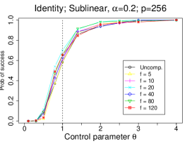
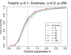
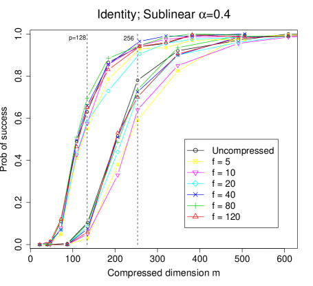
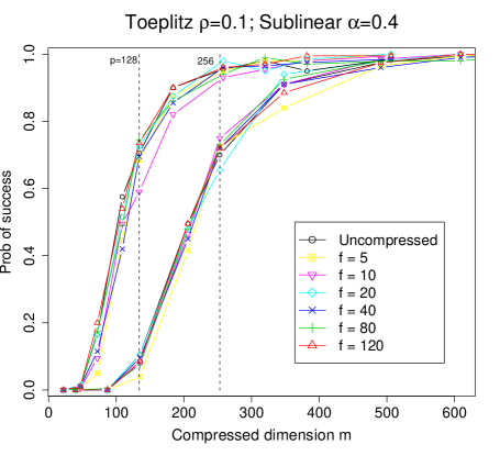
In this section we report the results of simulations designed to validate the theoretical analysis presented in the previous sections. We first present results that indicate the compressed lasso is comparable to the uncompressed lasso in recovering the sparsity pattern of the true linear model, in accordance with the analysis in Section 3. We then present experimental results on persistence that are in close agreement with the theoretical results of Section 4.

6.A Sparsistency

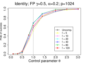
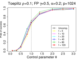
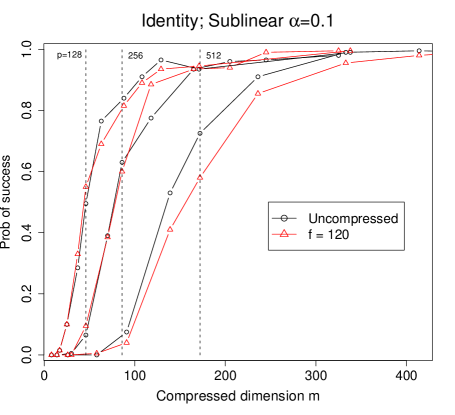
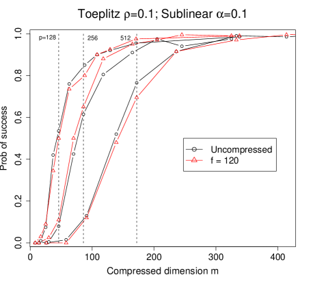
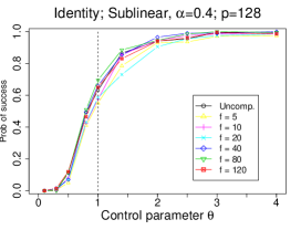
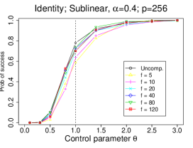
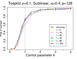
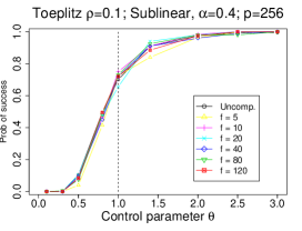
Here we run simulations to compare the compressed lasso with the uncompressed lasso in terms of the probability of success in recovering the sparsity pattern of $\beta^{*}$. We use random matrices for both $X$ and $\Phi$, and reproduce the experimental conditions shown in Wainwright (2006). A design parameter is the compression factor

$$f=\frac{n}{m}$$ (137)

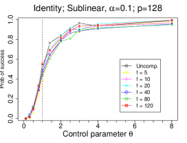
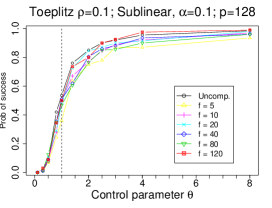
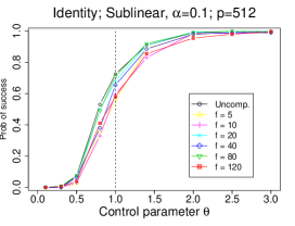
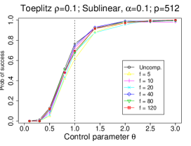
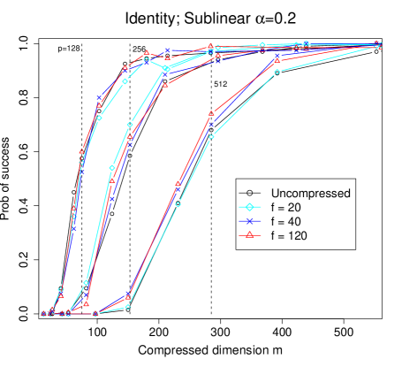
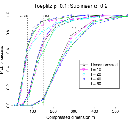
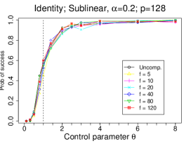
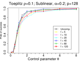
which indicates how much the original data are compressed. The results show that when the compression factor $f$ is large enough, the thresholding behaviors as specified in (19) and (20) for the uncompressed lasso carry over to the compressed lasso, when $X$ is drawn from a Gaussian ensemble. In general, the compression factor $f$ is well below the requirement that we have in Theorem 3.4 in case $X$ is deterministic.

In more detail, we consider the Gaussian ensemble for the projection matrix $\Phi$, where $\Phi_{i,j}\sim N(0,1/n)$ are independent. The noise vector is always composed of i.i.d. Gaussian random variables $\epsilon\sim N(0,\sigma^{2})$, where $\sigma^{2}=1$. We consider Gaussian ensembles for the design matrix $X$ with both diagonal and Toeplitz covariance. In the Toeplitz case, the covariance is given by

$$T(\rho) = \left[\begin{array}[]{cccccc}1&\rho&\rho^{2}&\ldots&\rho^{p-1}&\rho^{p-1}\\ \rho&1&\rho&\rho^{2}&\ldots&\rho^{p-2}\\ \rho^{2}&\rho&1&\rho&\ldots&\rho^{p-3}\\ \ldots&\ldots&\ldots&\ldots&\ldots&\ldots\\ \rho^{p-1}&\ldots&\rho^{3}&\rho^{2}&\rho&1\end{array}\right]_{p\times p}.$$ (143)

We use $\rho=0.1$. Both $I$ and $T(0.1)$ satisfy conditions (166a), (166b) and (168) (Zhao and Yu, 2007). For $\Sigma=I$, $\theta_{u}=\theta_{\ell}=1$, while for $\Sigma=T(0.1)$, $\theta_{u}\approx 1.84$ and $\theta_{\ell}\approx 0.46$ (Wainwright, 2006), for the uncompressed lasso in (19) and in (20).

In the following simulations, we carry out the lasso using procedure $\texttt{lars}(Y,X)$ that implements the LARS algorithm of Efron et al. (2004) to calculate the full regularization path; the parameter $\lambda$ is then selected along this path to match the appropriate condition specified by the analysis. For the uncompressed case, we run $\texttt{lars}(Y,X)$ such that

$$Y = X\beta^{*}+\epsilon,$$ (144)

and for the compressed case we run $\texttt{lars}(\Phi Y,\Phi X)$ such that

$$\Phi Y = \Phi X\beta^{*}+\Phi\epsilon.$$ (145)

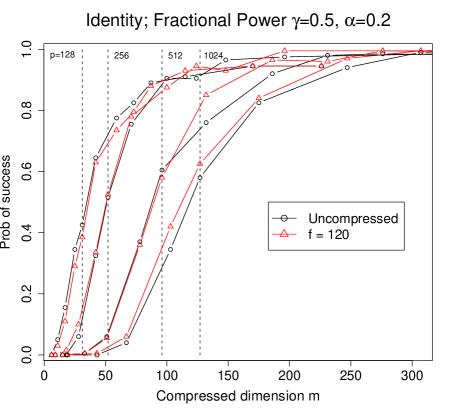
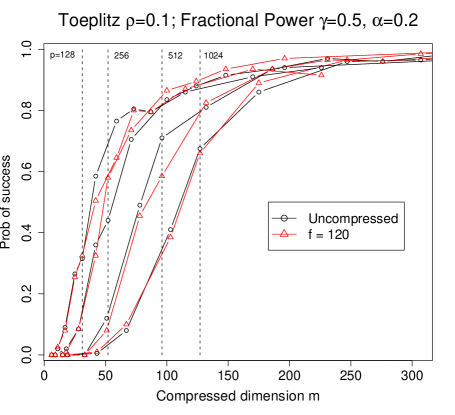
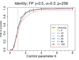
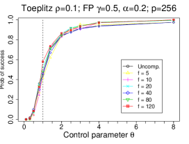
In each individual plot shown below, the covariance $\Sigma=\frac{1}{n}{\mathbb{E}}\left(X^{T}X\right)$ and model $\beta^{*}$ are fixed across all curves in the plot. For each curve, a compression factor $f\in\{5,10,20,40,80,120\}$ is chosen for the compressed lasso, and we show the probability of success for recovering the signs of $\beta^{*}$ as the number of compressed observations $m$ increases, where $m=2\theta\sigma^{2}s\log(p-s)+s+1$ for $\theta\in[0.1,u]$, for $u\geq 3$. Thus, the number of compressed observations is $m$, and the number of uncompressed observations is $n=fm$. Each point on a curve, for a particular $\theta$ or $m$, is an average over $200$ trials; for each trial, we randomly draw $X_{n\times p}$, $\Phi_{m\times n}$, and $\epsilon\in\mathbb{R}^{n}$. However $\beta^{*}$ remains the same for all $200$ trials, and is in fact fixed across different sets of experiments for the same sparsity level.

We consider two sparsity regimes:

Sublinear sparsity: $$s(p)=\frac{\alpha p}{\log(\alpha p)}\;\text{for $\alpha\in\{0.1,0.2,0.4\}$}$$ (146a)

Fractional power sparsity: $$s(p)=\alpha p^{\gamma}\;\text{for $\alpha=0.2$ and $\gamma=0.5$}.$$ (146b)

The coefficient vector $\beta^{*}$ is selected to be a prefix of a fixed vector

$$\beta^{\star}=(-0.9,-1.7,1.1,1.3,0.9,2,-1.7,-1.3,-0.9,-1.5,1.3,-0.9,1.3,1.1,0.9)^{T}$$ (147)

That is, if $s$ is the number of nonzero coefficients, then

$$\beta^{*}_{i}=\begin{cases}\beta^{\star}_{i}&\text{if $i\leq s$,}\\ 0&\text{otherwise}.\end{cases}$$ (148)

As an exception, for the case $s=2$, we set $\beta^{*}=(0.9,-1.7,0,\ldots,0)^{T}$.

After each trial, $\texttt{lars}(Y,X)$ outputs a “regularization path,” which is a set of estimated models ${\mathcal{P}}_{m}=\{\beta\}$ such that each $\beta\in{\mathcal{P}}_{m}$ is associated with a corresponding regularization parameter $\lambda(\beta)$, which is computed as

$$\lambda(\beta)=\frac{\left\lVert Y-X\widetilde{\beta}\right\rVert_{2}^{2}}{m\left\lVert\widetilde{\beta}\right\rVert_{1}}.$$ (149)

The coefficient vector $\widetilde{\beta}\in{\mathcal{P}}_{m}$ for which $\lambda(\widetilde{\beta})$ is closest to the value $\lambda_{m}$ is then evaluated for sign consistency, where

$$\lambda_{m}=c\sqrt{\frac{\log(p-s)\log s}{m}}.$$ (150)

If $\text{sgn}(\widetilde{\beta})=\text{sgn}(\beta^{*})$, the trial is considered a success, otherwise, it is a failure. We allow the constant $c$ that scales $\lambda_{m}$ to change with the experimental configuration (covariance $\Sigma$, compression factor $f$, dimension $p$ and sparsity $s$), but $c$ is a fixed constant across all $m$ along the same curve.

Table 1 summarizes the parameter settings that the simulations evaluate. In this table the ratio $m/p$ is for $m$ evaluated at $\theta=1$. The plots in Figures 1–4 show the empirical probability of the event ${\mathcal{E}}(\text{sgn}(\widetilde{\beta})=\text{sgn}(\beta^{*}))$ for each of these settings, which is a lower bound for that of the event $\{\mathop{\text{supp}\kern 0.86108pt}(\widetilde{\beta})=\mathop{\text{supp}\kern 0.86108pt}(\beta^{*})\}$. The figures clearly demonstrate that the compressed lasso recovers the true sparsity pattern as well as the uncompressed lasso.

	$\alpha$	$p=128$		$p=256$		$p=512$		$p=1024$
		$s(p)$	$m/p$	$s(p)$	$m/p$	$s(p)$	$m/p$	$s(p)$	$m/p$
Fractional Power	$0.2$	$2$	$0.24$	$3$	$0.20$	$5$	$0.19$	$6$	$0.12$
Sublinear	$0.1$	$3$	$0.36$	$5$	$0.33$	$9$	$0.34$
	$0.2$	$5$	$0.59$	$9$	$0.60$	$15$	$0.56$
	$0.4$	$9$	$1.05$	$15$	$1.00$

Table 1: Simulation parameters: $s(p)$ and ratio of $m/p$ for $\theta=1$ and $\sigma^{2}=1$.

Figure 1: Plots of the number of samples versus the probability of success. The four sets of curves on the left panel map to $p=128,256,512$ and $1024$, with dashed lines marking $m=2\theta s\log(p-s)+s+1$ for $\theta=1$ and $s=2,3,5$ and $6$ respectively. For clarity, the left plots only show the uncompressed lasso and the compressed lasso with $f=120$.

Figure 2: Plots of the number of samples versus the probability of success. The three sets of curves on the left panel map to $p=128,256$ and $512$ with dashed lines marking $m=2\theta s\log(p-s)+s+1$ for $\theta=1$ and $s=3,5$ and $9$ respectively.

Figure 3: Plots of the number of samples versus the probability of success. The three sets of curves on the left panel map to $p=128,256$ and $512$, with vertical dashed lines marking $m=2\theta s\log(p-s)+s+1$ for $\theta=1$, and $s=5,9$ and $15$ respectively.

Figure 4: Plots of the number of samples versus the probability of success. The two sets of curves on the left panel correspond to $p=128$ and $256$, with vertical dashed lines mapping to $m=2\theta s\log(p-s)+s+1$ for $\theta=1$, and $s=9$ and $15$ respectively.

6.B Persistence

We now study the behavior of predictive and empirical risks under compression. In this section, we refer to $\texttt{lasso2}(Y\sim X,L)$ as the code that solves the following $\ell_{1}$-constrained optimization problem directly, based on algorithms described by Osborne et al. (2000):

$$(P_{3})\hskip 28.45274pt\widetilde{\beta} = \mathop{\text{arg\,min}\kern 0.86108pt}\left\lVert Y-X\beta\right\rVert_{2}$$ (151a)

$$\text{such that }\left\lVert\beta\right\rVert_{1}\leq L.$$ (151b)

Let us first define the following $\ell_{1}$-balls ${B}_{n}$ and ${B}_{n,m}$ for a fixed uncompressed sample size $n$ and dimension $p_{n}$, and a varying compressed sample size $m$. By Greenshtein and Ritov (2004), given a sequence of sets of estimators

$${B}_{n}=\{\beta:\left\lVert\beta\right\rVert_{1}\leq L_{n}\},\;\text{where}\;L_{n}=\frac{n^{1/4}}{\sqrt{\log n}},$$ (152)

the uncompressed Lasso estimator $\widehat{\beta}_{n}$ as in (81) is persistent over ${B}_{n}$. Given $n,p_{n}$, Theorem 4.1 shows that, given a sequence of sets of estimators

$${B}_{n,m}=\{\beta:\left\lVert\beta\right\rVert_{1}\leq L_{n,m}\},\;\text{where}\;L_{n,m}=\frac{m^{1/4}}{\sqrt{\log(np_{n})}},$$ (153)

for $\log^{2}(np_{n})\leq m\leq n$, the compressed Lasso estimator $\widehat{\beta}_{n,m}$ as in (98) is persistent over ${B}_{n,m}$.

We use simulations to illustrate how close the compressed empirical risk computed through (162) is to that of the best compressed predictor $\beta_{*}$ as in (97) for a given set ${B}_{n,m}$, the size of which depends on the data dimension $n,p_{n}$ of an uncompressed design matrix $X$, and the compressed dimension $m$; we also illustrate how close these two type of risks are to that of the best uncompressed predictor defined in (80) for a given set ${B}_{n}$ for all $\log np_{n}\leq m\leq n$.

We let the row vectors of the design matrix be independent identical copies of a random vector $X\sim N(0,\Sigma)$. For simplicity, we generate $Y=X^{T}\beta^{*}+\epsilon$, where $X$ and $\beta^{*}\in\mathbb{R}^{p}$, ${\mathbb{E}}\left(\epsilon\right)=0$ and ${\mathbb{E}}\left(\epsilon^{2}\right)=\sigma^{2}$; note that ${\mathbb{E}}\left(Y|X\right)=X^{T}\beta^{*}$, although the persistence model need not assume this. Note that for all $m\leq n$,

$$L_{n,m}=\frac{m^{1/4}}{\sqrt{\log(np_{n})}}\leq L_{n}$$ (154)

Hence the risk of the model constructed on the compressed data over ${B}_{n,m}$ is necessarily no smaller than the risk of the model constructed on the uncompressed data over ${B}_{n}$, for all $m\leq n$.

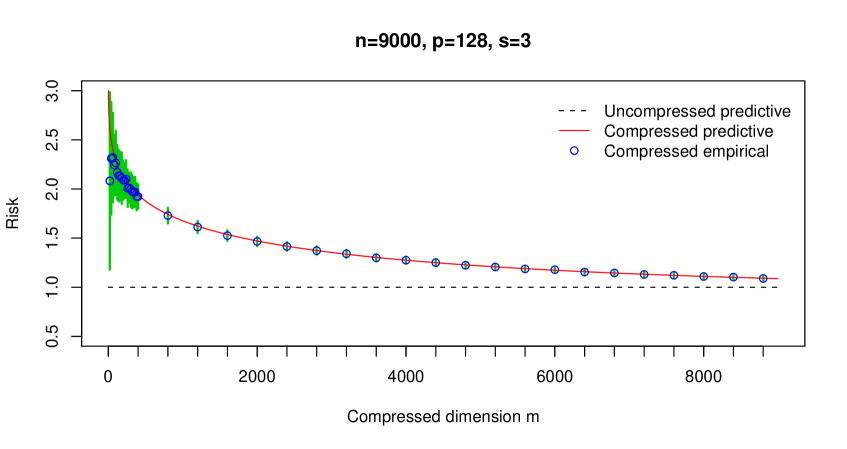
For $n=9000$ and $p=128$, we set $s(p)=3$ and $9$ respectively, following the sublinear sparisty (146a) with $\alpha=0.2$ and $0.4$; correspondingly, two set of coefficients are chosen for $\beta^{*}$,

$$\beta^{*}_{a} = (-0.9,1.1,0.687,0,\ldots,0)^{T}$$ (155)

so that $\left\lVert\beta^{*}\right\rVert_{1}<L_{n}$ and $\beta^{*}_{a}\in{B}_{n}$, and

$$\beta^{*}_{b} = (-0.9,-1.7,1.1,1.3,-0.5,2,-1.7,-1.3,-0.9,0,\ldots,0)^{T}$$ (156)

so that $\left\lVert\beta^{*}_{b}\right\rVert_{1}>L_{n}$ and $\beta^{*}_{b}\not\in{B}_{n}$.

In order to find $\beta_{*}$ that minimizes the predictive risk $R(\beta)={\mathbb{E}}\left((Y-X^{T}\beta)^{2}\right)$, we first derive the following expression for the risk. With $\Sigma=A^{T}A$, a simple calculation shows that

$${\mathbb{E}}(Y-X^{T}\beta)^{2}-{\mathbb{E}}(Y^{2}) = -\beta^{*T}\Sigma\beta^{*}+\left\lVert A\beta^{*}-A\beta\right\rVert_{2}^{2}.$$ (157)

Hence

$$R(\beta) = {\mathbb{E}}(Y^{2})-\beta^{*T}\Sigma\beta^{*}+\left\lVert A\beta^{*}-A\beta\right\rVert_{2}^{2}$$ (158a)

$$= {\mathbb{E}}(Y^{2})-\beta^{*T}{\mathbb{E}}\left(XX^{T}\right)\beta^{*}+\left\lVert A\beta^{*}-A\beta\right\rVert_{2}^{2}$$ (158b)

$$= \sigma^{2}+\left\lVert A\beta^{*}-A\beta\right\rVert_{2}^{2}.$$ (158c)

Figure 5: $L_{n}=2.6874$ for $n=9000$. Each data point corresponds to the mean empirical risk over $100$ trials, and each vertical bar shows one standard deviation. Top plot: risk versus compressed dimension for $\beta^{*}=\beta^{*}_{a}$; the uncompressed oracle predictive risk is $R=1$. Bottom plot: risk versus compressed dimension for $\beta^{*}=\beta^{*}_{b}$; the uncompressed oracle predictive risk is $R=9.81$.

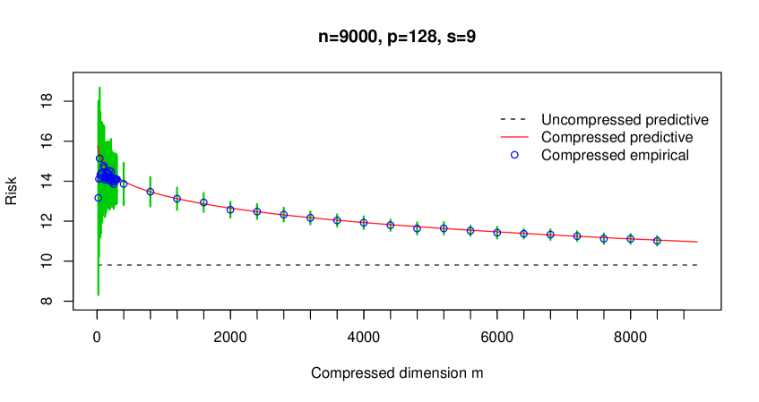For the next two sets of simulations, we fix $n=9000$ and $p_{n}=128$. To generate the uncompressed predictive (oracle) risk curve, we let

$$\widehat{\beta}_{n}=\mathop{\text{arg\,min}\kern 0.86108pt}_{\left\lVert\beta\right\rVert_{1}\leq L_{n}}R(\beta)=\mathop{\text{arg\,min}\kern 0.86108pt}_{\left\lVert\beta\right\rVert_{1}\leq L_{n}}\left\lVert A\beta^{*}-A\beta\right\rVert_{2}^{2}.$$ (159)

Hence we obtain $\beta_{*}$ by running $\texttt{lasso2}(\Sigma^{\frac{1}{2}}\beta^{*}\sim\Sigma^{\frac{1}{2}},L_{n})$. To generate the compressed predictive (oracle) curve, for each $m$, we let

$$\widehat{\beta}_{n,m}=\mathop{\text{arg\,min}\kern 0.86108pt}_{\left\lVert\beta\right\rVert_{1}\leq L_{n,m}}R(\beta)=\mathop{\text{arg\,min}\kern 0.86108pt}_{\left\lVert\beta\right\rVert_{1}\leq L_{n,m}}\left\lVert A\beta^{*}-A\beta\right\rVert_{2}^{2}.$$ (160)

Hence we obtain $\beta_{*}$ for each $m$ by running $\texttt{lasso2}(\Sigma^{\frac{1}{2}}\beta^{*}\sim\Sigma^{\frac{1}{2}},L_{n,m})$. We then compute oracle risk for both cases as

$$R(\widehat{\beta})=(\widehat{\beta}-\beta^{*})^{T}\Sigma(\widehat{\beta}-\beta^{*})+\sigma^{2}.$$ (161)

For each chosen value of $m$, we compute the corresponding empirical risk, its sample mean and sample standard deviation by averaging over $100$ trials. For each trial, we randomly draw $X_{n\times p}$ with independent row vectors $x_{i}\sim N(0,T(0.1))$, and $Y=X\beta^{*}+\epsilon$. If $\beta$ is the coefficient vector returned by $\texttt{lasso2}(\Phi Y\sim\Phi X,L_{n,m})$, then the empirical risk is computed as

$$\widehat{R}(\beta)=\gamma^{T}\widehat{\Sigma}\gamma,\;\;\text{where}\;\;\widehat{\Sigma}=\frac{1}{m}\mathbb{Q}^{T}\Phi^{T}\Phi\mathbb{Q}.$$ (162)

where $\mathbb{Q}_{n\times(p+1)}=[Y,X]$ and $\gamma=(-1,\beta_{1},\ldots,\beta_{p})$.

7 Proofs of Technical Results

7.A Connection to the Gaussian Ensemble Result

We first state a result which directly follows from the analysis of Theorem 3.4, and we then compare it with the Gaussian ensemble result of Wainwright (2006) that we summarized in Section 2.

First, let us state the following slightly relaxed conditions that are imposed on the design matrix by Wainwright (2006), and also by Zhao and Yu (2007), when $X$ is deterministic:

$$\left\|X^{T}_{S^{c}}X_{S}(X_{S}^{T}X_{S})^{-1}\right\|_{\infty} \leq 1-\eta,\;\;\text{for some $\eta\in(0,1]$, and}$$ (163a)

$$\Lambda_{\text{min}}\left({\textstyle\frac{1}{n}}X_{S}^{T}X_{S}\right) \geq C_{\text{min}}>0,$$ (163b)

where $\Lambda_{\text{min}}(A)$ is the smallest eigenvalue of $A$. In Section 7.B, Proposition 7.4 shows that $S$-incoherence implies the conditions in equations (163a) and (163b).

From the proof of Theorem 3.4 it is easy to verify the following. Let $X$ be a deterministic matrix satisfying conditions specified in Theorem 3.4, and let all constants be the same as in Theorem 3.4. Suppose that, before compression, we have noiseless responses $Y=X\beta^{*}$, and we observe, after compression, $\widetilde{X}=\Phi X$, and

$$\widetilde{Y}=\Phi Y+\epsilon=\widetilde{X}\beta^{*}+\epsilon,$$ (164)

where $\Phi_{m\times n}$ is a Gaussian ensemble with independent entries: $\Phi_{i,j}\sim N(0,1/n),\forall i,j$, and $\epsilon\sim N(0,\sigma^{2}I_{m})$. Suppose $m\geq\left(\frac{16C_{1}s^{2}}{\eta^{2}}+\frac{4C_{2}s}{\eta}\right)(\ln p+2\log n+\log 2(s+1))$ and $\lambda_{m}\rightarrow 0$ satisfies (37). Let $\widetilde{\beta}_{m}$ be an optimal solution to the compressed lasso, given $\widetilde{X},\widetilde{Y},\epsilon$ and $\lambda_{m}>0$:

$$\widetilde{\beta}_{m}=\mathop{\text{arg\,min}\kern 0.86108pt}_{\beta\in\mathbb{R}^{p}}\;\frac{1}{2m}\|\widetilde{Y}-\widetilde{X}\beta\|_{2}^{2}+\lambda_{m}\|\beta\|_{1}.$$ (165)

Then the compressed lasso is sparsistent: ${\mathbb{P}}\left(\mathop{\text{supp}\kern 0.86108pt}(\widetilde{\beta}_{m})=\mathop{\text{supp}\kern 0.86108pt}(\beta)\right)\rightarrow 1\;\;\text{as}\;m\rightarrow\infty$. Note that the upper bound on $m\leq\sqrt{\frac{n}{16\log n}}$ in (36) is no longer necessary, since we are handling the random vector $\epsilon$ with i.i.d entries rather than the non-i.i.d $\Phi\epsilon$ as in Theorem 3.4.

We first observe that the design matrix $\widetilde{X}=\Phi X$ as in (164) is exactly a Gaussian ensemble that Wainwright (2006) analyzes. Each row of $\widetilde{X}$ is chosen as an i.i.d. Gaussian random vector $\sim N(0,\Sigma)$ with covariance matrix $\Sigma={\textstyle\frac{1}{n}}X^{T}X$. In the following, let $\Lambda_{\min}(\Sigma_{SS})$ be the minimum eigenvalue of $\Sigma_{SS}$ and $\Lambda_{\max}(\Sigma)$ be the maximum eigenvalue of $\Sigma$. By imposing the $S$-incoherence condition on $X_{n\times p}$, we obtain the following two conditions on the covariance matrix $\Sigma$, which are required by Wainwright (2006) for deriving the threshold conditions (19) and (20), when the design matrix is a Gaussian ensemble like $\widetilde{X}$:

$$\left\lVert\Sigma_{{S^{c}}S}(\Sigma_{SS})^{-1}\right\rVert_{\infty} \leq 1-\eta,\;\;\text{for $\eta\in(0,1]$, and}$$ (166a)

$$\Lambda_{\min}(\Sigma_{SS}) \geq C_{\text{min}}>0.$$ (166b)

When we apply this to $\widetilde{X}=\Phi X$ where $\Phi$ is from the Gaussian ensemble and $X$ is deterministic, this condition requires that

$$\left\lVert X_{S^{c}}^{T}X_{S}(X_{S}^{T}X_{S})^{-1}\right\rVert_{\infty} \leq 1-\eta,\;\;\text{for $\eta\in(0,1]$, and}$$ (167a)

$$\Lambda_{\text{min}}\left({\textstyle\frac{1}{n}}X_{S}^{T}X_{S}\right) \geq C_{\text{min}}>0.$$ (167b)

since in this case ${\mathbb{E}}\left({\textstyle\frac{1}{m}}X^{T}\Phi^{T}\Phi X\right)={\textstyle\frac{1}{n}}X^{T}X$. In addition, it is assumed in Wainwright (2006) that there exists a constant $C_{\max}$ such that

$$\Lambda_{\text{max}}(\Sigma)\leq C_{\max}.$$ (168)

This condition need not hold for ${\textstyle\frac{1}{n}}X^{T}X$; In more detail, given $\Lambda_{\text{max}}({\textstyle\frac{1}{n}}X^{T}X)=\frac{1}{n}\Lambda_{\text{max}}(X^{T}X)=\frac{1}{n}\left\lVert X\right\rVert_{2}^{2}$, we first obtain a loose upper and lower bound for $\left\lVert X\right\rVert_{2}^{2}$ through the Frobenius norm $\left\lVert X\right\rVert_{F}$ of $X$. Given that $\left\lVert X_{j}\right\rVert_{2}^{2}=n,\forall j\in\{1,\ldots,p\}$, we have $\left\lVert X\right\rVert^{2}_{F}=\sum_{j=1}^{p}\sum_{i=1}^{n}|X_{ij}|^{2}=pn$. Thus by $\left\lVert X\right\rVert_{2}\leq\left\lVert X\right\rVert_{F}\leq\sqrt{p}\left\lVert X\right\rVert_{2}$, we obtain

$$n=\frac{1}{p}\left\lVert X\right\rVert^{2}_{F}\leq\left\lVert X\right\rVert_{2}^{2}\leq\left\lVert X\right\rVert^{2}_{F}=pn,$$ (169)

which implies that $1\leq\Lambda_{\max}({\textstyle\frac{1}{n}}X^{T}X)\leq p$. Since we allow $p$ to grow with $n$, (168) need not hold.

Finally we note that the conditions on $\lambda_{m}$ in the Gaussian Ensemble result of Wainwright (2006) are (37 $a$) and a slight variation of (37 $b$):

$$\displaystyle\frac{1}{\rho_{m}}\left\{\sqrt{\frac{\log s}{m}}+\lambda_{m}\right\}\rightarrow 0;$$ (170)

hence if we further assume that $\left\lVert({\textstyle\frac{1}{n}}X_{S}^{T}X_{S})^{-1}\right\rVert_{\infty}\leq D_{\max}$ for some constant $D_{\max}\leq+\infty$, as required by Wainwright (2006) on $\left\lVert\Sigma_{SS}^{-1}\right\rVert_{\infty}$,  (37 $b$) and (170) are equivalent.

Hence by imposing the $S$-incoherence condition on a deterministic $X_{n\times p}$ with all columns of $X$ having $\ell_{2}$-norm $n$, when $m$ satisfies the lower bound in (36), rather than (19) with $\theta_{u}=\frac{C_{\max}}{\eta^{2}C_{\min}}$ with $C_{\max}$ as in (168), we have shown that the probability of sparsity recovery through lasso approaches one, given $\lambda_{m}$ satisfies (37), when the design matrix is a Gaussian Ensemble generated through $\Phi X$ with $\Phi_{m\times n}$ having independent $\Phi_{i,j}\in N(0,1/n),\forall i,j$. We do not have a comparable result for the failure of recovery given (20).

7.B $S$-Incoherence

We first state some generally useful results about matrix norms.

Theorem 7.1

.  (Horn and Johnson, 1990, p. 301) If $|\kern-0.86108pt|\kern-0.86108pt|\cdot|\kern-0.86108pt|\kern-0.86108pt|$ is a matrix norm and $|\kern-0.86108pt|\kern-0.86108pt|A|\kern-0.86108pt|\kern-0.86108pt|<1$, then $I+A$ is invertible and

$$(I+A)^{-1}=\sum_{k=0}^{\infty}(-A)^{k}.$$ (171)

Proposition 7.2

.  If the matrix norm $\left\lVert\cdot\right\rVert$ has the property that $\left\lVert I\right\rVert=1$, and if $A\in M_{n}$ is such that $\left\lVert A\right\rVert<1$, we have

$$\frac{1}{1+\left\lVert A\right\rVert}\leq\left\lVert(I+A)^{-1}\right\rVert\leq\frac{1}{1-\left\lVert A\right\rVert}.$$ (172)

Proof.   The upper bound follows from Theorem 7.1 and triangle-inequality;

$$\left\lVert(I+A)^{-1}\right\rVert=\left\lVert\sum_{k=0}^{\infty}(-A)^{k}\right\rVert\leq\sum_{k=0}^{\infty}\left\lVert-A\right\rVert^{k}=\sum_{k=0}^{\infty}\left\lVert A\right\rVert^{k}=\frac{1}{1-\left\lVert A\right\rVert}.$$ (173)

The lower bound follows that general inequality $\left\lVert B^{-1}\right\rVert\geq\frac{1}{\left\lVert B\right\rVert}$, given that $\left\lVert I\right\rVert\leq\left\lVert B\right\rVert\left\lVert B^{-1}\right\rVert$ and the triangle inequality: $\left\lVert A+I\right\rVert\leq\left\lVert A\right\rVert+\left\lVert I\right\rVert=\left\lVert A\right\rVert+1$.

$$\left\lVert(A+I)^{-1}\right\rVert\geq\frac{1}{\left\lVert A+I\right\rVert}\geq\frac{1}{1+\left\lVert A\right\rVert}$$ (174)

$\;\;\scriptstyle\Box$

Let us define the following symmetric matrices, that we use throughout the rest of this section.

$$A = \frac{1}{n}X_{S}^{T}X_{S}-I_{\left|S\right|}$$ (175a)

$$\widetilde{A} = \frac{1}{m}(\Phi X)_{S}^{T}(\Phi X)_{S}-I_{s}=\frac{1}{m}Z_{S}^{T}Z_{S}-I_{s}.$$ (175b)

We next show the following consequence of the $S$-Incoherence condition.

Proposition 7.3

.  Let $X$ be an $n\times p$ that satisfies the $S$-Incoherence condition. Then for the symmetric matrix $A$ in 175a , we have $\left\lVert A\right\rVert_{\infty}=\left\lVert A\right\rVert_{1}\leq 1-\eta$, for some $\eta\in(0,1]$, and

$$\left\lVert A\right\rVert_{2}\leq\sqrt{\left\lVert A\right\rVert_{\infty}\left\lVert A\right\rVert_{1}}\leq 1-\eta.$$ (176)

and hence $\Lambda_{\min}(\frac{1}{n}X^{T}_{S}X_{S})\geq\eta$, i.e., the $S$-Incoherence condition implies condition (163b).

Proof.   Given that $\left\lVert A\right\rVert_{2}<1$, $\left\lVert I\right\rVert_{2}=1$, and by Proposition 7.2,

$$\Lambda_{\min}(\frac{1}{n}X^{T}_{S}X_{S})=\frac{1}{\left\lVert(\frac{1}{n}X^{T}_{S}X_{S})^{-1}\right\rVert_{2}}=\frac{1}{\left\lVert(I+A)^{-1}\right\rVert_{2}}\geq 1-\left\lVert A\right\rVert_{2}\geq\eta>0$$ (177)

$\;\;\scriptstyle\Box$

Proposition 7.4

.  The $S$-Incoherence condition on an $n\times p$ matrix $X$ implies conditions  (163a) and (163b).

Proof.   It remains to show (163a) given Proposition 7.3. Now suppose that the incoherence condition holds for some $\eta\in(0,1]$, i.e.,$\left\lVert\frac{1}{n}X_{S^{c}}^{T}X_{S}\right\rVert_{\infty}+\left\lVert A\right\rVert_{\infty}\leq 1-\eta$, we must have

$$\frac{\left\lVert\frac{1}{n}X_{S^{c}}^{T}X_{S}\right\rVert_{\infty}}{1-\left\lVert A\right\rVert_{\infty}}\leq 1-\eta,$$ (178)

given that $\left\lVert\frac{1}{n}X_{S^{c}}^{T}X_{S}\right\rVert_{\infty}+\left\lVert A\right\rVert_{\infty}(1-\eta)\leq 1-\eta$ and $1-\left\lVert A\right\rVert_{\infty}\geq\eta>0$.

Next observe that, given $\left\lVert A\right\rVert_{\infty}<1$, by Proposition 7.2

$$\left\lVert(\frac{1}{n}X_{S}^{T}X_{S})^{-1}\right\rVert_{\infty}=\left\lVert(I+A)^{-1}\right\rVert_{\infty}\leq\frac{1}{1-\left\lVert A\right\rVert_{\infty}}.$$ (179)

Finally, we have

$$\left\lVert X_{S^{c}}^{T}X_{S}(X_{S}^{T}X_{S})^{-1}\right\rVert_{\infty} \leq \left\lVert\frac{1}{n}X_{S^{c}}^{T}X_{S}\right\rVert_{\infty}\left\lVert(\frac{1}{n}X_{S}^{T}X_{S})^{-1}\right\rVert_{\infty}$$ (180a)

$$\leq \frac{\left\lVert\frac{1}{n}X_{S^{c}}^{T}X_{S}\right\rVert_{\infty}}{1-\left\lVert A\right\rVert_{\infty}}\leq 1-\eta.$$ (180b)

$\;\;\scriptstyle\Box$

7.C Proof of Lemma 3.5

Let $\Phi_{ij}=\frac{1}{\sqrt{n}}g_{ij}$, where $g_{ij},\forall i=1,\ldots,m,j=1,\ldots,n$ are independent $N(0,1)$ random variables. We define

$$Y_{\ell}:=\sum_{k=1}^{n}\sum_{j=1}^{n}g_{\ell,k}g_{\ell,j}x_{k}y_{j},$$ (181)

and we thus have the following:

$$\left\langle\Phi x,\Phi y\right\rangle = \frac{1}{n}\sum_{\ell=1}^{m}\sum_{k=1}^{n}\sum_{j=1}^{n}g_{\ell,k}g_{\ell,j}x_{k}y_{j}$$ (182a)

$$= \frac{1}{n}\sum_{\ell=1}^{m}Y_{\ell},$$ (182b)

where $Y_{\ell},\forall\ell$, are independent random variables, and

$${\mathbb{E}}\left(Y_{\ell}\right) = {\mathbb{E}}\left(\sum_{k=1}^{n}\sum_{j=1}^{n}g_{\ell,k}g_{\ell,j}x_{k}y_{j}\right)$$ (183a)

$$= \sum_{k=1}^{n}x_{k}y_{k}{\mathbb{E}}\left(g_{\ell,k}^{2}\right)$$ (183b)

$$= \left\langle x,y\right\rangle$$ (183c)

Let us define a set of zero-mean independent random variables $Z_{1},\ldots,Z_{m}$,

$$Z_{\ell}:=Y_{\ell}-\left\langle x,y\right\rangle=Y_{\ell}-{\mathbb{E}}\left(Y_{\ell}\right),$$ (184)

such that

$$\frac{n}{m}\left\langle\Phi x,\Phi y\right\rangle-\left\langle x,y\right\rangle = \frac{1}{m}\sum_{\ell=1}^{m}Y_{\ell}-\left\langle x,y\right\rangle$$ (185a)

$$= \frac{1}{m}\sum_{\ell=1}^{m}(Y_{\ell}-\left\langle x,y\right\rangle)$$ (185b)

$$= \frac{1}{m}\sum_{\ell=1}^{m}Z_{\ell}.$$ (185c)

In the following, we analyze the integrability and tail behavior of $Z_{\ell},\forall\ell$, which is known as “Gaussian chaos” of order $2$.

We first simplify notation by defining $Y:=\sum_{k=1}^{n}\sum_{j=1}^{n}g_{k}g_{j}x_{k}y_{j}$, where $g_{k},g_{j}$ are independent $N(0,1)$ variates, and $Z$,

$$Z:=Y-{\mathbb{E}}\left(Y\right)=\sum_{k=1}^{n}\sum_{j=1,j\not=k}^{n}g_{k}g_{j}x_{k}y_{j}+\sum_{k=1}^{n}(g_{k}^{2}-1)x_{k}y_{k},$$ (186)

where ${\mathbb{E}}\left(Z\right)=0$. Applying a general bound of Ledoux and Talagrand (1991) for Gaussian chaos gives that

$${\mathbb{E}}\left(\left\lvert Z\right\rvert^{q}\right)\leq(q-1)^{q}({\mathbb{E}}\left(\left\lvert Z\right\rvert^{2}\right))^{q/2}$$ (187)

for all $q>2$.

The following claim is based on (187), whose proof appears in Rauhut et al. (2007), which we omit.

Claim 7.5

.  (Rauhut et al. (2007)) Let $M=e({\mathbb{E}}\left(|Z|^{2}\right)^{1/2}$ and $s=\frac{2e}{\sqrt{6\pi}}{\mathbb{E}}\left(\left\lvert Z\right\rvert^{2}\right)$.

$$\forall q>2,\;\;{\mathbb{E}}\left(Z^{q}\right)\leq q!M^{q-2}s/2.$$

Clearly the above claim holds for $q=2$, since trivially ${\mathbb{E}}\left(\left\lvert Z\right\rvert^{q}\right)\leq q!M^{q-2}s/2$ given that for $q=2$

$$q!M^{q-2}s/2 = 2M^{2-2}s/2=s$$ (188a)

$$= \frac{2e}{\sqrt{6\pi}}{\mathbb{E}}\left(\left\lvert Z\right\rvert^{2}\right)\approx 1.2522{\mathbb{E}}\left(\left\lvert Z\right\rvert^{2}\right).$$ (188b)

Finally, let us determine ${\mathbb{E}}\left(\left\lvert Z\right\rvert^{2}\right)$.

$${\mathbb{E}}\left(\left\lvert Z\right\rvert^{2}\right) = {\mathbb{E}}\left(\left(\sum_{k=1}^{n}\sum_{j=1,j\not=k}^{n}g_{k}g_{j}x_{k}y_{j}++\sum_{k=1}^{n}(g_{k}^{2}-1)x_{k}y_{k}\right)^{2}\right)$$ (189a)

$$= \sum_{k\not=j}{\mathbb{E}}\left(g_{j}^{2}\right){\mathbb{E}}\left(g_{k}^{2}\right)x_{j}^{2}y_{k}^{2}+\sum_{k=1}^{n}{\mathbb{E}}\left(g_{k}^{2}-1\right)x_{k}^{2}y_{k}^{2}$$ (189b)

$$= \sum_{k\not=j}x_{j}^{2}y_{k}^{2}+2\sum_{k=1}^{n}x_{k}^{2}y_{k}^{2}$$ (189c)

$$\leq 2\left\lVert x\right\rVert_{2}^{2}\left\lVert y\right\rVert_{2}^{2}$$ (189d)

$$\leq 2,$$ (189e)

given that $\left\lVert x\right\rVert_{2},\left\lVert y\right\rVert_{2}\leq 1$.

Thus for independent random variables $Z_{i},\forall i=1,\ldots,m$, we have

$${\mathbb{E}}\left(Z_{i}^{q}\right)\leq q!M^{q-2}v_{i}/2,$$ (190)

where $M=e({\mathbb{E}}\left(|Z|^{2}\right)^{1/2}\leq e\sqrt{2}$ and $v_{i}=\frac{2e}{\sqrt{6\pi}}{\mathbb{E}}\left(\left\lvert Z\right\rvert^{2}\right)\leq\frac{4e}{\sqrt{6\pi}}\leq 2.5044,\forall i$.

Finally, we apply the following theorem, the proof of which follows arguments from Bennett (1962):

Theorem 7.6

. (Bennett Inequality (Bennett, 1962)) Let $Z_{1},\ldots,Z_{m}$ be independent random variables with zero mean such that

$${\mathbb{E}}\left(\left\lvert Z_{i}\right\rvert^{q}\right)\leq q!M^{q-2}v_{i}/2,$$ (191)

for every $q\geq 2$ and some constant $M$ and $v_{i},\forall i=1,\ldots,m$. Then for $x>0$,

$${\mathbb{P}}\left(\left\lvert\sum_{i=1}^{m}\left\lvert Z_{i}\right\rvert\right\rvert\geq\tau\right)\leq 2\exp\left(-\frac{\tau^{2}}{v+M\tau}\right)$$ (192)

with $v=\sum_{i=1}^{m}v_{i}$.

We can then apply the Bennett Inequality to obtain the following:

$${\mathbb{P}}\left(\left\lvert\frac{n}{m}\left\langle\Phi x,\Phi y\right\rangle-\left\langle x,y\right\rangle\right\rvert\geq\tau\right) = {\mathbb{P}}\left(\left\lvert\frac{1}{m}\sum_{\ell=1}^{m}Z_{\ell}\right\rvert\geq\tau\right)$$ (193a)

$$= {\mathbb{P}}\left(\left\lvert\sum_{\ell=1}^{m}Z_{\ell}\right\rvert\geq m\tau\right)$$ (193b)

$$\leq 2\exp\left(-\frac{(m\tau)^{2}}{2\sum_{i=1}^{m}v_{i}+2Mm\tau}\right)$$ (193c)

$$= 2\exp\left(-\frac{m\tau^{2}}{2/m\sum_{i=1}^{m}v_{i}+2M\tau}\right)$$ (193d)

$$\leq 2\exp\left(-\frac{m\tau^{2}}{C_{1}+C_{2}\tau}\right)$$ (193e)

with $C_{1}=\frac{4e}{\sqrt{6\pi}}\approx 2.5044$ and $C_{2}=\sqrt{8e}\approx 7.6885$.  $\;\;\scriptstyle\Box$

7.D Proof of Proposition 3.6

We use Lemma 3.5, except that we now have to consider the change in absolute row sums of $\left\lVert\frac{1}{n}X_{S^{c}}^{T}X_{S}\right\rVert_{\infty}$ and $\left\lVert A\right\rVert_{\infty}$ after multiplication by $\Phi$. We first prove the following claim.

Claim 7.7

.  Let $X$ be a deterministic matrix that satisfies the incoherence condition. If

$$\left\lvert\frac{1}{m}\left\langle\Phi X_{i},\Phi X_{j}\right\rangle-\frac{1}{n}\left\langle X_{i},X_{j}\right\rangle\right\rvert\leq\tau,$$ (194)

for any two columns $X_{i},X_{j}$ of $X$ that are involved in (45b), then

$$\left\lVert\frac{1}{m}(\Phi X)_{S^{c}}^{T}(\Phi X)_{S}\right\rVert_{\infty}+\left\lVert\widetilde{A}\right\rVert_{\infty}\leq 1-\eta+2s\tau,$$ (195)

and

$$\Lambda_{\min}\left({\textstyle\frac{1}{m}}Z^{T}_{S}Z_{S}\right)\geq\eta-s\tau.$$ (196)

Proof.   It is straightforward to show (195). Since each row in $\frac{1}{m}(\Phi X)_{S^{c}}^{T}(\Phi X)_{S}$ and $A$ has $s$ entries, where each entry changes by at most $\tau$ compared to those in $\frac{1}{n}X^{T}X$, the absolute sum of any row can change by at most $s\tau$,

$$\left\lvert\left\lVert\frac{1}{m}(\Phi X)_{S^{c}}^{T}(\Phi X)_{S}\right\rVert_{\infty}-\left\lVert\frac{1}{n}X_{S^{c}}^{T}X_{S}\right\rVert_{\infty}\right\rvert \leq s\tau,$$ (197a)

$$\left\lvert\left\lVert\widetilde{A}\right\rVert_{\infty}-\left\lVert A\right\rVert_{\infty}\right\rvert \leq s\tau,$$ (197b)

and hence

$$\left\lVert\frac{1}{m}(\Phi X)_{S^{c}}^{T}(\Phi X)_{S}\right\rVert_{\infty}+\left\lVert\widetilde{A}\right\rVert_{\infty} \leq \left\lVert\frac{1}{n}X_{S^{c}}^{T}X_{S}\right\rVert_{\infty}+\left\lVert A\right\rVert_{\infty}+2s\tau$$ (198a)

$$\leq 1-\eta+2s\tau.$$ (198b)

We now prove (196). Defining $E=\widetilde{A}-A$, we have

$$\left\lVert E\right\rVert_{2}\leq s\max_{i,j}|\widetilde{A}_{i,j}-A_{i,j}|\leq s\tau,$$ (199)

given that each entry of $\widetilde{A}$ deviates from that of $A$ by at most $\tau$. Thus we have that

$$\left\lVert\widetilde{A}\right\rVert_{2} = \left\lVert A+E\right\rVert_{2}$$ (200a)

$$\leq \left\lVert A\right\rVert_{2}+\left\lVert E\right\rVert_{2}$$ (200b)

$$\leq \left\lVert A\right\rVert_{2}+s\max_{i,j}|E_{i,j}|$$ (200c)

$$\leq 1-\eta+s\tau,$$ (200d)

where $\left\lVert A\right\rVert_{2}\leq 1-\eta$ is due to Proposition 7.3.

Given that $\left\lVert I\right\rVert_{2}=1$ and $\left\lVert A\right\rVert_{2}<1$, by Proposition 7.2

$$\Lambda_{\min}\left({\textstyle\frac{1}{m}}Z^{T}_{S}Z_{S}\right) = \frac{1}{\left\lVert(\frac{1}{m}Z^{T}_{S}Z_{S})^{-1}\right\rVert_{2}}$$ (201a)

$$= \frac{1}{\left\lVert(I+\widetilde{A})^{-1}\right\rVert_{2}}$$ (201b)

$$\geq 1-\left\lVert\widetilde{A}\right\rVert_{2}$$ (201c)

$$\geq \eta-s\tau.$$ (201d)

$\;\;\scriptstyle\Box$

We let ${\mathcal{E}}$ represents union of the following events, where $\tau=\frac{\eta}{4s}$:

1. $\exists i\in S,j\in S^{c}$, such that $\left\lvert\frac{1}{m}\left\langle\Phi X_{i},\Phi X_{j}\right\rangle-\frac{1}{n}\left\langle X_{i},X_{j}\right\rangle\right\rvert\geq\tau$,

2. $\exists i,i^{\prime}\in S$, such that $\left\lvert\frac{1}{m}\left\langle\Phi X_{i},\Phi X_{i^{\prime}}\right\rangle-\frac{1}{n}\left\langle X_{i},X_{i^{\prime}}\right\rangle\right\rvert\geq\tau$,

3. $\exists j\in S^{c}$, such that

   $$\left\lvert\frac{1}{m}\left\langle\Phi X_{j},\Phi X_{j}\right\rangle-\frac{1}{n}\left\langle X_{j},X_{j}\right\rangle\right\rvert = \left\lvert\frac{1}{m}\left\lVert\Phi X_{j}\right\rVert_{2}^{2}-\frac{1}{n}\left\lVert X_{j}\right\rVert_{2}^{2}\right\rvert$$ (202a)

   $$> \tau.$$ (202b)

Consider first the implication of ${\mathcal{E}}^{c}$, i.e., when none of the events in ${\mathcal{E}}$ happens. We immediately have that  (45b), (196) and (46b) all simultaneously hold by Claim 7.7; and  (45b) implies that the incoherence condition is satisfied for $Z=\Phi X$ by Proposition 7.4.

We first bound the probability of a single event counted in ${\mathcal{E}}$. Consider two column vectors $x=\frac{X_{i}}{\sqrt{n}},y=\frac{X_{j}}{\sqrt{n}}\in\mathbb{R}^{n}$ in matrix $\frac{X}{\sqrt{n}}$, we have $\left\lVert x\right\rVert_{2}=1,\left\lVert y\right\rVert_{2}=1$, and

$${\mathbb{P}}\left(\left\lvert\frac{1}{m}\left\langle\Phi X_{i},\Phi X_{j}\right\rangle-\frac{1}{n}\left\langle X_{i},X_{j}\right\rangle\right\rvert\geq\tau\right)$$ (203a)

$$= {\mathbb{P}}\left(\left\lvert\frac{n}{m}\left\langle\Phi x,\Phi y\right\rangle-\left\langle x,y\right\rangle\right\rvert\geq\tau\right)\leq 2\exp\left(\frac{-m\tau^{2}}{C_{1}+C_{2}\tau}\right)$$ (203b)

$$\leq 2\exp\left(-\frac{m\eta^{2}/16s^{2}}{C_{1}+C_{2}\eta/4s}\right)$$ (203c)

given that $\tau=\frac{\eta}{4s}$.

We can now bound the probability that any such large-deviation event happens. Recall that $p$ is the total number of columns of $X$ and $s=\left|S\right|$; the total number of events in ${\mathcal{E}}$ is less than $p(s+1)$. Thus

$${\mathbb{P}}\left({\mathcal{E}}\right) \leq p(s+1){\mathbb{P}}\left(\left\lvert\frac{1}{m}\left\langle\Phi X_{i},\Phi X_{j}\right\rangle-\frac{1}{n}\left\langle X_{i},X_{j}\right\rangle\right\rvert\geq\frac{\eta}{4s}\right)$$ (204a)

$$\leq 2p(s+1)\exp\left(-\frac{m\eta^{2}/16s^{2}}{C_{1}+C_{2}\eta/4s}\right)$$ (204b)

$$= 2p(s+1)\exp\left(-(\ln p+c\ln n+\ln 2(s+1))\right)\leq\frac{1}{n^{c}},$$ (204c)

given that $m\geq\left(\frac{16C_{1}s^{2}}{\eta^{2}}+\frac{4C_{2}s}{\eta}\right)(\ln p+c\ln n+\ln 2(s+1))$.  $\;\;\scriptstyle\Box$

7.E Proof of Theorem 3.7

We first show that each of the diagonal entries of $\Phi\Phi^{T}$ is close to its expected value.

We begin by stating state a deviation bound for the $\chi^{2}_{n}$ distribution in Lemma 7.8 and its corollary, from which we will eventually derive a bound on $|R_{i,i}|$. Recall that the random variable $Q\sim\chi^{2}_{n}$ is distributed according to the chi-square distribution if $Q=\sum_{i=1}^{n}Y^{2}_{i}$ with $Y_{i}\sim N(0,1)$ that are independent and normally distributed.

Lemma 7.8

.  (Johnstone (2001))

$${\mathbb{P}}\left(\frac{\chi^{2}_{n}}{n}-1<-\epsilon\right) \leq \exp\left(\frac{-n\epsilon^{2}}{4}\right),\;\text{for}\;0\leq\epsilon\leq 1,$$ (205a)

$${\mathbb{P}}\left(\frac{\chi^{2}_{n}}{n}-1>\epsilon\right) \leq \exp\left(\frac{-3n\epsilon^{2}}{16}\right),\;\text{for}\;0\leq\epsilon\leq\frac{1}{2}.$$ (205b)

Corollary 7.9

. (Deviation Bound for Diagonal Entries of $\Phi\Phi^{T}$) Given a set of independent normally distributed random variables $X_{1},\ldots,X_{n}\sim N(0,\sigma^{2}_{X})$, for $0\leq\epsilon<\frac{1}{2}$,

$${\mathbb{P}}\left(\left|\frac{1}{n}\sum_{i=1}^{n}X^{2}_{i}-\sigma^{2}_{X}\right|>\epsilon\right)\leq\exp\left(\frac{-n\epsilon^{2}}{4\sigma_{X}^{4}}\right)+\exp\left(\frac{-3n\epsilon^{2}}{16\sigma_{X}^{4}}\right).$$ (206)

Proof.   Given that $X_{1},\ldots,X_{n}\sim N(0,\sigma^{2}_{X})$, we have $\frac{X_{i}}{\sigma_{X}}\sim N(0,1)$, and

$$\sum_{i=1}^{n}\left(\frac{X_{i}}{\sigma_{X}}\right)^{2}\sim\chi^{2}_{n},$$ (207)

Thus by Lemma 7.8, we obtain the following:

$${\mathbb{P}}\left(\frac{1}{n}{\sum_{i=1}^{n}\frac{X^{2}_{i}}{\sigma^{2}_{X}}}-1<-\epsilon\right) \leq \exp\left(\frac{-n\epsilon^{2}}{4}\right),\;0\leq\epsilon\leq 1$$ (208a)

$${\mathbb{P}}\left(\frac{1}{n}{\sum_{i=1}^{n}\frac{X^{2}_{i}}{\sigma^{2}_{X}}}-1>\epsilon\right) \leq \exp\left(\frac{-3n\epsilon^{2}}{16}\right),\;0\leq\epsilon\leq\frac{1}{2}.$$ (208b)

Therefore we have the following by a union bound, for $\epsilon<\frac{1}{2}$,

$${\mathbb{P}}\left(\left|\frac{1}{n}\sum_{i=1}^{n}X^{2}_{i}-\sigma^{2}_{X}\right|>\epsilon\right)\leq$$ (209b)

$${\mathbb{P}}\left(\sigma^{2}_{X}\left(\frac{\chi^{2}_{n}}{n}-1\right)<-\epsilon\right)+{\mathbb{P}}\left(\sigma^{2}_{X}\left(\frac{\chi^{2}_{n}}{n}-1\right)>\epsilon\right)$$

$$\leq {\mathbb{P}}\left(\frac{\chi^{2}_{n}}{n}-1<-\frac{\epsilon}{\sigma^{2}_{X}}\right)+{\mathbb{P}}\left(\frac{\chi^{2}_{n}}{n}-1>\frac{\epsilon}{\sigma^{2}_{X}}\right)$$ (209c)

$$\leq \exp\left(\frac{-n\epsilon^{2}}{4\sigma_{X}^{4}}\right)+\exp\left(\frac{-3n\epsilon^{2}}{16\sigma_{X}^{4}}\right).$$ (209e)

$\;\;\scriptstyle\Box$

We next show that the non-diagonal entries of $\Phi\Phi^{T}$ are close to zero, their expected value.

Lemma 7.10

.  (Johnstone (2001)) Given independent random variables $X_{1},\ldots,X_{n}$, where $X_{1}=z_{1}z_{2}$, with $z_{1}$ and $z_{2}$ being independent $N(0,1)$ variables,

$${\mathbb{P}}\left(\frac{1}{n}\sum_{i=1}^{n}X_{i}>\sqrt{\frac{b\log n}{n}}\right) \leq Cn^{-3b/2}.$$ (210)

Corollary 7.11

.  (Deviation Bound for Non-Diagonal Entries of $\Phi\Phi^{T}$) Given a collection of i.i.d. random variables $Y_{1},\ldots,Y_{n}$, where $Y_{i}=x_{1}x_{2}$ is a product of two independent normal random variables $x_{1},x_{2}\sim N(0,\sigma^{2}_{X})$, we have

$${\mathbb{P}}\left(\left|\frac{1}{n}\sum_{i=1}^{n}Y_{i}\right|>\sqrt{\frac{A\log n}{n}}\right)\;\leq\;2Cn^{-3A/2\sigma_{X}^{4}}.$$ (211)

Proof.   First, we let

$$X_{i}=\frac{Y_{i}}{\sigma_{X}^{2}}=\frac{x_{1}}{\sigma_{X}}\frac{x_{2}}{\sigma_{X}}.$$ (212)

By Lemma 7.10, symmetry of the events $\left\{\frac{1}{n}\sum_{i=1}^{n}X_{i}<-\sqrt{\frac{b\log n}{n}}\right\}$ and $\left\{\frac{1}{n}\sum_{i=1}^{n}X_{i}>\sqrt{\frac{b\log n}{n}}\right\}$, and a union bound, we have

$${\mathbb{P}}\left(\left|\frac{1}{n}\sum_{i=1}^{n}X_{i}\right|>\sqrt{\frac{b\log n}{n}}\right)\leq 2Cn^{-3b/2}.$$ (213)

Thus we have the following

$${\mathbb{P}}\left(\left|\frac{1}{n}\sum_{i=1}^{n}\frac{Y_{i}}{\sigma_{X}^{2}}\right|>\sqrt{\frac{b\log n}{n}}\right) = {\mathbb{P}}\left(\left|\frac{1}{n}\sum_{i=1}^{n}Y_{i}\right|>{\sigma_{X}^{2}\sqrt{\frac{b\log n}{n}}}\right)$$ (214a)

$$\leq 2Cn^{-3b/2},$$ (214b)

and thus the statement in the Corollary.  $\;\;\scriptstyle\Box$

We are now ready to put things together. By letting each entry of $\Phi_{m\times n}$ to be i.i.d. $N(0,\frac{1}{n})$, we have for each diagonal entry $D=\sum_{i=1}^{n}X^{2}_{i}$, where $X_{i}\sim N(0,\frac{1}{n})$,

$${\mathbb{E}}\left(D\right)=1,$$ (215)

and

$${\mathbb{P}}\left(\left|\sum_{i=1}^{n}X^{2}_{i}-1\right|>\sqrt{\frac{b\log n}{n}}\right) = {\mathbb{P}}\left(\left|\frac{1}{n}\sum_{i=1}^{n}X^{2}_{i}-\sigma^{2}_{X}\right|>\sqrt{\frac{b\log n}{n^{3}}}\right)$$ (216a)

$$\leq n^{-b/4}+n^{-3b/16},$$ (216b)

where the last inequality is obtained by plugging in $\epsilon=\sqrt{\frac{b\log n}{n^{3}}}$ and $\sigma_{X}^{2}=\frac{1}{n}$ in (206).

For a non-diagonal entry $W=\sum_{i=1}^{n}Y_{i}$, where $Y_{i}=x_{1}x_{2}$ with independent $x_{1},x_{2}\sim N(0,\frac{1}{n})$, we have

$${\mathbb{E}}\left(W\right)=0,$$ (217)

and

$${\mathbb{P}}\left(\left|\sum_{i=1}^{n}Y_{i}\right|>\sqrt{\frac{b\log n}{n}}\right) \leq 2Cn^{-3b/2},$$ (218)

by plugging in $\sigma_{X}^{2}=\frac{1}{n}$ in ( 214a) directly.

Finally, we apply a union bound, where $b=2$ for non-diagonal entries and $b=16$ for diagonal entries in the following:

$${\mathbb{P}}\left(\exists i,j,s.t.|R_{i,j}|>\sqrt{\frac{b\log n}{n}}\right) \leq 2C(m^{2}-m)n^{-3}+mn^{-4}+mn^{-3}$$ (219a)

$$= O\left(m^{2}n^{-3}\right)\;=\;O\left(\frac{1}{n^{2}\log n}\right),$$ (219b)

given that $m^{2}\leq\frac{n}{b\log n}$ for $b=2$.  $\;\;\scriptstyle\Box$

7.F Proof of Lemma 3.8

Recall that $Z=\widetilde{X}=\Phi X$, $W=\widetilde{Y}=\Phi Y$, and $\omega=\widetilde{\epsilon}=\Phi\epsilon$, and we observe $W=Z\beta^{*}+\omega$.

First observe that the KKT conditions imply that $\widetilde{\beta}\in\mathbb{R}^{p}$ is optimal, i.e., $\widetilde{\beta}\in\widetilde{\Omega}_{m}$ for $\widetilde{\Omega}_{m}$ as defined in (29), if and only if there exists a subgradient

$$\widetilde{z}\in\partial\left\lVert\widetilde{\beta}\right\rVert_{1}=\left\{z\in\mathbb{R}^{p}\,|\,\text{$z_{i}=\text{sgn}(\widetilde{\beta}_{i})$ for $\widetilde{\beta}_{i}\neq 0$, and $\left\lvert\widetilde{z}_{j}\right\rvert\leq 1$ otherwise}\right\}$$ (220)

such that

$$\frac{1}{m}Z^{T}Z\widetilde{\beta}-\frac{1}{m}Z^{T}W+\lambda_{m}\widetilde{z}=0,$$ (221)

which is equivalent to the following linear system by substituting $W=Z\beta^{*}+\omega$ and re-arranging,

$$\frac{1}{m}Z^{T}Z(\widetilde{\beta}-\beta^{*})-\frac{1}{m}Z^{T}\omega+\lambda_{m}\widetilde{z}=0.$$ (222)

Hence, given $Z,\beta^{*},\omega$ and $\lambda_{m}>0$ the event ${\mathcal{E}}\left(\text{sgn}(\widetilde{\beta}_{m})=\text{sgn}(\beta^{*})\right)$ holds if and only if

1. there exist a point $\widetilde{\beta}\in\mathbb{R}^{p}$ and a subgradient $\widetilde{z}\in\partial\left\lVert\widetilde{\beta}\right\rVert_{1}$ such that  (222) holds, and

2. $\text{sgn}(\widetilde{\beta_{S}})=\text{sgn}(\beta^{*}_{S})$ and $\widetilde{\beta}_{S^{c}}=\beta^{*}_{S^{c}}=0$, which implies that $\widetilde{z}_{S}=\text{sgn}(\beta_{S}^{*})$ and $\left\lvert\widetilde{z}_{S^{c}}\right\rvert\leq 1$ by definition of $\widetilde{z}$.

Plugging $\widetilde{\beta}_{S^{c}}=\beta^{*}_{S^{c}}=0$ and $\widetilde{z}_{S}=\text{sgn}(\beta^{*}_{S})$ in (222) allows us to claim that the event

$${\mathcal{E}}\left(\text{sgn}(\widetilde{\beta}_{m})=\text{sgn}(\beta^{*})\right)$$ (223)

holds if and only

1. there exists a point $\widetilde{\beta}\in\mathbb{R}^{p}$ and a subgradient $\widetilde{z}\in\partial\left\lVert\widetilde{\beta}\right\rVert_{1}$ such that the following two sets of equations hold:

   $$\frac{1}{m}Z_{S^{c}}^{T}Z_{S}(\widetilde{\beta_{S}}-\beta_{S}^{*})-\frac{1}{m}Z_{S^{c}}^{T}\omega = -\lambda_{m}\widetilde{z}_{S^{c}},$$ (224a)

   $$\frac{1}{m}Z_{S}^{T}Z_{S}(\widetilde{\beta_{S}}-\beta_{S}^{*})-\frac{1}{m}Z_{S}^{T}\omega = -\lambda_{m}\widetilde{z}_{S}=-\lambda_{m}\text{sgn}(\beta_{S}^{*}),$$ (224b)

2. $\text{sgn}(\widetilde{\beta}_{S})=\text{sgn}(\beta^{*}_{S})$ and $\widetilde{\beta}_{S^{c}}=\beta^{*}_{S^{c}}=0$.

Using invertability of $Z_{S}^{T}Z_{S}$, we can solve for $\widetilde{\beta_{S}}$ and $\widetilde{z}_{S^{c}}$ using (224a) and  (224b) to obtain

$$-\lambda_{m}\widetilde{z}_{S^{c}} = Z_{S^{c}}^{T}Z_{S}(Z_{S}^{T}Z_{S})^{-1}\left[\frac{1}{m}Z_{S}^{T}\omega-\lambda_{m}\text{sgn}(\beta^{*}_{S})\right]-\frac{1}{m}Z_{S^{c}}^{T}\omega,$$ (225a)

$$\widetilde{\beta}_{S} = \beta^{*}_{S}+(\frac{1}{m}Z_{S}^{T}Z_{S})^{-1}\left[\frac{1}{m}Z_{S}^{T}\omega-\lambda_{m}\text{sgn}(\beta^{*}_{S})\right].$$ (225b)

Thus, given invertability of $Z_{S}^{T}Z_{S}$, the event ${\mathcal{E}}\left(\text{sgn}(\widetilde{\beta}_{m})=\text{sgn}(\beta^{*})\right)$ holds if and only if

1. there exists simultaneously a point $\widetilde{\beta}\in\mathbb{R}^{p}$ and a subgradient $\widetilde{z}\in\partial\left\lVert\widetilde{\beta}\right\rVert_{1}$ such that the following two sets of equations hold:

   $$-\lambda_{m}\widetilde{z}_{S^{c}} = Z_{S^{c}}^{T}Z_{S}(Z_{S}^{T}Z_{S})^{-1}\left[\frac{1}{m}Z_{S}^{T}\omega-\lambda_{m}\text{sgn}(\beta^{*}_{S})\right]-\frac{1}{m}Z_{S^{c}}^{T}\omega,$$ (226a)

   $$\widetilde{\beta}_{S} = \beta^{*}_{S}+(\frac{1}{m}Z_{S}^{T}Z_{S})^{-1}\left[\frac{1}{m}Z_{S}^{T}\omega-\lambda_{m}\text{sgn}(\beta^{*}_{S})\right],$$ (226b)

2. $\text{sgn}(\widetilde{\beta}_{S})=\text{sgn}(\beta^{*}_{S})$ and $\widetilde{\beta}_{S^{c}}=\beta^{*}_{S^{c}}=0$.

The last set of necessary and sufficient conditions for the event ${\mathcal{E}}\left(\text{sgn}(\widetilde{\beta}_{m})=\text{sgn}(\beta^{*})\right)$ to hold implies that there exists simultaneously a point $\widetilde{\beta}\in\mathbb{R}^{p}$ and a subgradient $\widetilde{z}\in\partial\left\lVert\widetilde{\beta}\right\rVert_{1}$ such that

$$\left\lvert Z_{S^{c}}^{T}Z_{S}(Z_{S}^{T}Z_{S})^{-1}\left[\frac{1}{m}Z_{S}^{T}\omega-\lambda_{m}\text{sgn}(\beta^{*}_{S})\right]-\frac{1}{m}Z_{S^{c}}^{T}\omega\right\rvert = \left\lvert-\lambda_{m}\widetilde{z}_{S^{c}}\right\rvert\leq\lambda_{m}$$ (227a)

$$\text{sgn}(\widetilde{\beta}_{S})=\text{sgn}\left(\beta^{*}_{S}+(\frac{1}{m}Z_{S}^{T}Z_{S})^{-1}\left[\frac{1}{m}Z_{S}^{T}\omega-\lambda_{m}\text{sgn}(\beta^{*}_{S})\right]\right) = \text{sgn}(\beta^{*}_{S}),$$ (227b)

given that $\left\lvert\widetilde{z}_{S^{c}}\right\rvert\leq 1$ by definition of $\widetilde{z}$. Thus (49a) and (49b) hold for the given $Z,\beta^{*},\omega$ and $\lambda_{m}>0$. Thus we have shown the lemma in one direction.

For the reverse direction, given $Z,\beta^{*},\omega$, and supposing that (49a) and (49b) hold for some $\lambda_{m}>0$, we first construct a point $\widetilde{\beta}\in\mathbb{R}^{p}$ by letting $\widetilde{\beta}_{S^{c}}=\beta^{*}_{S^{c}}=0$ and

$$\widetilde{\beta}_{S}=\beta^{*}_{S}+(\frac{1}{m}Z_{S}^{T}Z_{S})^{-1}\left[\frac{1}{m}Z_{S}^{T}\omega-\lambda_{m}\text{sgn}(\beta^{*}_{S})\right],$$ (228)

which guarantees that

$$\text{sgn}(\widetilde{\beta}_{S})=\text{sgn}\left(\beta^{*}_{S}+(\frac{1}{m}Z_{S}^{T}Z_{S})^{-1}\left[\frac{1}{m}Z_{S}^{T}\omega-\lambda_{m}\text{sgn}(\beta^{*}_{S})\right]\right)=\text{sgn}(\beta^{*}_{S})$$ (229)

by (49b). We simultaneously construct $\widetilde{z}$ by letting $\widetilde{z}_{S}=\text{sgn}(\widetilde{\beta}_{S})=\text{sgn}(\beta^{*}_{S})$ and

$$\widetilde{z}_{S^{c}}=-\frac{1}{\lambda_{m}}\left(Z_{S^{c}}^{T}Z_{S}(Z_{S}^{T}Z_{S})^{-1}\left[\frac{1}{m}Z_{S}^{T}\omega-\lambda_{m}\text{sgn}(\beta^{*}_{S})\right]-\frac{1}{m}Z_{S^{c}}^{T}\omega\right),$$ (230)

which guarantees that $\left\lvert\widetilde{z}_{S^{c}}\right\rvert\leq 1$ due to (49b); hence $\widetilde{z}\in\partial\left\lVert\widetilde{\beta}\right\rVert_{1}$. Thus we have found a point $\widetilde{\beta}\in\mathbb{R}^{p}$ and a subgradient $\widetilde{z}\in\partial\left\lVert\widetilde{\beta}\right\rVert_{1}$ such that $\text{sgn}(\widetilde{\beta})=\text{sgn}(\beta^{*})$ and the set of equations (226a) and (226b) is satisfied. Hence, assuming the invertability of $Z_{S}^{T}Z_{S}$, the event ${\mathcal{E}}\left(\text{sgn}(\widetilde{\beta}_{m})=\text{sgn}(\beta^{*})\right)$ holds for the given $Z,\beta^{*},\omega,\lambda_{m}$.  $\;\;\scriptstyle\Box$

7.G Proof of Lemma 3.10

Given that $\frac{1}{m}Z_{S}^{T}Z_{S}=\widetilde{A}+I_{s}$, we bound $\left\lVert(\frac{1}{m}Z_{S}^{T}Z_{S})^{-1}\right\rVert_{\infty}$ through $\left\lVert(\widetilde{A}+I_{s})^{-1}\right\rVert$.

First we have for $m\geq\left(\frac{16C_{1}s^{2}}{\eta^{2}}+\frac{4C_{2}s}{\eta}\right)(\ln p+c\ln n+\ln 2(s+1))$,

$$\left\lVert\widetilde{A}\right\rVert_{\infty}\leq\left\lVert A\right\rVert_{\infty}+\frac{\eta}{4}\leq 1-\eta+\eta/4=1-3\eta/4,$$ (231)

where $\eta\in(0,1]$, due to (34) and (45a). Hence, given that $\left\lVert I\right\rVert_{\infty}=1$ and $\left\lVert\widetilde{A}\right\rVert_{\infty}<1$, by Proposition 7.2,

$$\left\lVert\left(\frac{1}{m}Z_{S}^{T}Z_{S}\right)^{-1}\right\rVert_{\infty}=\left\lVert(\widetilde{A}+I_{s})^{-1}\right\rVert_{\infty}\leq\frac{1}{1-\left\lVert\widetilde{A}\right\rVert_{\infty}}\leq\frac{4}{3\eta}.$$ (232)

Similarly, given $\left\lVert A\right\rVert_{\infty}<1$, we have

$$\frac{1}{1+\left\lVert A\right\rVert_{\infty}}\leq\left\lVert\left(\frac{1}{n}X_{S}^{T}X_{S}\right)^{-1}\right\rVert_{\infty}=\left\lVert(A+I_{s})^{-1}\right\rVert_{\infty}\leq\frac{1}{1-\left\lVert A\right\rVert_{\infty}}.$$ (233)

Given that $\frac{\lambda_{m}}{\rho_{m}}\left\lVert\left(\frac{1}{n}X_{S}^{T}X_{S}\right)^{-1}\right\rVert_{\infty}\rightarrow 0$, we have $\frac{\lambda_{m}}{\rho_{m}}\frac{1}{1+\left\lVert A\right\rVert_{\infty}}\rightarrow 0$, and thus

$$\frac{\lambda_{m}}{\rho_{m}}\frac{1}{1-\left\lVert\widetilde{A}\right\rVert_{\infty}} = \frac{\lambda_{m}}{\rho_{m}}\frac{1}{1+\left\lVert A\right\rVert_{\infty}}\frac{1+\left\lVert A\right\rVert_{\infty}}{1-\left\lVert\widetilde{A}\right\rVert_{\infty}}$$ (234a)

$$\leq \frac{\lambda_{m}}{\rho_{m}}\frac{1}{1+\left\lVert A\right\rVert_{\infty}}\left(\frac{4(2-\eta)}{3\eta}\right)$$ (234b)

$$\rightarrow 0,$$ (234c)

by (232) and the fact that by (34), $1+\left\lVert A\right\rVert_{\infty}\leq 2-\eta$.  $\;\;\scriptstyle\Box$

7.H Proof of Claim 3.11

We first prove the following.

Claim 7.12

.  If $m$ satisfies (36), then $\frac{1}{m}\max_{i,j}(B_{i,j})\leq 1+\frac{\eta}{4s}$.

Proof.   Let us denote the $i^{th}$ column in $Z_{S}$ with $Z_{S,i}$. Let $x=Z_{S,i}$ and $y=Z_{S,j}$ be $m\times 1$ vectors. By Proposition 3.6, $\left\lVert x\right\rVert_{2}^{2},\left\lVert y\right\rVert_{2}^{2}\leq m\left((1+\frac{\eta}{4s}\right)$. We have by function of $x,y$,

$$B_{i,j} = Z^{T}_{S,i}RZ_{S,j}=\sum_{i=1}^{m}\sum_{j=1}^{m}x_{i}y_{j}R_{i,j}\leq\sum_{i=1}^{m}\sum_{j=1}^{m}|x_{i}||y_{j}||R_{i,j}|$$ (235a)

$$\leq \max_{i,j}|R_{i,j}|\sum_{i=1}^{m}\sum_{j=1}^{m}|x_{i}||y_{j}|=\max_{i,j}|R_{i,j}|(\sum_{i=1}^{m}|x_{i}|)(\sum_{j=1}^{m}|y_{j}|)$$ (235b)

$$\leq \max_{i,j}|R_{i,j}|m\left\lVert x\right\rVert_{2}\left\lVert y\right\rVert_{2}\leq\max_{i,j}|R_{i,j}|m^{2}\left(1+\frac{\eta}{4s}\right).$$ (235c)

Thus the claim follows given that $\max_{i,j}|R_{i,j}|\leq 4\sqrt{\frac{\log n}{n}}$ and $4m\leq\sqrt{\frac{n}{\log n}}$.  $\;\;\scriptstyle\Box$

Finally, to finish the proof of Claim 3.11 we have

$$\max_{i}M_{i,i} = \max_{i}\frac{C^{T}_{i}BC_{i}}{m}=\frac{1}{m}\max_{i}C^{T}_{i}BC_{i}=\frac{1}{m}\max_{i}\left(\sum_{j=1}^{m}\sum_{k=1}^{m}C_{i,j}C_{i,k}B_{j,k}\right)$$ (236a)

$$\leq \frac{1}{m}\max_{i,j}|B_{i,j}|\max_{i}\left(\sum_{j=1}^{m}|C_{i,j}|\sum_{k=1}^{m}|C_{i,k}|\right)$$ (236b)

$$\leq \left(1+\frac{\eta}{4s}\right)\max_{i}\left(\sum_{j=1}^{m}|C_{i,j}|\right)^{2}\leq\left(1+\frac{\eta}{4s}\right)\left(\max_{i}\sum_{j=1}^{m}|C_{i,j}|\right)^{2}$$ (236c)

$$\leq \left(1+\frac{\eta}{4s}\right)\left\lVert C\right\rVert_{\infty}^{2}\leq\left(1+\frac{\eta}{4s}\right)\left(\frac{4}{3\eta}\right)^{2},$$ (236d)

where $\left\lVert C\right\rVert_{\infty}=\left\lVert\left(\frac{1}{m}Z_{S}^{T}Z_{S}\right)^{-1}\right\rVert_{\infty}\leq\frac{4}{3\eta}$ as in (232) for $m\geq\left(\frac{16C_{1}s^{2}}{\eta^{2}}+\frac{4C_{2}s}{\eta}\right)(\ln p+c\ln n+\ln 2(s+1))$.  $\;\;\scriptstyle\Box$

Remark 7.13

.  In fact, $\max_{i,j}M_{i,j}=\max_{i,i}M_{i,i}$.

8 Discussion

The results presented here suggest several directions for future work. Most immediately, our current sparsity analysis holds for compression using random linear transformations. However, compression with a random affine mapping $X\mapsto\Phi X+\Delta$ may have stronger privacy properties; we expect that our sparsity results can be extended to this case. While we have studied data compression by random projection of columns of $X$ to low dimensions, one also would like to consider projection of the rows, reducing $p$ to a smaller number of effective variables. However, simulations suggest that the strong sparsity recovery properties of $\ell_{1}$ regularization are not preserved under projection of the rows.

It would be natural to investigate the effectiveness of other statistical learning techniques under compression of the data. For instance, logistic regression with $\ell_{1}$-regularization has recently been shown to be effective in isolating relevant variables in high dimensional classification problems (Wainwright et al., 2007); we expect that compressed logistic regression can be shown to have similar theoretical guarantees to those shown in the current paper. It would also be interesting to extend this methodology to nonparametric methods. As one possibility, the rodeo is an approach to sparse nonparametric regression that is based on thresholding derivatives of an estimator (Lafferty and Wasserman, 2007). Since the rodeo is based on kernel evaluations, and Euclidean distances are approximately preserved under random projection, this nonparametric procedure may still be effective under compression.

The formulation of privacy in Section 5 is, arguably, weaker than the cryptographic-style guarantees sought through, for example, differential privacy (Dwork, 2006). In particular, our analysis in terms of average mutual information may not preclude the recovery of detailed data about a small number of individuals. For instance, suppose that a column $X_{j}$ of $X$ is very sparse, with all but a few entries zero. Then the results of compressed sensing (Candès et al., 2006) imply that, given knowledge of the compression matrix $\Phi$, this column can be approximately recovered by solving the compressed sensing linear program

$$\min \hskip-10.0pt\|X_{j}\|_{1}$$ (237a)

such that $$\hskip-10.0ptZ_{j}=\Phi X_{j}.$$ (237b)

However, crucially, this requires knowledge of the compression matrix $\Phi$; our privacy protocol requires that this matrix is not known to the receiver. Moreover, this requires that the column is sparse; such a column cannot have a large impact on the predictive accuracy of the regression estimate. If a sparse column is removed, the resulting predictions should be nearly as accurate as those from an estimator constructed with the full data. We leave the analysis of this case this as an interesting direction for future work.

9 Acknowledgments

This research was supported in part by NSF grant CCF-0625879. We thank Avrim Blum, Steve Fienberg, and Pradeep Ravikumar for helpful comments on this work, and Frank McSherry for making Dwork et al. (2007) available to us.

References

- Agrawal and Aggarwal (2001) Agrawal, D. and Aggarwal, C. C. (2001). On the design and quantification of privacy preserving data mining algorithms. In In Proceedings of the 20th Symposium on Principles of Database Systems.
- Bennett (1962) Bennett, G. (1962). Probability inequalities for the sum of independent random variables. Journal of the American Statistical Association 57 33–45.
- Candès et al. (2006) Candès, E., Romberg, J. and Tao, T. (2006). Stable signal recovery from incomplete and inaccurate measurements. Communications in Pure and Applied Mathematics 59 1207–1223.
- Candès and Tao (2006) Candès, E. and Tao, T. (2006). Near optimal signal recovery from random projections: Universal encoding strategies? IEEE Trans. Info. Theory 52 5406–5425.
- Dalenius (1977a) Dalenius, T. (1977a). Privacy transformations for statistical information systems. J. Statis. Plann. Inference 1 73–86.
- Dalenius (1977b) Dalenius, T. (1977b). Towards a methodology for statistical disclosure control. Statistik Tidskrift 15 429–444.
- Davenport et al. (2007) Davenport, M., Duarte, M., Wakin, M., Laska, J., Takhar, D., Kelly, K. and Baraniuk, R. (2007). The smashed filter for compressive classification and target recognition. In Proc. of Computational Imaging V.
- Davenport et al. (2006) Davenport, M., Wakin, M. and Baraniuk, R. (2006). Detection and estimation with compressive measurements. Tech. rep., Rice ECE Department, TREE 0610.
- Donoho (2006) Donoho, D. (2006). Compressed sensing. IEEE Trans. Info. Theory 52 1289–1306.
- Donoho et al. (2006) Donoho, D., Elad, M. and Temlyakov, V. (2006). Stable recovery of sparse overcomplete representations in the presence of noise. IEEE Transactions on Information Theory 52 6–18.
- Donoho and Tanner (2006) Donoho, D. and Tanner, J. (2006). Thresholds for the recovery of sparse solutions via minimization. Proc. Conf. on Information Sciences and Systems .
- Duarte et al. (2006) Duarte, M., Davenport, M., Wakin, M. and Baraniuk, R. (2006). Sparse signal detection from incoherent projections. In Proc. IEEE Int. Conf. on Acoustics, Speech, and Signal Processing (ICASSP).
- Duncan and Pearson (1991) Duncan, G. and Pearson, R. (1991). Enhancing access to microdata while protecting confidentiality: Prospects for the future. Statistical Science 6 219–232.
- Dwork (2006) Dwork, C. (2006). Differential privacy. In 33rd International Colloquium on Automata, Languages and Programming–ICALP 2006.
- Dwork et al. (2007) Dwork, C., McSherry, F. and Talwar, K. (2007). The price of privacy and the limits of LP decoding. In Proceedings of Symposium on the Theory of Computing (STOC).
- Efron et al. (2004) Efron, B., Hastie, T., Johnstone, I. and Tibshirani, R. (2004). Least angle regression. Annals of Statistics 32 407–499.
- Feigenbaum et al. (2006) Feigenbaum, J., Ishai, Y., Malkin, T., Nissim, K., Strauss, M. J. and Wright, R. N. (2006). Secure multiparty computation of approximations. ACM Trans. Algorithms 2 435–472.
- Greenshtein and Ritov (2004) Greenshtein, E. and Ritov, Y. (2004). Persistency in high dimensional linear predictor-selection and the virtue of over-parametrization. Journal of Bernoulli 10 971–988.
- Haupt et al. (2006) Haupt, J., Castro, R., Nowak, R., Fudge, G. and Yeh, A. (2006). Compressive sampling for signal classification. In Proc. Asilomar Conference on Signals, Systems, and Computers.
- Horn and Johnson (1990) Horn, R. and Johnson, C. (1990). Matrix Analysis. Cambridge University Press; Reprint edition.
- Indyk and Woodruff (2006) Indyk, P. and Woodruff, D. P. (2006). Polylogarithmic private approximations and efficient matching. In TCC.
- Johnson and Lindenstrauss (1984) Johnson, W. B. and Lindenstrauss, J. (1984). Extensions of Lipschitz mappings into a Hilbert space. In Proc. Conf. in Modern Analysis and Probability.
- Johnstone (2001) Johnstone, I. (2001). Chi-square oracle inequalities. In State of the Art in Probability and Statistics, Festchrift for Willem R. van Zwet, M. de Gunst and C. Klaassen and A. van der Waart editors, IMS Lecture Notes - Monographs 36 399–418.
- Lafferty and Wasserman (2007) Lafferty, J. and Wasserman, L. (2007). Rodeo: Sparse, greedy nonparametric regression. The Annals of Statistics To appear.
- Ledoux and Talagrand (1991) Ledoux, M. and Talagrand, M. (1991). Probability in Banach Spaces: Isoperimetry and processes. Springer.
- Liu et al. (2006) Liu, K., Kargupta, H. and Ryan, J. (2006). Random projection-based multiplicative data perturbation for privacy preserving distributed data mining. IEEE Trans. on Knowledge and Data Engineering 18.
- Marzetta and Hochwald (1999) Marzetta, T. L. and Hochwald, B. M. (1999). Capacity of a mobile multiple-antenna communication link in rayleigh flat fading. IEEE Trans. Info. Theory 45 139–157.
- Meinshausen and Buhlmann (2006) Meinshausen, N. and Buhlmann, P. (2006). High dimensional graphs and variable selection with the lasso. Annals of Statistics 34 1436–1462.
- Meinshausen and Yu (2006) Meinshausen, N. and Yu, B. (2006). Lasso-type recovery of sparse representations for high-dimensional data. Tech. Rep. 720, Department of Statistics, UC Berkeley.
- Osborne et al. (2000) Osborne, M., Presnell, B. and Turlach, B. (2000). On the lasso and its dual. Journal of Computational and Graphical Statistics 9 319–337.
- Rauhut et al. (2007) Rauhut, H., Schnass, K. and Vandergheynst, P. (2007). Compressed sensing and redundant dictionaries. Submitted to IEEE Transactions on Information Theory.
- Sanil et al. (2004) Sanil, A. P., Karr, A., Lin, X. and Reiter, J. P. (2004). Privacy preserving regression modelling via distributed computation. In In Proceedings of Tenth ACM SIGKDD International Conference on Knowledge Discovery and Data Mining.
- Telatar (1999) Telatar, I. E. (1999). Capacity of multi-antenna Gaussian channels. European Trans. on Telecommunications 10 585–595.
- Tibshirani (1996) Tibshirani, R. (1996). Regression shrinkage and selection via the lasso. J. Roy. Statist. Soc. Ser. B 58 267–288.
- Ting et al. (2007) Ting, D., Fienberg, S. E. and Trottini, M. (2007). Random orthogonal matrix masking methodology for microdata release. Int. J. of Information and Computer Security .
- Tropp (2004) Tropp, J. (2004). Greed is good: Algorithmic results for sparse approximation. IEEE Transactions on Information Theory 50 2231–2242.
- Wainwright (2006) Wainwright, M. (2006). Sharp thresholds for high-dimensional and noisy recovery of sparsity. Tech. Rep. 709, Department of Statistics, UC Berkeley.
- Wainwright (2007) Wainwright, M. (2007). Information-theoretic limits on sparsity recovery in the high-dimensional and noisy setting. Tech. Rep. 725, Department of Statistics, UC Berkeley.
- Wainwright et al. (2007) Wainwright, M., Ravikumar, P. and Lafferty, J. (2007). High-dimensional graphical model selection using -regularized logistic regression. In Advances in Neural Information Processing Systems 19. MIT Press.
- Zhao and Yu (2007) Zhao, P. and Yu, B. (2007). On model selection consistency of lasso. Journal of Machine Learning Research 7 2541–2567.