Dynamic critical behavior of the Chayes–Machta–Swendsen–Wang algorithm

Abstract

We study the dynamic critical behavior of the Chayes–Machta dynamics for the Fortuin–Kasteleyn random-cluster model, which generalizes the Swendsen–Wang dynamics for the $q$-state Potts model to noninteger $q$, in two and three spatial dimensions, by Monte Carlo simulation. We show that the Li–Sokal bound $z\geq\alpha/\nu$ is close to but probably not sharp in $d=2$, and is far from sharp in $d=3$, for all $q$. The conjecture $z\geq\beta/\nu$ is false (for some values of $q$) in both $d=2$ and $d=3$.

Monte Carlo simulations in statistical mechanics Binder_79-92 and quantum field theory Monte_Carlo_QFT typically suffer from critical slowing-down Hohenberg_77 ; Sokal_Cargese_96 : the autocorrelation (relaxation) time $\tau$ diverges as the critical point is approached, most often like $\tau\sim\xi^{z}$, where $\xi$ is the spatial correlation length and $z$ is a dynamic critical exponent. For local algorithms, one usually has $z\approx 2$. This effect severely limits the efficiency of Monte Carlo studies of critical phenomena in statistical mechanics and of the continuum limit in quantum field theory.

An important advance was made in 1987 with the invention of the Swendsen–Wang (SW) cluster algorithm Swendsen_87 for simulating the $q$-state ferromagnetic Potts model Potts_52 ; Wu_82+84 at positive integer $q$. The SW algorithm is based on passing back and forth between the Potts spin representation and the Fortuin–Kasteleyn (FK) bond representation FK_69+72 ; Edwards_88 . This algorithm does not eliminate critical slowing-down, but it radically reduces it compared to local algorithms. Much effort has therefore been devoted, for both theoretical and practical reasons, to understanding the dynamic critical behavior of the SW algorithm as a function of the spatial dimension $d$ and the number $q$ of Potts spin states Ossola-Sokal . Unfortunately, it is very difficult to develop a physical understanding from the small number of “data points” at our disposal: second-order transitions occur only for $(d,q)=(2,2)$, (2,3), (2,4), (3,2) and (4,2) note_5dising .

A further advance was made in 1998 by Chayes and Machta (CM) Chayes-Machta , who devised a cluster algorithm for simulating the FK random-cluster model FK_69+72 ; Grimmett_06 — which provides a natural extension of the Potts model to noninteger $q$ — at any real $q\geq 1$. The CM algorithm generalizes the SW algorithm and in fact reduces to (a slight variant of) it when $q$ is an integer. By using the CM algorithm, we can study the dynamic critical behavior of the SW–CM dynamic universality class as a function of the continuous variable $q$ throughout the range $1\leq q\leq q_{c}({\cal L})$, where $q_{c}({\cal L})$ is the maximum $q$ for which the transition is second-order on the lattice ${\cal L}$ fn_1st2nd . This vastly enhances our ability to make theoretical sense of the numerical results.

In this Letter we report detailed measurements of the dynamic critical behavior of the CM algorithm for two-dimensional random-cluster models with $1\leq q\leq 4$ cm_2d and for three-dimensional models with $q=1.5,\,1.8,\,2,\,2.2$ cm_3d . Among other things, we find strong evidence against the conjecture $z\geq\beta/\nu$ recently proposed by two of us Ossola-Sokal , which had seemed plausible from the data for integer $q$.

The FK random-cluster model with parameter $q>0$ is defined on any finite graph $G=(V,E)$ by the partition function

$$Z\;=\;\sum_{A\subseteq E}q^{k(A)}\prod_{e\in A}v_{e}\;,$$ (1)

where $A$ is the set of “occupied bonds” and $k(A)$ is the number of connected components (“clusters”) in the graph $(V,A)$; here $\{v_{e}\}$ are nonnegative edge weights. For $q=1$ this reduces to independent bond percolation Stauffer_92 with occupation probabilities $p_{e}=v_{e}/(1+v_{e})$; for integer $q\geq 1$ it provides a graphical representation of the $q$-state ferromagnetic Potts model with nearest-neighbor couplings $\{J_{e}\}$, where $v_{e}=e^{\beta J_{e}}-1$.

It is convenient to consider a generalized random-cluster (RC) model cm_3d ; clu_loop_prl

$$Z\;=\;\sum_{A\subseteq E}\left(\prod_{e\in A}v_{e}\!\right)\!\left(\prod_{i=1}^{k}W(H_{i})\!\right)\,,$$ (2)

where $H_{1},\ldots,H_{k}$ are the connected components of the graph $(V,A)$, and $\{W(H)\}$ are nonnegative weights associated to the connected subgraphs $H$ of $G$. The model (2) reduces to the FK model (1) if $W(H)=q$ for all $H$; other special cases include an FK representation for the Potts model in a magnetic field FK_Potts_magfield and various loop models clu_loop_prl .

Now let $m$ be a positive integer, and let us decompose each weight $W(H)$ into $m$ nonnegative pieces, any way we like: $W(H)=\sum_{\alpha=1}^{m}W_{\alpha}(H)$. The first step of our generalized Chayes–Machta algorithm, given a bond configuration $A$, is to choose, independently for each connected component $H_{i}$, a “color” $\alpha\in\{1,\ldots,m\}$ with probabilities $W_{\alpha}(H_{i})/W(H_{i})$; this color is then assigned to all the vertices of $H_{i}$. The vertex set $V$ is thus partitioned as $V=\bigcup_{\alpha=1}^{m}V_{\alpha}$. It is not hard to see that, conditioning on this decomposition, the bond configuration is nothing other than a generalized RC model with weights $\{W_{\alpha}(H)\}$ on the induced subgraph $G[V_{\alpha}]$, independently for each $\alpha$.

We now have the right to update these generalized RC models by any valid Monte Carlo algorithm. One valid update is “do nothing”; this corresponds to the “inactive” colors of Chayes and Machta Chayes-Machta . Of course, we must also include at least one nontrivial update. The basic idea is to have at least one color for which the weights $W_{\alpha}(H)$ are “easy” to simulate. In particular, when $W(H)=q$ for all $H$ (the standard FK random-cluster model), we can take $W_{\alpha}(H)=1$ for one or more colors $\alpha$ (the so-called “active” colors); the corresponding model on $G[V_{\alpha}]$ is then independent bond percolation, which can be trivially updated. Since we must have $W_{\alpha}(H)\leq W(H)$, this works whenever $q\geq 1$. More generally, if $q\geq k$, then we can have $k$ active colors. If $q$ is an integer and we take $k=q$, we recover the standard SW algorithm.

We used the CM algorithm to simulate the random-cluster model in dimensions $d=2,3$ on hypercubic lattices of size $L^{d}$ with periodic boundary conditions. We measured the “energy-like” observables ${\cal N}=\#$ of occupied bonds and ${\cal E}^{\prime}=\#$ of nearest-neighbor pairs belonging to the same cluster; the cluster-size moments ${\cal S}_{m}=\sum|C|^{m}$ for various values of $m$, where $|C|$ is the number of sites in the cluster $C$; and the size ${\cal C}_{i}$ of the $i$th-largest cluster for $i=1,2,3$.

For any observable ${\cal O}$, let $\rho_{{\cal O}}(t)$ be its normalized autocorrelation function. Then define the exponential autocorrelation time

$$\tau_{{\rm exp},{\cal O}}\;=\;\limsup_{t\to\pm\infty}{|t|\over-\log|\rho_{{\cal O}}(t)|}$$ (3)

and the integrated autocorrelation time

$$\tau_{{\rm int},{\cal O}}\;=\;{\frac{1}{2}}\sum_{t=-\infty}^{\infty}\rho_{{\cal O}}(t)\;.$$ (4)

Typically all observables ${\cal O}$ (except those that, for symmetry reasons, are “orthogonal” to the slowest mode) have the same value $\tau_{{\rm exp},{\cal O}}=\tau_{{\rm exp}}$. However, they may have very different amplitudes of “overlap” with this slowest mode; in particular, they may have very different values of the integrated autocorrelation time, which controls the efficiency of Monte Carlo simulations Sokal_Cargese_96 . We define dynamic critical exponents $z_{\rm exp}$ and $z_{{\rm int},{\cal O}}$ by $\tau_{\rm exp}\sim\xi^{z_{\rm exp}}$ and $\tau_{{\rm int},{\cal O}}\sim\xi^{z_{{\rm int},{\cal O}}}$. On a finite lattice at criticality, $\xi$ can here be replaced by $L$.

Figure 1: Integrated autocorrelation times $\tau_{{\rm int},{\cal E}^{\prime}}$ versus lattice size $L$ for the critical two-dimensional random-cluster model at $1.25\leq q\leq 4$, simulated using the Chayes–Machta algorithm with $k=1$.

$q$	Fit	$L_{\rm min}$	$z_{{\rm int},{\cal E}^{\prime}}$	$\alpha/\nu$	$\beta/\nu$
1.00	exact	—	0	$-0.5000$	0.1042
1.25	$A+BL^{-p}$	128	0	$-0.3553$	0.1112
1.50	$A+BL^{-p}$	32	0	$-0.2266$	0.1168
1.75	$AL^{z}+B$	16	0.06(1)	$-0.1093$	0.1213
2.00	$AL^{z}+B$	32	0.14(1)	0 (log)	0.1250
2.25	$AL^{z}+B$	32	0.24(1)	0.1036	0.1280
2.50	$AL^{z}+B$	32	0.31(1)	0.2036	0.1303
2.75	$AL^{z}+B$	16	0.40(2)	0.3017	0.1321
3.00	$AL^{z}+B$	32	0.49(1)	0.4000	0.1333
3.25	$AL^{z}+B$	64	0.57(1)	0.5013	0.1339
3.50	$AL^{z}$	16	0.69(1)	0.6101	0.1338
3.75	$AL^{z}$	32	0.78(1)	0.7376	0.1324
4.00	$AL^{z}+B$	32	0.93(2)	1.0000	0.1250

Table 1: Dynamic critical exponents $z_{{\rm int},{\cal E}^{\prime}}$ for two-dimensional random-cluster model as a function of $q$, with preferred fit and minimum $L$ value used in the fit. Error bars are one standard deviation, statistical error only. The exact exponents $\alpha/\nu$ and $\beta/\nu$ are shown for comparison note_exact_2d_exponents .

We began by performing simulations on the square lattice ($d=2$) at the exact critical point $v_{c}(q)=\sqrt{q}$ Baxter_book for $1.25\leq q\leq 4$ in steps of 0.25 and lattice sizes $16\leq L\leq 1024$, using all positive integer values of $k\leq q$. We estimated the integrated autocorrelation times $\tau_{{\rm int},{\cal O}}$ by the automatic windowing method described in Madras_88 ; Ossola-Sokal . The complete set of runs used approximately 14.8 yr CPU time on a 1266 MHz Pentium III Tualatin processor.

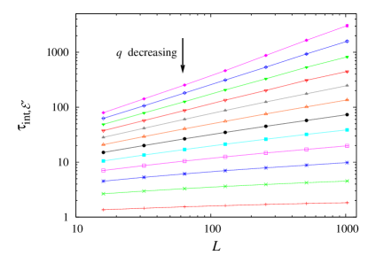
The autocorrelation functions of ${\cal N}$, ${\cal E}^{\prime}$ and ${\cal S}_{m}$ are in all cases very close to a pure exponential. In Fig. 1 we plot $\tau_{{\rm int},{\cal E}^{\prime}}$ (for $k=1$) versus $L$, and in Table 1 we report the estimated dynamic critical exponents $z_{{\rm int},{\cal E}^{\prime}}$. Our data also show that, as expected, the exponents are independent of $k$, and we have roughly $\tau\propto 1/k$.

Figure 2: Integrated autocorrelation times $\tau_{{\rm int},{\cal E}^{\prime}}$ divided by specific heat $C_{H}$, versus lattice size $L$, for the critical two-dimensional random-cluster model at $1.25\leq q\leq 4$, simulated using the Chayes–Machta algorithm with $k=1$.

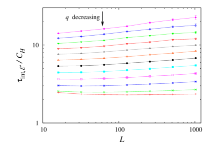
Since the Li–Sokal bound $\tau_{{\rm int},{\cal N}},\tau_{{\rm int},{\cal E}^{\prime}}\geq{\rm const}\times C_{H}$ and hence $z_{{\rm int},{\cal N}},z_{{\rm int},{\cal E}^{\prime}}\geq\alpha/\nu$, originally proven Li-Sokal for the Swendsen–Wang algorithm, can also be proven cm_3d for the Chayes–Machta algorithm (at least for ${\cal N}$), it is of interest to analyze its possible sharpness note_q=4 . In Fig. 2 we plot $\tau_{{\rm int},{\cal E}^{\prime}}/C_{H}$ versus $L$, in an attempt to determine whether this ratio is bounded or not as $L\to\infty$. The results are far from clear, but our best guess is that $\tau_{{\rm int},{\cal E}^{\prime}}/C_{H}$ diverges as $L\to\infty$, either as a small power or as a logarithm. However, the precise behavior needs to be explored by simulations at larger $L$.

On the other hand, Ossola and Sokal Ossola-Sokal recently conjectured, on the basis of the “data points” $(d,q)=(2,2)$, (2,3), (2,4), (3,2) and (4,2), that $z_{{\rm int},{\cal E}^{\prime}}\geq\beta/\nu$; and they even speculated that we might have the equality $z_{{\rm int},{\cal E}^{\prime}}=\max(\alpha/\nu,\beta/\nu)$. The data for noninteger $q$ now shed light on this conjecture: for $q=1.25,\,1.5$ there is modest evidence (and for $q=1.75$ there is weak evidence) that $z_{{\rm int},{\cal E}^{\prime}}<\beta/\nu$, i.e. that even the weak form of the Ossola–Sokal conjecture is false.

We next performed simulations on the simple-cubic lattice ($d=3$) for $q=1.5,\,1.8,\,2.2$ (see also Ossola-Sokal for $q=2$) and lattice sizes $4\leq L\leq 256$, using $k=$ the largest integer $\leq q$. We located the critical point by a finite-size-scaling analysis using the ratio $R=\langle{\cal S}_{4}\rangle/\langle{\cal S}_{2}^{2}\rangle$, as in forests_3d4d_prl . The complete set of runs used approximately 21.5 yr CPU time on a 3.2 GHz Xeon EM64T processor.

Figure 3: $k\,\tau_{{\rm int},{\cal E}^{\prime}}$ versus lattice size $L$ for Chayes–Machta simulations of the three-dimensional random-cluster model with $q=1.5,\,1.8,\,2.2$ at three near-critical temperatures, taking $k=\lfloor q\rfloor$. Data for $q=2$, $k=2$ at approximate criticality are from Ossola-Sokal .

$q$	Fit	$L_{\rm min}$	$z_{{\rm int},{\cal E}^{\prime}}$	$\alpha/\nu$	$\beta/\nu$
1.5	$AL^{z}$	96	0.13(1)	$-0.32(4)$	0.500(4)
1.8	$AL^{z}$	96	0.29(1)	$-0.15(5)$	0.5117(6)
2	$AL^{z}$	96	0.46(3)	0.174(1)	0.5184(1)
2.2	$AL^{z}$	24	0.76(1)	0.50(4)	0.508(4)

Table 2: Dynamic critical exponents $z_{{\rm int},{\cal E}^{\prime}}$ and static exponents $\alpha/\nu$ and $\beta/\nu$ for three-dimensional random-cluster model. For $q=2$, dynamic data are from Ossola-Sokal and static exponents are from d=3_Ising .

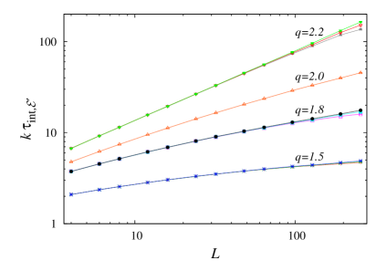
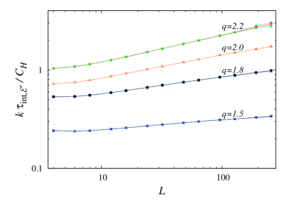
The autocorrelation functions of ${\cal N}$, ${\cal E}^{\prime}$ and ${\cal S}_{m}$ are again very close to a pure exponential. In Fig. 3 we plot $k\tau_{{\rm int},{\cal E}^{\prime}}$ versus $L$ (multiplying by $k$ makes the results for different $q$ comparable) for three temperatures very near criticality. In Table 2 we report the estimated dynamic critical exponents $z_{{\rm int},{\cal E}^{\prime}}$ and static critical exponents $\alpha/\nu$ and $\beta/\nu$. In Fig. 4 we plot $k\tau_{{\rm int},{\cal E}^{\prime}}/C_{H}$ versus $L$. It seems clear that, for all four values of $q$, the Li–Sokal bound is far from sharp. On the other hand, from Table 2 it seems clear that for $q=1.5,\,1.8$ we have the strict inequality $z_{{\rm int},{\cal E}^{\prime}}<\beta/\nu$, once again ruling out the Ossola–Sokal conjecture even in its weak form.

Figure 4: $k\,\tau_{{\rm int},{\cal E}^{\prime}}/C_{H}$ versus lattice size $L$ for Chayes–Machta simulations of the near-critical three-dimensional random-cluster model at $q=1.5,\,1.8,\,2,\,2.2$, with $k=\lfloor q\rfloor$. Data for $q=2$ at approximate criticality are from Ossola-Sokal .

The dynamic critical behavior of the SW–CM dynamic universality class in dimension $d=3$ therefore remains a mystery. Clearly, some new physical principle, beyond the slow equilibration of the energy embodied in the Li–Sokal bound Li-Sokal , needs to be discovered.

One clue might be provided by our analysis cm_3d of the CM algorithm on the complete graph (mean-field limit), generalizing the analysis in PeBeKaDo96 of the SW algorithm. Taking $k=1$ and defining a “magnetization” $m$ to be the fraction of sites in the largest cluster, we obtain for $1\leq q\leq 2$ the approximate difference equation (generalizing (PeBeKaDo96, , eq. (10)))

$$m^{\prime}\,=\,\frac{2q-2}{q}m-\frac{4t}{q^{2}}+\frac{8(q-1)tm}{3q^{2}}-\frac{2(q-1)^{2}m^{2}}{3q}\;$$ (5)

where $m^{\prime}$ is the value of $m$ after a sweep in which the active group contains the largest cluster, and $t$ is the deviation from the critical temperature. Clearly $q=2$ is a special case because the coefficient of the linear term equals 1: we have $\beta=1/2$ and $z=1$, and it is clear from the derivations PeBeKaDo96 ; cm_3d that $z$ is actually $\beta/\nu$. For $1\leq q<2$, by contrast, both the statics and dynamics are in the percolation universality class with $\beta=1$ and $z=0$: small perturbations from equilibrium relax exponentially with a finite autocorrelation time $\tau_{{\rm exp},m}=q/\log[q/(2q-2)]$ that diverges as $q\uparrow 2$. We conjecture that a similar behavior holds above the upper critical dimension, which for $q<2$ is presumably $d=6$. Our numerical data cm_3d confirm the behavior $z=0$ for $1\leq q<2$ with $\tau\propto 1/(2-q)$ as $q\uparrow 2$, but not the predicted amplitude.

Details of these simulations and their data analysis will be reported separately cm_2d ; cm_3d .