Sample eigenvalue based detection of high-dimensional signals in white noise using relatively few samples

Abstract

The detection and estimation of signals in noisy, limited data is a problem of interest to many scientific and engineering communities. We present a mathematically justifiable, computationally simple, sample eigenvalue based procedure for estimating the number of high-dimensional signals in white noise using relatively few samples. The main motivation for considering a sample eigenvalue based scheme is the computational simplicity and the robustness to eigenvector modelling errors which are can adversely impact the performance of estimators that exploit information in the sample eigenvectors.

There is, however, a price we pay by discarding the information in the sample eigenvectors; we highlight a fundamental asymptotic limit of sample eigenvalue based detection of weak/closely spaced high-dimensional signals from a limited sample size. This motivates our heuristic definition of the effective number of identifiable signals which is equal to the number of “signal” eigenvalues of the population covariance matrix which exceed the noise variance by a factor strictly greater than $1+\sqrt{\frac{\textrm{Dimensionality of the system}}{\textrm{Sample size}}}$.

The fundamental asymptotic limit brings into sharp focus why, when there are too few samples available so that the effective number of signals is less than the actual number of signals, underestimation of the model order is unavoidable (in an asymptotic sense) when using any sample eigenvalue based detection scheme, including the one proposed herein. The analysis reveals why adding more sensors can only exacerbate the situation. Numerical simulations are used to demonstrate that the proposed estimator, like Wax and Kailath’s MDL based estimator, consistently estimates the true number of signals in the dimension fixed, large sample size limit and the effective number of identifiable signals, unlike Wax and Kailath’s MDL based estimator, in the large dimension, (relatively) large sample size limit.

I Introduction

The observation vector, in many signal processing applications, can be modelled as a superposition of a finite number of signals embedded in additive noise. Detecting the number of signals present becomes a key issue and is often the starting point for the signal parameter estimation problem. When the signals and the noise are assumed, as we do in this paper, to be samples of a stationary, ergodic Gaussian vector process, the sample covariance matrix formed from $m$ observations has the Wishart distribution [1]. This paper uses an information theoretic approach, inspired by the seminal work of Wax and Kailath [2], for determining the number of signals in white noise from the eigenvalues of the Wishart distributed empirical covariance matrix formed from relatively few samples.

The reliance of the Wax and Kailath estimator and their successors [3, 4, 5, 6, 7], to list a few, on the distributional properties of the eigenvalues of non-singular Wishart matrices render them inapplicable in high-dimensional, sample starved settings where the empirical covariance matrix is singular. Ad-hoc modifications to such estimators are often not mathematically justified and it is seldom clear, even using simulations as in [5], whether a fundamental limit of detection is being encountered vis a vis the chronically reported symptom of underestimating the number of signals.

This paper addresses both of these issues using relevant results [8, 9, 10, 11] from large random matrix theory. The main contributions of this paper are 1) the development of a mathematically justified, computationally simple, sample eigenvalue based signal detection algorithm that operates effectively in sample starved settings and, 2) the introduction of the concept of effective number of (identifiable) signals which brings into sharp focus a fundamental limit in the identifiability, under sample size constraints, of closely spaced/low level signals using sample eigenvalue based detection techniques of the sort developed in this paper.

The proposed estimator exploits the distributional properties of the trace of powers, i.e., the moments of the eigenvalues, of (singular and non-singular) Wishart distributed large dimensional sample covariance matrices. The definition of effective number of identifiable signals is based on the mathematically rigorous results of Baik-Silverstein [12], Paul [13] and Baik et al [14] and the heuristic derivation of the first author [15]. This concept captures the fundamental limit of sample eigenvalue based detection by explaining why, in the large system relatively large sample size limit, if the signal level is below a threshold that depends on the noise variance, sample size and the dimensionality of the system, then reliable sample eigenvalue based detection is not possible. This brings into sharp focus the fundamental undetectability of weak/closely spaced signals using sample eigenvalue based schemes when too few samples are available. Adding more sensors will only exacerbate the problem by raising the detectability threshold.

Conversely, if the signal level is above this threshold, and the dimensionality of the system is large enough, then reliable detection using the proposed estimator is possible. We demonstrate this via numerical simulations that illustrate the superiority of the proposed estimator with the respect to the Wax-Kailath MDL based estimator. Specifically, simulations reveal that while both the new estimator and the Wax-Kailath MDL estimator are consistent estimators of the number of signals $k$ in the dimensionality $n$ fixed, sample size $m\to\infty$ sense, the MDL estimator is an inconsistent estimator of the effective number of signals in the large system, large sample size limit, i.e., in $n,m(n)\to\infty$ limit where the ratio $n/m(n)\to c\in(0,\infty)$ sense. Simulations suggest that the new estimator is a consistent estimator of the effective number of signals in the $n,m(n)\to\infty$ with $n/m(n)\to c\in(0,\infty)$ sense. We note that simulations will demonstrate the applicability of the proposed estimator in moderate dimensional settings as well.

The paper is organized as follows. The problem formulation in Section II is followed by a summary in Section III of the relevant properties of the eigenvalues of large dimensional Wishart distributed sample covariance matrices. An estimator for the number of signals present that exploits these results is derived in Section IV. An extension of these results to the frequency domain is discussed in Section V. Consistency of the proposed estimator and the concept of effective number of signals is discussed in Section VI. Simulation results that illustrate the superior performance of the new method in high dimensional, sample starved settings are presented in Section VII; some concluding remarks are presented in Section VIII.

II Problem formulation

We observe $m$ samples (“snapshots”) of possibly signal bearing $n$-dimensional snapshot vectors ${\bf x}_{1},\ldots,{\bf x}_{m}$ where for each $i$, ${\bf x}_{i}\sim\mathcal{N}_{n}(0,{\bf R})$ and ${\bf x}_{i}$ are mutually independent. The snapshot vectors are modelled as

$${\bf x}_{i}=\begin{cases}\,{\bf z}_{i}&\textrm{No Signal}\\ {\bf A}\,{\bf s}_{i}+{\bf z}_{i}&\textrm{Signal Present}\\ \end{cases}\qquad\textrm{for }i=1,\ldots,m,$$ (1)

where ${\bf z}_{i}\sim\mathcal{N}_{n}(0,\sigma^{2}{\bf I})$, denotes an $n$-dimensional (real or circularly symmetric complex) Gaussian noise vector where $\sigma^{2}$ is assumed to be unknown, ${\bf s}_{i}\sim\mathcal{N}_{k}({\bf 0},{\bf R}_{s})$ denotes a $k$-dimensional (real or circularly symmetric complex) Gaussian signal vector with covariance ${\bf R}_{s}$, and ${\bf A}$ is a $n\times k$ unknown non-random matrix. In array processing applications, the $j$-th column of the matrix ${\bf A}$ encodes the parameter vector associated with the $j$-th signal whose magnitude is described by the $j$-the element of ${\bf s}_{i}$.

Since the signal and noise vectors are independent of each other, the covariance matrix of ${\bf x}_{i}$ can be decomposed as

$${\bf R}={\bf\Psi}+\sigma^{2}{\bf I}$$ (2)

where

$${\bf\Psi}={\bf A}{\bf R}_{s}{\bf A}^{\prime},$$ (3)

with ^′ denoting the conjugate transpose. Assuming that the matrix ${\bf A}$ is of full column rank, i.e., the columns of ${\bf A}$ are linearly independent, and that the covariance matrix of the signals ${\bf R}_{s}$ is nonsingular, it follows that the rank of ${\bf\Psi}$ is $k$. Equivalently, the $n-k$ smallest eigenvalues of ${\bf\Psi}$ are equal to zero.

If we denote the eigenvalues of ${\bf R}$ by $\lambda_{1}\geq\lambda_{2}\geq\ldots\geq\lambda_{n}$ then it follows that the smallest $n-k$ eigenvalues of ${\bf R}$ are all equal to $\sigma^{2}$ so that

$$\lambda_{k+1}=\lambda_{k+2}=\ldots=\lambda_{n}=\lambda=\sigma^{2}.$$ (4)

Thus, if the true covariance matrix ${\bf R}$ were known apriori, the dimension of the signal vector $k$ can be determined from the multiplicity of the smallest eigenvalue of ${\bf R}$. When there is no signal present, all the eigenvalues of ${\bf R}$ will be identical. The problem in practice is that the covariance matrix ${\bf R}$ is unknown so that such a straight-forward algorithm cannot be used. The signal detection and estimation problem is hence posed in terms of an inference problem on $m$ samples of $n$-dimensional multivariate real or complex Gaussian snapshot vectors.

Inferring the number of signals from these $m$ samples reduces the signal detection problem to a model selection problem for which there are many approaches. A classical approach to this problem, developed by Bartlett [16] and Lawley [17], uses a sequence of hypothesis tests. Though this approach is sophisticated, the main problem is the subjective judgement needed by the practitioner in selecting the threshold levels for the different tests.

Information theoretic criteria for model selection such as those developed by Akaike [18, 19], Schwartz [20] and Rissanen [21] address this problem by proposing the selection of the model which gives the minimum information criteria. The criteria for the various approaches is generically a function of the log-likelihood of the maximum likelihood estimator of the parameters of the model and a term which depends on the number of parameters of the model that penalizes overfitting of the model order.

For the problem formulated above, Kailath and Wax [2] propose an estimator for the number of signals (assuming $m>n$ and ${\bf x}_{i}\in\mathbb{C}^{n}$) based on the eigenvalues $l_{1}\geq l_{2}\geq\ldots\geq l_{n}$ of the sample covariance matrix (SCM) defined by

$$\widehat{{\bf R}}=\frac{1}{m}\sum_{i=1}^{m}{\bf x}_{i}{\bf x}_{i}^{\prime}=\frac{1}{m}{\bf X}{\bf X}^{\prime}$$ (5)

where ${\bf X}=[{\bf x}_{1}|\ldots|{\bf x}_{m}]$ is the matrix of observations (samples). The Akaike Information Criteria (AIC) form of the estimator is given by

$$\hat{k}_{{\rm AIC}}=\operatornamewithlimits{\arg\min}-2(n-k)m\log\frac{g(k)}{a(k)}+2k(2n-k)\qquad\textrm{for }k\in\mathbb{N}:0\leq k<n$$ (6)

while the Minimum Descriptive Length (MDL) criterion is given by

$$\hat{k}_{{\rm MDL}}=\operatornamewithlimits{\arg\min}-(n-k)m\log\frac{g(k)}{a(k)}+\frac{1}{2}k(2n-k)\log m\qquad\textrm{for }k\in\mathbb{N}:0\leq k<n$$ (7)

where $g(k)=\prod_{j=k+1}^{n}l_{j}^{1/(n-k)}$ is the geometric mean of the $n-k$ smallest sample eigenvalues and $a(k)=\frac{1}{n-k}\sum_{j=k+1}^{n}l_{j}$ is their arithmetic mean.

It is known [2] that the AIC form inconsistently estimates the number of signals, while the MDL form estimates the number of signals consistently in the classical $n$ fixed, $m\to\infty$ sense. The simplicity of the estimator, and the large sample consistency are among the primary reasons why the Kailath-Wax MDL estimator continues to be employed in practice [22]. In the two decades since the publication of the WK paper, researchers have come up with many innovative solutions for making the estimators more “robust” in the sense that estimators continue to work well in settings where the underlying assumptions of snapshot and noise Gaussianity and inter-snapshot independence (e.g. in the presence of multipath) can be relaxed as in the work of Zhao et al [23, 24], Xu et al [3], and Stoica-Cedervall [25]among others [26].

Despite its obvious practical importance, the robustness of the algorithm to model mismatch is an issue that we shall not address in this paper. Instead we aim to revisit the original problem considered by Wax and Kailath with the objective of designing an estimator that is robust to high-dimensionality and sample size constraints. We are motivated by the observation that the most important deficiency of the Wax-Kailath estimator and its successors that is yet to be satisfactorily resolved occurs in the setting where the sample size is smaller than the number of sensors, i.e., when $m<n$, which is increasingly the case in many state-of-the-art radar and sonar systems where the number of sensors exceeds the sample size by a factor of $10-100$ [27]. In this situation, the SCM is singular and the estimators become degenerate, as seen in (6) and (7). Practitioners often overcome this in an ad-hoc fashion by, for example, restricting $k$ in (7) to integer values in the range $0\leq k<\min(n,m)$ so that

$$\hat{k}_{\overline{{\rm MDL}}}=\operatornamewithlimits{\arg\min}-(n-k)m\log\frac{g(k)}{a(k)}+\frac{1}{2}k(2n-k)\log m\qquad\textrm{for }k\in\mathbb{N}:0\leq k<\min(n,m)$$ (8)

Since large sample, i.e., $m\gg n$, asymptotics [28] were used to derive the estimators in [2], there is no rigorous theoretical justification for such a reformulation even if the simulation results suggest that the WK estimators are working “well enough.”

This is true for other sample eigenvalue based solutions found in the literature that exploit the sample eigenvalue order statistics [6, 7], employ a Bayesian framework by imposing priors on the number of signals [29], involve solving a set of possibly high-dimensional non-linear equations [3], or propose sequential hypothesis testing procedures [4]. The fact that these solutions are computationally more intensive or require the practitioner to set subjective threshold levels makes them less attractive than the WK MDL solution; more importantly, they do not address the sample starved setting in their analysis or their simulations either.

For example, in [7], Fishler et al use simulations to illustrate the performance of their algorithm with $n=7$ sensors and a sample size $m>500$ whereas in a recent paper [26], Fishler and Poor illustrate their performance with $n=10$ sensors and $m>50$ samples. Van Trees discusses the various techniques for estimating the number of signals in Section 7.8 of [22]; the sample starved setting where $m=O(n)$ or $m<n$ is not treated in the simulations either.

There is however, some notable work on detecting the number of signals using short data records. Particle filter based techniques [30], have proven to be particularly useful in such short data record settings. Their disadvantage, from our perspective, is that they require the practitioner to the model the eigenvectors of the underlying population covariance matrix as well; this makes them especially sensitive to model mismatch errors that are endemic to high-dimensional settings.

This motivates our development of a mathematically justifiable, sample eigenvalue based estimator with a computational complexity comparable to that of the modified WK estimator in (8) that remains robust to high-dimensionality and sample size constraints. The proposed new estimator given by:

$\displaystyle t_{k}$ $\displaystyle=\left[(n-k)\dfrac{\sum_{i=k+1}^{n}l_{i}^{2}}{(\sum_{i=k+1}^{n}l_{i})^{2}}-\left(1+\dfrac{n}{m}\right)\right]n-\left(\dfrac{2}{\beta}-1\right)\dfrac{n}{m}$ (9a) $\displaystyle\hat{k}_{{\rm NEW}}$ $\displaystyle=\operatornamewithlimits{\arg\min}_{k}\,\left\{\dfrac{\beta}{4}\left[\dfrac{m}{n}\right]^{2}\,t_{k}^{2}\right\}+2(k+1)\qquad\textrm{for }k\in\mathbb{N}:0\leq k<\min(n,m).\$ (9b) Here $\beta=1$ if ${\bf x}_{i}\in\mathbb{R}^{n}$, and $\beta=2$ if ${\bf x}_{i}\in\mathbb{C}^{n}$. In (9), the $l_{i}$’s are the eigenvalues of the sample covariance matrix $\widehat{{\bf R}}$. An implicit assumption in the derivation of (9) is that the number of signals is much smaller than the system size, i.e., $k\ll n$. A rather important consequence of our sample eigenvalue based detection scheme, as we shall elaborate in Section VI, is that it just might not be possible to detect low level/closely spaced signals when there are too few samples available.

To illustrate this effect, consider the situation where there are two uncorrelated (hence, independent) signals so that ${\bf R}_{s}=\textrm{diag}(\sigma_{{\rm S}1}^{2},\sigma_{{\rm S}2}^{2})$. In (1) let ${\bf A}=[{\bf v}_{1}{\bf v}_{2}]$, as in a sensor array processing application so that ${\bf v}_{1}\equiv{\bf v}(\theta_{1})$ and ${\bf v}_{2}\equiv{\bf v}_{2}(\theta_{2})$ encode the array manifold vectors for a source and an interferer with powers $\sigma_{{\rm S}1}^{2}$ and $\sigma_{{\rm S}2}^{2}$, located at $\theta_{1}$ and $\theta_{2}$, respectively. The covariance matrix is then given by

$${\bf R}=\sigma_{{\rm S}1}^{2}{\bf v}_{1}{\bf v}_{1}^{\prime}+\sigma_{{\rm S}2}^{2}{\bf v}_{2}{\bf v}_{2}^{\prime}+\sigma^{2}{\bf I}.$$ (10)

In the special situation when $\parallel\!{\bf v}_{1}\!\parallel=\parallel\!{\bf v}_{2}\!\parallel=\parallel\!{\bf v}\!\parallel$ and $\sigma_{{\rm S1}}^{2}=\sigma_{{\rm S2}}^{2}=\sigma_{{\rm S}}^{2}$, we can (in an asymptotic sense) reliably detect the presence of both signals from the sample eigenvalues alone whenever

$$\textrm{Asymptotic identifiability condition}:\qquad\sigma_{{\rm S}}^{2}\parallel\!{\bf v}\!\parallel^{2}\left(1-\dfrac{|\langle{\bf v}_{1},{\bf v}_{2}\rangle|}{\parallel\!{\bf v}\parallel}\right)>\sigma^{2}\sqrt{\dfrac{n}{m}}$$ (11)

If the signals are not strong enough or not spaced far enough part, then not only will proposed estimator consistently underestimate the number of signals but so will any other sample eigenvalue based detector.

The concept of the effective number of signals provides insight into the fundamental limit, due to snapshot constraints in high-dimensional settings, of reliable signal detection by eigen-inference , i.e., by using the sample eigenvalues alone. This helps identify scenarios where algorithms that exploit any structure in the eigenvectors of the signals, such as the MUSIC and the Capon-MVDR algorithms in sensor array processing [22] or particle filter based techniques [30], might be better able to tease out lower level signals from the background noise. It is worth noting that the proposed approach remain relevant in situations where the eigenvector structure has been identified. This is because eigen-inference methodologies are inherently robust to eigenvector modelling errors that occur in high-dimensional settings. Thus the practitioner may use the proposed methodologies to complement and “robustify” the inference provided by algorithms that exploit the eigenvector structure.

III Pertinent results from random matrix theory

Analytically characterizing the distribution of the sample eigenvalues, as a function of the population eigenvalues, is the first step in designing a sample eigenvalue based estimator that is robust to high-dimensionality and sample size constraints. For arbitrary covariance ${\bf R}$, the joint density function of the eigenvalues $l_{1},\ldots,l_{n}$ of the SCM $\widehat{\bf R}$ when $m>n+1$ is shown to be given by [28]

$$f(l_{1},\ldots,l_{n})=\widetilde{Z}_{n,m}^{\beta}\sum_{i=1}^{n}l_{i}^{\beta(m-n+1)/2-1}\prod_{i<j}^{n}|l_{i}-l_{j}|^{\beta}\prod_{i=1}^{n}dl_{i}\int_{{\bf Q}}\exp\left(-\dfrac{m\beta}{2}\,\mathrm{Tr}\,\left({\bf R}^{-1}{\bf Q}\widehat{\bf R}{\bf Q}^{\prime}\right)\right)d{\bf Q}$$ (12)

where $l_{1}>\ldots>l_{n}>0$, $\widetilde{Z}_{n,m}^{\beta}$ is a normalization constant, and $\beta=1$ (or $2$) when $\widehat{\bf R}$ is real (resp. complex). In (12), ${\bf Q}\in{\bf O}(n)$ when $\beta=1$ while ${\bf Q}\in{\bf U}(n)$ when $\beta=2$ where ${\bf O}(n)$ and ${\bf U}(n)$ are, respectively, the set of $n\times n$ orthogonal and unitary matrices with Haar measure.

Note that the exact characterization of the joint density of the eigenvalues in (12) involves a multidimensional integral over the orthogonal (or unitary) group. This makes it intractable for analysis without resorting to asymptotics. Anderson’s landmark paper [28] does just that by characterizing the distribution of the sample eigenvalues using large sample asymptotics. A classical result due to Anderson establishes the consistency of the sample eigenvalues in the dimensionality $n$ fixed, sample size $m\to\infty$ asymptotic regime [28]. When the dimensionality is small and there are plenty of samples available, Anderson’s analysis suggests that the sample eigenvalues will be (roughly) symmetrically centered around the population eigenvalues. When the dimensionality is large, and the sample size is relatively small, Anderson’s prediction of sample eigenvalue consistency is in stark contrast to the asymmetric spreading of the sample eigenvalues that is observed in numerical simulations. This is illustrated in Figure 1 where the $n=20$ eigenvalues of a SCM formed from $m=20$ samples are compared with the eigenvalues of the underlying population covariance matrix.

(a) True Eigenvalues.

(b) Sample eigenvalues formed from $20$ snapshots.

Figure 1: Blurring of sample eigenvalues relative to the population eigenvalues when are there a finite number of snapshots.

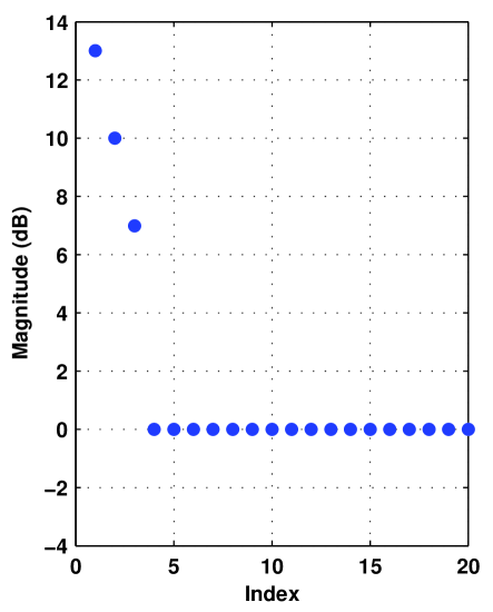
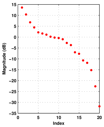
The role of random matrix theory comes in because of new analytical results that are able to precisely describe the spreading of the sample eigenvalues exhibited in Figure 1. Since our new estimator explicitly exploits these analytical results, the use of our estimator in high-dimensional, sample starved settings is more mathematically justified than other sample eigenvalue based approaches found in the literature that explicitly use Anderson’s sample eigenvalue consistency results. See, for example [2, Eq. (13a), pp. 389], [6, Eq (5)., pp. 2243].

We argue that this is particularly so in settings where $m<n$, where practitioners (though, not the original authors!) have often invoked the equality between the non-zero eigenvalues of the $\widehat{{\bf R}}=(1/m){\bf X}{\bf X}^{\prime}$ and the matrix $(1/m){\bf X}^{\prime}{\bf X}$ to justify ad-hoc modifications to estimators that use only the non-zero eigenvalues of the SCM, as in (8). We contend that such an ad-hoc modification to any estimator that explicitly uses Anderson’s sample eigenvalue consistency results is mathematically unjustified because the sample eigen-spectrum blurring, which is only exacerbated in the $m<n$ regime, remains unaccounted for.

Before summarizing the pertinent results, we note that the analytical breakthrough is a consequence of considering the large system size, relatively large sample size asymptotic regime as opposed to “classical” fixed system size, large sample size asymptotic regime. Mathematically speaking, the new results describe the distribution of the eigenvalues in $n,m\to\infty$ with $n/m\to c\in(0,\infty)$ asymptotic regime as opposed to the $n$ fixed, $m\to\infty$ regime à la Anderson. We direct the reader to Johnstone’s excellent survey for a discussion on these asymptotic regimes [31, pp. 9] and much more.

III-A Eigenvalues of the signal-free SCM

A central object in the study of large random matrices is the empirical distribution function (e.d.f.) of the eigenvalues, which for an arbitrary matrix ${\bf A}$ with $n$ real eigenvalues (counted with multiplicity), is defined as

$$F^{{\bf A}}(x)=\frac{\textrm{Number of eigenvalues of }{\bf A}\leq x}{n}.$$ (13)

For a broad class of random matrices, the sequence of e.d.f.’s can be shown to converge in the $n\to\infty$ limit to a non-random distribution function [32]. Of particular interest is the convergence of the e.d.f. of the signal-free SCM which is described next.

Proposition III.1

Let $\widehat{{\bf R}}$ denote a signal-free sample covariance matrix formed from an $n\times m$ matrix of observations with i.i.d. Gaussian samples of mean zero and variance $\lambda=\sigma^{2}$. Then the e.d.f. $F^{{\widehat{\bf R}}}(x)\to F^{W}(x)$ almost surely for every $x$, as $m,n\to\infty$ and $c_{m}=n/m\to c$ where

$$dF^{W}(x)=\max\left(0,\left(1-\frac{1}{c}\right)\right)\delta(x)+\frac{\sqrt{(x-a_{-})(a_{+}-x)}}{2\pi\lambda xc}\mathbb{I}_{[a_{-},a_{+}]}(x)\,dx,$$ (14)

with $a_{\pm}=\lambda(1\pm\sqrt{c})^{2}$, $\mathbb{I}_{[a,b]}(x)=1$ when $a\leq x\leq b$ and zero otherwise, and $\delta(x)$ is the Dirac delta function.

Proof:

This result was proved in [33, 34] in very general settings. Other proofs include [9, 35, 36]. The probability density in (14) is often referred to as the Marčenko-Pastur density. ∎

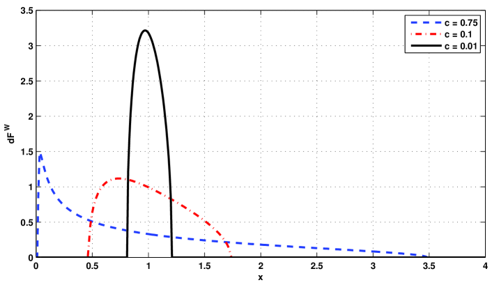
Figure 2 plots the Marčenko-Pastur density in (14) for $\lambda=1$ and different values of $c=\lim n/m$. Note that as $c\to 0$, the eigenvalues are increasingly clustered around $x=1$ but for modest values of $c$, the spreading is quite significant.

Figure 2: The Marčenko-Pastur density, given (14), for the eigenvalues of the signal-free sample covariance matrix with noise variance $1$ and $c=\lim n/m$.

The almost sure convergence of the e.d.f. of the signal-free SCM implies that the moments of the eigenvalues converge almost surely, so that

$$\frac{1}{n}\sum_{i=1}^{n}l_{i}^{k}\overset{a.s.}{\longrightarrow}\int x^{k}dF^{W}(x)=:M^{W}_{k}.$$ (15)

The moments of the Marčenko-Pastur density are given by [9, 37]

$$M^{W}_{k}=\lambda^{k}\sum_{j=0}^{k-1}c^{j}\frac{1}{j+1}{k\choose j}{k-1\choose j}.$$ (16)

For finite $n$ and $m$, the sample moments, i.e., $\frac{1}{n}\sum_{i=1}^{n}l_{i}^{k}$ will fluctuate about these limiting values. The precise nature of the fluctuations is described next.

Proposition III.2

If $\widehat{{\bf R}}$ satisfies the hypotheses of Proposition III.1 for some $\lambda$ then as $m,n\to\infty$ and $c_{m}=n/m\to c\in(0,\infty)$, then

$$n\,\left(\begin{bmatrix}\frac{1}{n}\sum_{i=1}^{n}l_{i}\\ \\ \frac{1}{n}\sum_{i=1}^{n}l_{i}^{2}\end{bmatrix}-\begin{bmatrix}\lambda\\ \\ \lambda^{2}(1+c)\end{bmatrix}\right)\overset{\mathcal{D}}{\longrightarrow}\mathcal{N}\left(\underbrace{\begin{bmatrix}0\\ (\frac{2}{\beta}-1)\lambda^{2}c\end{bmatrix}}_{={\bm{\mu}_{Q}}},\frac{2}{\beta}\underbrace{\begin{bmatrix}\lambda^{2}c&2\lambda^{3}c\,(c+1)\\ 2\lambda^{3}c\,(c+1)&2\lambda^{4}c\,(2c^{2}+5c+2)\\ \end{bmatrix}}_{={\bf Q}}\right)$$ (17)

where the convergence is in distribution.

Proof:

This result appears in [8, 9] for the real case and in [10] for the real and complex cases. The result for general $\beta$ appears in Dumitriu and Edelman [11]. ∎

We now use the result in Proposition III.2 to develop a test statistic $q_{n}$ whose distribution is independent of the unknown noise variance $\lambda$. The distributional properties of this test statistic are described next.

Proposition III.3

Assume $\widehat{{\bf R}}$ satisfies the hypotheses of Proposition III.1 for some $\lambda$. Consider the statistic

$$q_{n}=\dfrac{\frac{1}{n}\sum_{i=1}^{n}l_{i}^{2}}{\left(\frac{1}{n}\sum_{i=1}^{n}l_{i}\right)^{2}}.$$

Then as $m,n\to\infty$ and $c_{m}=n/m\to c\in(0,\infty)$,

$$n\left[q_{n}-(1+c)\right]\overset{\mathcal{D}}{\longrightarrow}\mathcal{N}\left(\left(\dfrac{2}{\beta}-1\right)c,\dfrac{4}{\beta}c^{2}\right)$$ (18)

where the convergence is in distribution.

Proof:

Define the function $g(x,y)=y/x^{2}$. Its gradient vector $\bm{\nabla}\!g(x,y)$ is given by

$$\bm{\nabla}\!g(x,y):=[\partial_{x}g(x,y)\,\,\,\>\>~{}~{}\partial_{y}g(x,y)]^{T}=[-2y/x^{3}\,\,\,\>\>~{}~{}~{}1/x^{2}]^{T}.$$ (19)

The statistic $q_{n}$ can be written in terms of $g(x,y)$ as simply $q_{n}=g(\frac{1}{n}\sum_{i=1}^{n}l_{i},\frac{1}{n}\sum_{i=1}^{n}l_{i}^{2})$. The limiting distribution of $q_{n}$ can be deduced from the distributional properties of $\frac{1}{n}\sum_{i=1}^{n}l_{i}$ and $\frac{1}{n}\sum_{i=1}^{n}l_{i}^{2}$ established in Proposition III.2. Specifically, by an application of the delta method [38], we obtain that as $n,m\to\infty$ with $n/m\to c\in(0,\infty)$,

$$n\left[q_{n}-g(\lambda,\lambda^{2}(1+c))\right]\overset{\mathcal{D}}{\longrightarrow}\mathcal{N}(\mu_{q},\sigma^{2}_{q})$$

where the mean $\mu_{q}$ and the variance $\sigma^{2}_{q}$ are given by

$$\mu_{q} =\bm{\mu}_{Q}^{T}\bm{\nabla}\!g\left(\lambda,\lambda^{2}(1+c)\right),$$ (20a)

$$\sigma^{2}_{q} =\dfrac{2}{\beta}\bm{\nabla}\!g\left(\lambda,\lambda^{2}(1+c)\right)^{T}{\bf Q}\bm{\nabla}\!g\left(\lambda,\lambda^{2}(1+c)\right)$$ (20b)

Substituting, the expressions for $\bm{\mu}_{Q}$ and ${\bf Q}$ given in (17), in (20a) and (20b) gives us the required expressions for the mean and the variance of the normal distribution on the right hand side of (18) ∎

III-B Eigenvalues of the signal bearing SCM

When there are $k$ signals present then, in the $n\to\infty$ limit, where $k$ is kept fixed, the limiting e.d.f. of $\widehat{{\bf R}}$ will still be given by Proposition III.1. This is because the e.d.f., defined as in (13), weights the contribution of every eigenvalue equally so that effect of the $k/n$ fraction of “signal” eigenvalues vanishes in the $n\to\infty$ limit.

Note, however, that in the signal-free case, i.e., when $k=0$, Proposition III.1 and the result in [39] establish the almost sure convergence of the largest eigenvalue of the SCM to $\lambda(1+\sqrt{c})^{2}$. In the signal bearing case, a so-called phase transition phenomenon is observed, in that the largest eigenvalue will converge to a limit different from that in the signal-free case only if the “signal” eigenvalues are above a certain threshold. This is described next.

Proposition III.4

Let $\widehat{{\bf R}}$ denote a sample covariance matrix formed from an $n\times m$ matrix of Gaussian observations whose columns are independent of each other and identically distributed with mean ${\bf 0}$ and covariance ${\bf R}$. Denote the eigenvalues of ${\bf R}$ by $\lambda_{1}\geq\lambda_{2}>\ldots\geq\lambda_{k}>\lambda_{k+1}=\ldots\lambda_{n}=\lambda$. Let $l_{j}$ denote the $j$-th largest eigenvalue of $\widehat{{\bf R}}$. Then as $n,m\to\infty$ with $c_{m}=n/m\to c\in(0,\infty)$,

$$l_{j}\to\begin{cases}\lambda_{j}\left(1+\dfrac{\lambda\,c}{\lambda_{j}-\lambda}\right)&{\rm if}\qquad\lambda_{j}>\lambda\,(1+\sqrt{c})\\ &\\ \lambda\,(1+\sqrt{c})^{2}&{\rm if}\qquad\lambda_{j}\leq\lambda(1+\sqrt{c})\\ \end{cases}$$ (21)

for $j=1,\ldots,k$ and the convergence is almost surely.

Proof:

This result appears in [12] for very general settings. A matrix theoretic proof for the real valued SCM case may be found in [13] while a determinental proof for the complex case may be found in [14]. A heuristic derivation that relies on an interacting particle system interpretation of the sample eigenvalues appears in [15]. ∎

For “signal” eigenvalues above the threshold described in Proposition III.4, the fluctuations about the asymptotic limit are described next.

Proposition III.5

Assume that $\widehat{{\bf R}}$ and ${\bf R}$ satisfy the hypotheses of Proposition III.4. If $\lambda_{j}>\lambda(1+\sqrt{c})$ has multiplicity $1$ and if $\sqrt{m}|c-n/m|\to 0$ then

$$\sqrt{n}\left[l_{j}-\lambda_{j}\left(1+\dfrac{\lambda\,c}{\lambda_{j}-\lambda}\right)\right]\overset{\mathcal{D}}{\longrightarrow}\mathcal{N}\left(0,\dfrac{2}{\beta}\lambda_{j}^{2}\left(1-\dfrac{c}{(\lambda_{j}-\lambda)^{2}}\right)\right)$$ (22)

where the convergence in distribution is almost surely.

Proof:

A matrix theoretic proof for the real case may be found in [13] while a determinental proof for the complex case may be found in [14]. The result has been strengthened for non-Gaussian situations by Baik and Silverstein for general $c\in(0,\infty)$ [40]. ∎

IV Estimating the number of signals

We derive an information theoretic estimator for the number of signals by exploiting the distributional properties of the moments of eigenvalues of the (signal-free) SCM given by Propositions III.2 and III.3, as follows. The overarching principle used is that, given an observation ${\bf y}=[y(1),\ldots,y(N)]$ and a family of models, or equivalently a parameterized family of probability densities $f({\bf y}|\bm{\theta})$ indexed by the parameter vector $\bm{\theta}$, we select the model which gives the minimum Akaike Information Criterion (AIC) [19] defined by

$${\rm AIC}_{k}=-2\log f({\bf y}|\widehat{\bm{\theta}})+2k$$ (23)

where $\widehat{\bm{\theta}}$ is the maximum likelihood estimate of $\bm{\theta}$, and $k$ is the number of free parameters in $\bm{\theta}$. Since the noise variance is unknown, the parameter vector of the model, denoted by $\bm{\theta}_{k}$, is given by

$$\bm{\theta}_{k}=[\lambda_{1},\ldots,\lambda_{k},\sigma^{2}]^{T}.$$ (24)

There are thus $k+1$ free parameters in $\bm{\theta}_{k}$. Assuming that there are $k<\min(n,m)$ signals, the maximum likelihood estimate of the noise variance is given by [28] (which Proposition III.2 corroborates in the $m<n$ setting)

$$\widehat{\sigma}^{2}_{(k)}=\dfrac{1}{n-k}\sum_{i=k+1}^{n}l_{i}$$ (25)

where $l_{1}\geq\ldots\geq l_{n}$ are the eigenvalues of $\widehat{{\bf R}}$. Consider the test statistic

$$q_{k} =n\left[\dfrac{\frac{1}{n-k}\sum_{i=k+1}^{n}l_{i}^{2}}{\left(\widehat{\sigma}^{2}_{(k)}\right)^{2}}-(1+c)\right]-\left(\dfrac{2}{\beta}-1\right)c$$ (26)

$$=n\left[\dfrac{\frac{1}{n-k}\sum_{i=k+1}^{n}l_{i}^{2}}{\left(\frac{1}{n-k}\sum_{i=k+1}^{n}l_{i}\right)^{2}}-(1+c)\right]-\left(\dfrac{2}{\beta}-1\right)c.$$ (27)

for a constant $c>0$. When $k>0$ signals are present and assuming $k\ll n$, then the distributional properties of the $n-k$ “noise” eigenvalues are closely approximated by the distributional properties of the eigenvalues given by Proposition III.2 of the signal-free SCM, i.e., when $k=0$. It is hence reasonable to approximate the distribution of the statistic $q_{k}$ with the normal distribution whose mean and variance, for some $c>0$, given in Proposition III.3. The log-likelihood function $\log f(q_{k}|\widehat{{\bf\theta}})$, for large $n,m$ can hence be approximated by

$$-\log f(q_{k}|\widehat{{\bf\theta}})\approx\dfrac{q_{k}^{2}}{2\frac{4}{\beta}c^{2}}+\underbrace{\dfrac{1}{2}\log 2\pi\frac{4}{\beta}c^{2}}_{{\rm Constant}}.$$ (28)

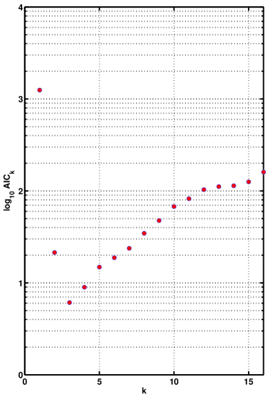
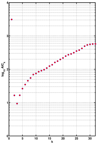
In (26), and (28), it is reasonable (Bai and Silverstein provide an argument in [10]) to use $c_{m}=n/m$ for the (unknown) limiting parameter $c=\lim n/m$. Plugging in $c\approx c_{m}=n/m$ into (26), and (28), ignoring the constant term on the right hand side of (28) when the log-likelihood function is substituted into (23) yields the estimator in (9). Figure 3 plots sample realizations of the score function.

(a) Complex signals: $n=16$, $m=32$.

(b) Complex signals: $n=32$, $m=64$.

Figure 3: Sample realizations of the proposed criterion when there $k=2$ complex valued signals and $\lambda_{1}=10$, $\lambda_{2}=3$ and $\lambda_{3}=\ldots=\lambda_{n}=1$.

V Extension to frequency domain and vector sensors

When the $m$ snapshot vectors ${\bf x}_{i}(w_{j})$ for $j=1,\ldots,m$ represent Fourier coefficients vectors at frequency $w_{j}$ then the sample covariance matrix

$$\widehat{{\bf R}}(w_{j})=\dfrac{1}{m}\sum_{i=1}^{m}{\bf x}_{i}(w_{j}){\bf x}_{i}(w_{j})^{\prime}$$ (29)

is the periodogram estimate of the spectral density matrix at frequency $w_{j}$. The time-domain approach carries over to the frequency domain so that the estimator in (9) remains applicable with $l_{i}\equiv l_{i}(w_{j})$ where $l_{1}(w_{j})\geq l_{2}(w_{j})\geq\ldots\geq l_{n}(w_{j})$ are the eigenvalues of $\widehat{{\bf R}}(w_{j})$.

When the signals are wideband and occupy $M$ frequency bins, denoted by $w_{1},\ldots,w_{M}$, then the information on the number of signals present is contained in all the bins. The assumption that the observation time is much larger than the correlation times of the signals (sometimes referred to as the SPLOT assumption - stationary process, long observation time) ensures that the Fourier coefficients corresponding to the different frequencies are statistically independent.

Thus the AIC based criterion for detecting the number of wideband signals that occupy the frequency bands $w_{1},\ldots,w_{M}$ is obtained by summing the corresponding criterion in (9) over the frequency range of interest:

$$t_{j,k}=\left[(n-k)\dfrac{\sum_{i=k+1}^{n}l_{i}(w_{j})^{2}}{(\sum_{i=k+1}^{n}l_{i}(w_{j}))^{2}}-\left(1+\dfrac{n}{m}\right)\right]n-\left(\dfrac{2}{\beta}-1\right)\dfrac{n}{m}$$ (30a) $$\hat{k}_{{\rm NEW}}=\operatornamewithlimits{\arg\min}_{k\in\mathbb{N}:0\leq k<\min(n,m)}\sum_{j=1}^{M}\dfrac{\beta}{4}\left[\dfrac{m}{n}\right]^{2}\,t_{j,k}^{2}+2M(k+1)$$ (30b)

When the number of snapshots is severely constrained, the SPLOT assumption is likely to be violated so that the Fourier coefficients corresponding to different frequencies will not be statistically independent. This will likely degrade the performance of the proposed estimators.

When the measurement vectors represent quaternion valued narrowband signals, then $\beta=4$ so that the estimator in (9) can be used. Quaternion valued vectors arise when the data collected from vector sensors is represented using quaternions as in [41].

VI Consistency of the estimator and the effective number of identifiable signals

For a fixed sample size, and system dimensionality, the probability of detecting a signal is the most practically useful criterion for comparing the performance of different estimators. For theoretical purposes, however, the large sample consistency of the estimator is (usually) more analytically tractable and hence often supplied as the justification for employing an estimator. We conjecture that the proposed algorithm is a consistent estimator of the true number of signals in the “classical” large sample asymptotic regime in the sense made explicit next.

Conjecture VI.1

Let ${\bf R}$ be a $n\times n$ covariance matrix that satisfies the hypothesis of Proposition III.4. Let $\widehat{{\bf R}}$ be a sample covariance matrix formed from $m$ snapshots. Then in the $n$ fixed, $m\to\infty$ limit, $\widehat{k}$ is a consistent estimator of $k$ where $\widehat{k}$ is the estimate of the number of signals obtained using (9).

The “classical” notion of large sample consistency does not adequately capture the suitability of an estimator in high dimensional, sample starved settings when $m<n$ or $m=O(n)$. In such settings, it is more natural to investigate the consistency properties of the estimator in the large system, large sample limit instead. We can use Proposition III.4 to establish an important property of the proposed estimator in such a limit.

Theorem VI.2

Let ${\bf R}$ and $\widetilde{{\bf R}}$ be two $n\times n$ sized covariance matrices whose eigenvalues are related as

$${\bf\Lambda}=\textrm{diag}(\lambda_{1},\ldots,\lambda_{p},\lambda_{p+1},\ldots,\lambda_{k},\lambda,\ldots,\lambda)$$ (31a)

$$\widetilde{{\bf\Lambda}}=\textrm{diag}(\lambda_{1},\ldots,\lambda_{p},\lambda,\ldots,\lambda)$$ (31b)

where for some $c\in(0,\infty)$, and all $i=p+1,\ldots,k$, $\lambda<\lambda_{i}\leq\lambda\,(1+\sqrt{c})$. Let $\widehat{{\bf R}}$ and $\widehat{\widetilde{{\bf R}}}$ be the associated sample covariance matrices formed from $m$ snapshots. Then for every $n,m(n)\to\infty$ such that $c_{m}=n/m\to c$,

$$\textrm{Prob}(\widehat{k}=j\,|\,{\bf R})\to\textrm{Prob}(\widehat{k}=j\,|\,\widetilde{{\bf R}})\qquad\textrm{for }j=1,\ldots,p$$ (32a)

and

$$\textrm{Prob}(\widehat{k}>p\,|\,{\bf R})\to\textrm{Prob}(\widehat{k}>p\,|\,\widetilde{{\bf R}})$$ (32b)

where the convergence is almost surely and $\widehat{k}$ is the estimate of the number of signals obtained using the algorithm in (9).

Proof:

The result follows from Proposition III.4. The almost sure convergence of the sample eigenvalues $l_{j}\to\lambda(1+\sqrt{c})^{2}$ for $j=p+1,\ldots,k$ implies that $i$-th largest eigenvalues of $\widehat{{\bf R}}$ and $\widehat{\widetilde{{\bf R}}}$, for $i=1,\ldots,p+1$, converge to the same limit almost surely. The fluctuations about this limit will hence be identical so that (32) follows in the asymptotic limit. ∎

Note that the rate of convergence to the asymptotic limit for $\textrm{Prob}(\widehat{k}>p\,|\,{\bf R})$ and $\textrm{Prob}(\widehat{k}>p\,|\,\widetilde{{\bf R}})$ will, in general, depend on the eigenvalue structure of ${\bf R}$ and may be arbitrarily slow. Thus, Theorem VI.2 yields no insight into rate of convergence type issues which are important in practice. Rather, the theorem is a statement on the asymptotic equivalence, from an identifiability point of view, of sequences of sample covariance matrices which are related in the manner described. At this point, we are unable to prove the consistency of the proposed estimator as this would require more a refined analysis that characterizes the fluctuations of subsets of the (ordered) “noise” eigenvalues. The statement regarding consistency of the proposed estimator, in the sense of large system, large sample limit, is presented as a conjecture with numerical simulations used as non-definitive yet corroborating evidence.

Conjecture VI.3

Let ${\bf R}$ be a $n\times n$ covariance matrix that satisfies the hypothesis of Proposition III.4. Let $\widehat{{\bf R}}$ be a sample covariance matrix formed from $m$ snapshots. Define $$k_{{\rm eff}}(c\,|\,{\bf R}):=\textrm{Number of eigenvalues of }{\bf R}>\lambda(1+\sqrt{c}).$$ (33) Then in $m,n\to\infty$ limit with $c_{m}=n/m\to c$, $\widehat{k}$ is a consistent estimator of $k_{{\rm eff}}(c)$ where $\widehat{k}$ is the estimate of the number of signals obtained using the algorithm in (9).
Motivated by Proposition III.4, we (heuristically) define the effective number of (identifiable) signals as

$$k_{{\rm eff}}({\bf R})=\#\textrm{ eigs. of }{\bf R}>\sigma^{2}\left(1+\sqrt{\dfrac{n}{m}}\right).$$ (34)

Conjecture VI.3 then simply states that the proposed estimator is a consistent estimator of the effective number of (identifiable) signals in the large system, large sample limit.

VI-A The asymptotic identifiability of two closely spaced signals

Suppose there are two uncorrelated (hence, independent) signals so that ${\bf R}_{s}=\textrm{diag}(\sigma_{{\rm S}1}^{2},\sigma_{{\rm S}2}^{2})$. In (1) let ${\bf A}=[{\bf v}_{1}{\bf v}_{2}]$. In a sensor array processing application, we think of ${\bf v}_{1}\equiv{\bf v}(\theta_{1})$ and ${\bf v}_{2}\equiv{\bf v}_{2}(\theta_{2})$ as encoding the array manifold vectors for a source and an interferer with powers $\sigma_{{\rm S}1}^{2}$ and $\sigma_{{\rm S}2}^{2}$, located at $\theta_{1}$ and $\theta_{2}$, respectively. The covariance matrix given by

$${\bf R}=\sigma_{{\rm S}1}^{2}{\bf v}_{1}{\bf v}_{1}^{\prime}+\sigma_{{\rm S}2}^{2}{\bf v}_{2}{\bf v}_{2}^{\prime}+\sigma^{2}{\bf I}$$ (35)

has the $n-2$ smallest eigenvalues $\lambda_{3}=\ldots=\lambda_{n}=\sigma^{2}$ and the two largest eigenvalues

$$\lambda_{1}=\sigma^{2}+\dfrac{\left(\sigma_{{\rm S}1}^{2}\parallel\!{\bf v}_{1}\!\parallel^{2}+\sigma_{{\rm S}2}^{2}\parallel\!{\bf v}_{2}\!\parallel^{2}\right)}{2}+\dfrac{\sqrt{\left(\sigma_{{\rm S}1}^{2}\parallel\!{\bf v}_{1}\!\parallel^{2}-\sigma_{{\rm S}2}^{2}\parallel\!{\bf v}_{2}\!\parallel^{2}\right)^{2}+4\sigma_{{\rm S}1}^{2}\sigma_{{\rm S}2}^{2}|\langle{\bf v}_{1},{\bf v}_{2}\rangle|^{2}}}{2}$$ (36a)

$$\lambda_{2}=\sigma^{2}+\dfrac{\left(\sigma_{{\rm S}1}^{2}\parallel\!{\bf v}_{1}\!\parallel^{2}+\sigma_{{\rm S}2}^{2}\parallel\!{\bf v}_{2}\!\parallel^{2}\right)}{2}-\dfrac{\sqrt{\left(\sigma_{{\rm S}1}^{2}\parallel\!{\bf v}_{1}\!\parallel^{2}-\sigma_{{\rm S}2}^{2}\parallel\!{\bf v}_{2}\!\parallel^{2}\right)^{2}+4\sigma_{{\rm S}1}^{2}\sigma_{{\rm S}2}^{2}|\langle{\bf v}_{1},{\bf v}_{2}\rangle|^{2}}}{2}$$ (36b)

respectively. Applying the result in Proposition III.4 allows us to express the effective number of signals as

$$k_{{\rm eff}}=\begin{cases}2&\qquad\textrm{if }\phantom{~{}~{}~{}~{}}\sigma^{2}\left(1+\sqrt{\dfrac{n}{m}}\right)<\lambda_{2}\\ &\\ 1&\qquad\textrm{if }\phantom{~{}~{}~{}~{}}\lambda_{2}\leq\sigma^{2}\left(1+\sqrt{\dfrac{n}{m}}\right)<\lambda_{1}\\ &\\ 0&\qquad\textrm{if }\phantom{~{}~{}~{}~{}}\lambda_{1}\leq\sigma^{2}\left(1+\sqrt{\dfrac{n}{m}}\right)\\ \end{cases}$$ (37)

In the special situation when $\parallel\!{\bf v}_{1}\!\parallel=\parallel\!{\bf v}_{2}\!\parallel=\parallel\!{\bf v}\!\parallel$ and $\sigma_{{\rm S1}}^{2}=\sigma_{{\rm S2}}^{2}=\sigma_{{\rm S}}^{2}$, we can (in an asymptotic sense) reliably detect the presence of both signals from the sample eigenvalues alone whenever

$$\textrm{Asymptotic identifiability condition}:\qquad\sigma_{{\rm S}}^{2}\parallel\!{\bf v}\!\parallel^{2}\left(1-\dfrac{|\langle{\bf v}_{1},{\bf v}_{2}\rangle|}{\parallel\!{\bf v}\parallel}\right)>\sigma^{2}\sqrt{\dfrac{n}{m}}$$ (38)

Equation (38) captures the tradeoff between the identifiability of two closely spaced signals, the dimensionality of the system, the number of available snapshots and the cosine of the angle between the vectors ${\bf v}_{1}$ and ${\bf v}_{2}$.

We note that the concept of the effective number of signals is an asymptotic concept for large dimensions and relatively large sample sizes. For moderate dimensions and sample sizes, the fluctuations in the “signal” and “noise” eigenvalues affect the reliability of the underlying detection procedure as illustrated in Figure 4(b). From Proposition III.4, we expect that the largest “noise” eigenvalue will, with high probability, be found in a neighborhood around $\sigma^{2}(1+\sqrt{n/m})^{2}$ while the “signal” eigenvalues will, with high probability, be found in a neighborhood around $\lambda_{j}\left(1+\frac{\sigma^{2}\,n}{m(\lambda_{j}-\sigma^{2})}\right)$. From Proposition III.5, we expect the “signal” eigenvalues to exhibit Gaussian fluctuations with a standard deviation of approximately $\sqrt{\frac{2}{\beta n}\lambda_{j}^{2}\left(1-\frac{n}{m(\lambda_{j}-\sigma^{2})^{2}}\right)}$. This motivates our definition of the metric $Z^{{\rm Sep}}_{j}$ given by

$$Z^{{\rm Sep}}_{j}:=\dfrac{\lambda_{j}\left(1+\dfrac{\sigma^{2}\,n}{m(\lambda_{j}-\sigma^{2})}\right)-\sigma^{2}\left(1+\sqrt{\dfrac{n}{m}}\right)^{2}}{\sqrt{\dfrac{2}{\beta n}\lambda_{j}^{2}\left(1-\dfrac{n}{m(\lambda_{j}-\sigma^{2})^{2}}\right)}},$$ (39)

then measures the (theoretical) separation of the $j$-th “signal” eigenvalue from the largest “noise” eigenvalue in standard deviations of the $j$-the signal eigenvalue’s fluctuations. Simulations suggest that reliable detection (with an empirical probability greater than 90%) of the effective number of signals is possible if $Z^{{\rm Sep}}_{j}$ is larger than $5-15$. This large range of values for the minimum $Z^{{\rm Sep}}_{j}$, which we obtained from the results in Section VII, suggests that a more precise characterization of the finite system, finite sample performance of the estimator will have to take into account the more complicated-to-analyze interactions between the “noise” and the “signal” eigenvalues that are negligible in the large system, large sample limit. Nonetheless, because of the nature of the random matrix results on which our guidance is based, we expect our heuristics to be more accurate in high-dimensional, relatively large sample size settings than the those proposed in [42] and [6] which rely on Anderson’s classical large sample asymptotics.

\psfrag{nminus2}{\makebox(0.0,0.0)[]{$3$}}\psfrag{nminus1}{\makebox(0.0,0.0)[]{$2$}}\psfrag{n}{\makebox(0.0,0.0)[]{$1$}}\psfrag{wiggling}{\makebox(0.0,0.0)[]{{\color[rgb]{1,.65,0}\small\bf(}{\color[rgb]{1,0,0}\bf(\quad)}{\color[rgb]{1,.65,0}\small\bf)}}}\psfrag{wiggling2}{\makebox(0.0,0.0)[]{{\color[rgb]{1,.65,0}\small\bf(}\hskip-1.0pt{\color[rgb]{1,0,0}\bf(\hskip-2.0pt\quad\hskip-2.0pt)}\hskip-1.0pt{\color[rgb]{1,.65,0}\small\bf)}}}\includegraphics*[width=325.215pt]{wiggle1.eps}

(a) When $n$ and $m$ large enough, so that the (largest) “signal” eigenvalue is sufficiently separated from the “noise” eigenvalues, then reliable detection is possible.

\psfrag{nminus2}{\makebox(0.0,0.0)[]{$3$}}\psfrag{nminus1}{\makebox(0.0,0.0)[]{$2$}}\psfrag{n}{\makebox(0.0,0.0)[]{$1$}}\psfrag{wiggling}{\makebox(0.0,0.0)[]{{\color[rgb]{1,.65,0}\small\bf(}{\color[rgb]{1,0,0}\bf(\quad)}{\color[rgb]{1,.65,0}\small\bf)}}}\psfrag{wiggling2}{\makebox(0.0,0.0)[]{{\color[rgb]{1,.65,0}\small\bf(}\hskip-1.0pt{\color[rgb]{1,0,0}\bf(\hskip-2.0pt\quad\hskip-2.0pt)}\hskip-1.0pt{\color[rgb]{1,.65,0}\small\bf)}}}\psfrag{wiggling3}{\makebox(0.0,0.0)[]{{\color[rgb]{1,.65,0}\small\bf(}\hskip 2.0pt{\color[rgb]{1,0,0}\bf(\hskip 3.0pt\quad\hskip 3.0pt)}\hskip 2.0pt{\color[rgb]{1,.65,0}\small\bf)}}}\psfrag{wiggling4}{\makebox(0.0,0.0)[]{{\color[rgb]{1,.65,0}\small\bf(}\hskip-0.25pt{\color[rgb]{1,0,0}\bf(\hskip-1.25pt\quad\hskip-1.25pt)}\hskip-0.25pt{\color[rgb]{1,.65,0}\small\bf)}}}\includegraphics*[width=303.53267pt]{wiggle3.eps}

(b) When $n$ and $m$ are not quite large enough so that the (largest) “signal” eigenvalue is not sufficiently separated from the largest “noise” eigenvalue, then reliable detection becomes challenging.

Figure 4: The finite system dimensionality and sample size induced fluctuations of “signal” (blue) and “noise” (black) eigenvalues about their limiting positions are shown. The magnitude of the fluctuations impacts the ability to discriminate the “signal” eigenvalue from the largest “noise” eigenvalue.

VII Numerical simulations

We now illustrate the performance of our estimator using Monte-Carlo simulations. The results obtained provide evidence for the consistency properties conjectured in Section VI. In all of our simulations, we use a population covariance matrix ${\bf R}$ that has arbitrarily fixed, yet unknown, eigenvectors, $k=2$ “signal” eigenvalues with $\lambda_{1}=10$ and $\lambda_{2}=3$, and $n-2$ “noise” eigenvalues with $\lambda_{3}=\ldots=\lambda_{n}=\lambda=\sigma^{2}=1$. We assume that the snapshot vectors ${\bf x}_{i}$ modelled as in (1) are complex valued so that we must plug in $\beta=2$ in (9); the choice of complex valued signals is motivated by our focus on array signal processing/wireless communications applications.

Over $4000$ Monte-Carlo simulations, and various $n$ and $m$, we obtain an estimate of the number of signals from the eigenvalues of the sample covariance matrix using our new estimator and the modified Wax-Kailath estimator, described in (9) and (8) respectively. We do not consider the Wax-Kailath AIC estimator in (6) in our simulations because of its proven [2] inconsistency in the fixed system size, large sample limit - we are interested in estimators that exhibit the consistency conjectured in Section VI in both asymptotic regimes. A thorough comparison of the performance of our estimator with other estimators (and their ad-hoc modifications) found in the literature is beyond the scope of this article.

(a) Empirical probability that $\widehat{k}=2$ for various $n$ and $m$.

(b) Empirical probability that $\widehat{k}=1$ for various $n$ and $m$.

(c) Empirical probability that $\widehat{k}=0$ for various $n$ and $m$.

Figure 5: Comparison of the performance of the new estimator in (9) with the MDL estimator in (8) for various $n$ (system size) and $m$ (sample size).

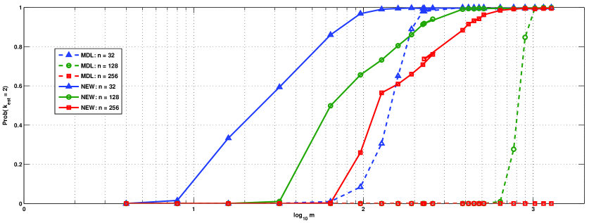
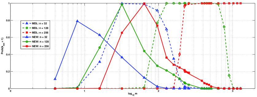
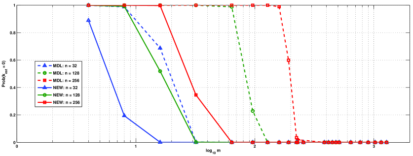
We first investigate the large sample consistency in the classical sense of $n$ fixed and $m\to\infty$. For a choice of $n$, and different values of $m$ we compute the empirical probability of detecting two signals. For large values of $m$ we expect both the new and the Wax-Kailath MDL estimator to detect both signals with high probability. Figure 5 plots the results obtained in the numerical simulations.

Figure 5(a) shows that for $n=32,128$, if $m$ is large enough then either estimator is able to detect both signals with high probability. However, the new estimator requires significantly less samples to do so than the Wax-Kailath MDL estimator.

Figure 6: The effective number of identifiable signals, computed using (34) for the values of $n$ (system size) and $m$ (sample size) considered in Figure 5 when the population covariance matrix has two signal eigenvalues $\lambda_{1}=10$ and $\lambda_{2}=3$ and $n-2$ noise eigenvalues $\lambda_{3}=\ldots=\lambda_{n}=\sigma^{2}=1$.

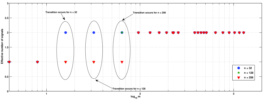
Figures 5(b) and 5(c) plot the empirical probability of detecting one and zero signals, respectively, as a function of $m$ for various values of $n$. The results exhibit the chronically reported symptom of estimators underestimating the number of signals - this is not surprising given the discussion in Section VI. Figure 6 plots the effective number of identifiable signals $k_{eff}$, determined using (34) for the various values of $n$ and $m$ considered. We observe that the values of $n$ and $m$ for which the empirical probability of the new estimator detecting one signal is high also correspond to regimes where $k_{eff}=1$. This suggests that the asymptotic concept of the effective number of signals remains relevant in a non-asymptotic regime as well. At the same time, however, one should not expect the signal identifiability/unidentifiability predictions in Section VI to be accurate in the severely sample starved settings where $m\ll n$. For example, Figure 5(c) reveals that the new estimator detects zero signals with high empirical probability when there are less than $10$ samples available even though $k_{eff}=1$ in this regime from Figure 6. In the large system, relatively large sample size asymptotic limit, however, these predictions are accurate - we discuss this next.

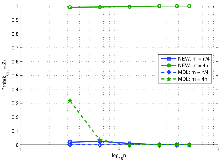
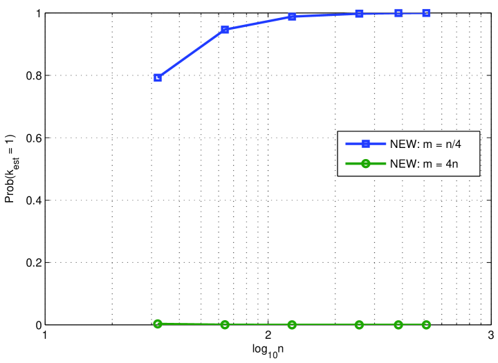
When $m=4n$ samples are available, Figure 7(a) shows that the proposed estimator consistently detects two signals while the Wax-Kailath MDL estimator does not. However, when $m=n/4$ samples are available, Figure 7(a) suggests that neither estimator is able to detect both the signals present. A closer examination of the empirical data presents a different picture. The population covariance has two signal eigenvalues $\lambda_{1}=10$ and $\lambda_{2}=3$ with the noise eigenvalues $\sigma^{2}=1$. Hence, when $m=n/4$, from (33), the effective number of signals $k_{eff}=1$. Figure 7(b) shows that for large $n$ and $m=n/4$, the new estimator consistently estimates one signal, as expected. We remark that that the signal eigenvalue $\lambda_{2}$ which is asymptotically unidentifiable falls exactly on the threshold in (33). The consistency of the new estimator with respect to the effective number of signals corroborates the asymptotic tightness of the fundamental limit of sample eigenvalue based detection. On inspecting Tables I-(b) and I-(d) it is evident that the Wax-Kailath MDL estimator consistently underestimates the effective number of signals in the large system, large sample size limit.

Table II provides additional evidence for Conjecture VI.3. We offer Tables II-(c) and II-(d) as evidence for the observation that large system, large sample consistency aside, the rate of convergence can be arbitrary slow and cannot be entirely explained by the metric $\mathcal{Z}^{{\rm SEP}}_{k_{eff}}$ in (39).

(a) Empirical probability that $\widehat{k}=2$ for various $n$ and fixed $n/m$.

(b) Empirical probability that $\widehat{k}=1$ for various $n$ and fixed $n/m$.

Figure 7: Comparison of the performance of the new estimator in (9) with the MDL estimator in (8) for various values of $n$ (system size) with $m$ (sample size) such that $n/m$ is fixed.

TABLE I: Comparison of the empirical performance of the new estimator in (9) with the Wax-Kailath MDL estimator in (8) when the population covariance matrix has two signal eigenvalues $\lambda_{1}=10$ and $\lambda_{2}=3$ and $n-2$ noise eigenvalues $\lambda_{3}=\ldots=\lambda_{n}=\sigma^{2}=1$. The effective number of identifiable signals is computed using (34) while the separation metric $\mathcal{Z}^{{\rm SEP}}_{j}$ is computed for $j=k_{eff}$ using (39). Here $n$ denotes the system size, $m$ denotes the sample size and the snapshot vectors, modelled in (1) are taken to be complex-valued.

TABLE II: Comparison of the empirical performance of the new estimator in (9) with the Wax-Kailath MDL estimator in (8) when the population covariance matrix has two signal eigenvalues $\lambda_{1}=10$ and $\lambda_{2}=3$ and $n-2$ noise eigenvalues $\lambda_{3}=\ldots=\lambda_{n}=\sigma^{2}=1$. The effective number of identifiable signals is computed using (34) while the separation metric $\mathcal{Z}^{{\rm SEP}}_{j}$ is computed for $j=k_{eff}$ using (39). Here $n$ denotes the system size, $m$ denotes the sample size and the snapshot vectors, modelled in (1) are taken to be complex-valued.

VIII Concluding remarks

We have developed an information theoretic approach for detecting the number of signals in white noise from the sample eigenvalues alone. The proposed estimator explicitly takes into account the blurring of the sample eigenvalues due to the finite size. The stated conjecture on the consistency of the algorithm, in both the $n$ fixed, $m\to\infty$ sense and the $n,m(n)\to\infty$ with $n/m(n)\to c$ sense remains to be proven. It would be interesting to investigate the impact of a broader class of penalty functions on the consistency, strong or otherwise, in both asymptotic regimes, in the spirit of [23].

In future work, we plan to address the problem of estimating the number of high-dimensional signals in noise with arbitrary covariance [24], using relatively few samples when an independent estimate of the noise sample covariance matrix, that is itself formed from relative few samples, is available. This estimator will also be of the form in 9 and will exploit the analytical characterization of properties of the traces of powers of random Wishart matrices with a covariance structure that is also random [43].

It remains an open question to analyze such signal detection algorithms in the Neyman-Pearson sense of finding the most powerful test that does not exceed a threshold probability of false detection. Finer properties, perhaps buried in the rate of convergence to the asymptotic results used, might be useful in this context. In the spirit of Wax and Kailath’s original work, we developed a procedure that did not require us to make any subjective decisions on setting threshold levels. Thus, we did not consider largest eigenvalue tests in sample starved settings of the sort developed in [44, 31] and the references therein. Nevertheless, if the performance can be significantly improved using a sequence of nested hypothesis tests, then this might be a price we might be ready to pay. This is especially true for the detection of low-level signals right around the threshold where the asymptotic results suggest that it becomes increasingly difficult, if not impossible, to detect signals using the sample eigenvalues alone.

References

- [1] J. Wishart, “The generalized product moment distribution in samples from a normal multivariate population,” Biometrika, vol. 20 A, pp. 32–52, 1928.
- [2] M. Wax and T. Kailath, “Detection of signals by information theoretic criteria,” IEEE Trans. Acoust. Speech Signal Process., vol. 33, no. 2, pp. 387–392, 1985.
- [3] K. M. Wong, Q. Zhang, J. P. Reilly, and . C. Yi, “On information theoretic criteria for determining the number of signals in high resolution array rocessing,” IEEE Trans. Acoustics, Speech, Signal Process., vol. 38, pp. 1959–1971, November 1990.
- [4] A. A. Shah and D. W. Tufts, “Determination of the dimension of a signal subspace from short data records,” IEEE Trans. Signal Process., vol. SP-42, pp. 2531–2535, September 1994.
- [5] A. P. Liavas and P. A. Regalia, “On the behavior of information theoretic criteria for model order selection,” IEEE Trans. Signal Process., vol. 49, no. 8, pp. 1689–1695, August 2001.
- [6] E. Fishler and H. Messer, “On the use of order statistics for improved detection of signals by the mdl criterion,” IEEE Trans. of Signal Process., vol. 48, no. 8, pp. 2242–2247, August 2000.
- [7] E. Fishler, M. Grossman, and H. Messer, “Detection of signals by information theoretic criteria: General asympstotic performance analysis,” IEEE Trans. Signal Process., vol. 50, no. 5, pp. 1027–1036, May 2002.
- [8] K. Johansson, “On fluctuations of random Hermitian matrices,” Duke Math. J., vol. 91, pp. 151–203, 1998.
- [9] D. Jonsson, “Some limit theorems for the eigenvalues of a sample covariance matrix,” J. of Multivar. Anal., vol. 12, pp. 1–38, 1982.
- [10] Z. D. Bai and J. W. Silverstein, “CLT for linear spectral statistics of a large dimensional sample covariance matrix,” Annals of Probability, vol. 32, pp. 553–605, 2004.
- [11] I. Dumitriu and A. Edelman, “Global spectrum fluctuations for the -Hermite and -Laguerre ensembles via matrix models,” J. Math. Phys., vol. 47, no. 6, pp. 063 302, 36, 2006.
- [12] J. Baik and J. W. Silverstein, “Eigenvalues of large sample covariance matrices of spiked population models,” Journal of Multivariate Analysis, no. 6, pp. 1382–1408, 2006.
- [13] D. Paul, “Asymptotics of sample eigenstructure for a large dimensional spiked covariance model,” Stanford University,” Technical Report, 2005, http://anson.ucdavis.edu/~debashis/techrep/eigenlimit.pdf (To appear in 2007 in Statistica Sinica).
- [14] J. Baik, G. Ben Arous, and S. Péché, “Phase transition of the largest eigenvalue for nonnull complex sample covariance matrices,” Ann. Probab., vol. 33, no. 5, pp. 1643–1697, 2005.
- [15] R. R. Nadakuditi, “Applied Stochastic Eigen-Analysis,” Ph.D. dissertation, Massachusetts Institute of Technology, February 2007, Department of Electrical Engineering and Computer Science.
- [16] M. S. Bartlett, “A note on the multiplying factors for various approximations,” J. Roy. Stat. Soc., ser. B, vol. 16, pp. 296–298, 1954.
- [17] D. N. Lawley, “Tests of significance of the latent roots of the covariance and correlation matrices,” Biometrica, vol. 43, pp. 128–136, 1956.
- [18] H. Akaike, “Information theory and an extension of the maximum likelihood principle,” in Second International Symposium on Inform. Theory (Tsahkadsor, 1971). Budapest: Akadémiai Kiadó, 1973, pp. 267–281.
- [19] ——, “A new look at the statistical model identification,” IEEE Trans. Automatic Control, vol. AC-19, pp. 716–723, 1974, system identification and time-series analysis.
- [20] G. Schwartz, “Estimating the dimension of a model,” Annals of Statistics, vol. 6, pp. 461–464, 1978.
- [21] J. Rissanen, “Modeling by shortest data description,” Automatica, vol. 14, pp. 465–471, 1978.
- [22] H. L. V. Trees, Detection, Estimation, and Modulation Theory Part IV: Optimum Array Processing. new York: John wiley and Sons, Inc., 2002.
- [23] L. C. Zhao, P. R. Krishnaiah, and Z. D. Bai, “On detection of the number of signals in presence of white noise,” J. Multivariate Anal., vol. 20, no. 1, pp. 1–25, 1986.
- [24] ——, “On detection of the number of signals when the noise covariance matrix is arbitrary,” J. Multivariate Anal., vol. 20, no. 1, pp. 26–49, 1986.
- [25] P. Stoica and M. Cedervall, “Detection tests for array procesing in unknown correlated noise fields,” IEEE Trans. Signal Process., vol. 45, pp. 2351–2362, September 1997.
- [26] E. Fishler and H. V. Poor, “Estimation of the number of sources in unbalanced arrays via information theoretic criteria,” IEEE Trans. of Signal Process., vol. 53, no. 9, pp. 3543–3553, September 2005.
- [27] A. B. Baggeroer, “Private communication.”
- [28] T. W. Anderson, “Asymptotic theory of principal component analysis,” Annals of Math. Statistics, vol. 34, pp. 122–248, 1963.
- [29] N. K. Bansal and M. Bhandary, “Bayes estimation of number of signals,” Ann. Inst. Statist. Math., vol. 43, no. 2, pp. 227–243, 1991.
- [30] J.-R. Larocque, J. P. Reilly, and W. Ng, “Particle filters for tracking and unknown number of sources,” IEEE Trans. of Signal Processing, vol. 50, no. 12, pp. 2926–2937, December 2002.
- [31] I. M. Johnstone, “High dimensional statistical inference and random matrices,” in Proc. International Congress of Mathematicians, 2006, http://arxiv.org/abs/math/0611589.
- [32] A. Edelman and N. R. Rao, “Random matrix theory,” in Acta Numerica. Cambridge University Press, 2005, vol. 14, pp. 233–297.
- [33] V. A. Marčenko and L. A. Pastur, “Distribution of eigenvalues in certain sets of random matrices,” Mat. Sb. (N.S.), vol. 72 (114), pp. 507–536, 1967.
- [34] K. W. Wachter, “The strong limits of random matrix spectra for sample matrices of independent elements,” Annals of Probab., vol. 6, pp. 1–18, 1978.
- [35] J. W. Silverstein and S.-I. Choi, “Analysis of the limiting spectral distribution of large-dimensional random matrices,” J. Multivariate Anal., vol. 54, no. 2, pp. 295–309, 1995.
- [36] J. W. Silverstein, “Strong convergence of the empirical distribution of eigenvalues of large dimensional random matrices,” J. of Multivariate Anal., vol. 55(2), pp. 331–339, 1995.
- [37] I. Dumitriu and E. Rassart, “Path counting and random matrix theory,” Electronic Journal of Combinatorics, vol. 7, no. 7, 2003, r-43.
- [38] G. Casella and R. L. Berger, Statistical inference, ser. The Wadsworth & Brooks/Cole Statistics/Probability Series. Pacific Grove, CA: Wadsworth & Brooks/Cole Advanced Books & Software, 1990.
- [39] Y. Q. Yin, Z. D. Bai, and P. R. Krishnaiah, “On the limit of the largest eigenvalue of the large-dimensional sample covariance matrix,” Probab. Theory Related Fields, vol. 78, no. 4, pp. 509–521, 1988.
- [40] J. W. Silverstein, “Private communication.”
- [41] S. Miron, N. Le Bihan, and J. Mars, “Quaternion-MUSIC for vector-sensor array processing,” IEEE Trans. on Signal Process., vol. 54, no. 4, pp. 1218–1229, April 2006.
- [42] M. Kaveh, H. Wang, and H. Hung, “On the theoretical performance of a class of estimators of the number of narrow-band sources,” IEEE Trans. Acoustics, Speech, and Signal Process., vol. ASSP-35, no. 9, pp. 1350–1352, September 1987.
- [43] N. R. Rao, J. Mingo, R. Speicher, and A. Edelman, “Statistical eigen-inference from large wishart matrices,” submitted to the Annals of Statistics. Available online at http://arxiv.org/abs/math/0701314.
- [44] I. M. Johnstone, “On the distribution of the largest eigenvalue in principal components analysis,” Annals of Statistics, vol. 29(2), pp. 295–327, 2001.