Reduced Complexity Sphere Decoding for Square QAM via a New Lattice Representation

Abstract

Sphere decoding (SD) is a low complexity maximum likelihood (ML) detection algorithm, which has been adapted for different linear channels in digital communications. The complexity of the SD has been shown to be exponential in some cases, and polynomial in others and under certain assumptions. The sphere radius and the number of nodes visited throughout the tree traversal search are the decisive factors for the complexity of the algorithm. The radius problem has been addressed and treated widely in the literature. In this paper, we propose a new structure for SD, which drastically reduces the overall complexity. The complexity is measured in terms of the floating point operations per second (FLOPS) and the number of nodes visited throughout the algorithm’s tree search. This reduction in the complexity is due to the ability of decoding the real and imaginary parts of each jointly detected symbol independently of each other, making use of the new lattice representation. We further show by simulations that the new approach achieves 80% reduction in the overall complexity compared to the conventional SD for a 2x2 system, and almost 50% reduction for the 4x4 and 6x6 cases, thus relaxing the requirements for hardware implementation.

I Introduction

Minimizing the bit error rate (BER) and thus improving the performance is the main challenge of receiver design for multiple- input multiple-output (MIMO) systems. However, the performance improvements usually come at the cost of increased complexity in the receiver design. Assuming that the receiver has perfect knowledge of the channel H, different algorithms have been implemented to separate the data streams corresponding to N transmit antennas [1]. Among these algorithms, Maximum Likelihood detection (ML) is the optimum one. However, in MIMO systems, the ML problem becomes exponential in the number of possible constellation points making the algorithm unsuitable for practical purposes [2]. Sphere decoding, on the other hand, or the Fincke-Pohst algorithm [3], reduces the computational complexity for the class of computationally hard combinatorial problems that arise in ML detection problems [4]-[5].

Complexity reduction techniques for SD have been proposed in the literature. Among these techniques, the increased radius search (IRS) [6] and the improved increasing radius search (IIRS) [7] suggested improving SD complexity efficiency by making a good choice of the sphere radius, trying to reduce the number of candidates in the search space. The former suggested a set of sphere radii ${c_{1}<c_{2}<...<c_{n}}$ such that SD starts with ${c_{1}}$ trying to find a candidate. If no candidates were found, SD executes again using the increased radius ${c_{2}}$. The algorithm continues until either a candidate is found or the radius is increased to ${c_{n}}$ which should be large enough to guarantee obtaining at least one candidate. Whereas, the latter provided a mechanism to avoid the waste of computations taking place in the former method when a certain radius ${c_{m}}$ does not lead to a candidate solution. Obviously, these two techniques studied the complexity problem from the radius choice perspective.

In this paper we improve the SD complexity efficiency by reducing the number of FLOPS required by the SD algorithm keeping in mind the importance of choosing a radius. The radius should not be too small to result in an empty sphere and thus restarting the search, and at the same time, it should not be too large to increase the number of lattice points to be searched. We use the formula presented in [8] for the radius, which is ${\textit{d}^{2}=2\sigma^{2}\textit{N}}$, where N is the problem dimension and ${\sigma^{2}}$ is the noise variance. The reduction of the number of FLOPS is accomplished by introducing a new and proper lattice representation, as well as incorporating quantization at a certain level of the SD search. It is also important to mention that searching the lattice points using this new formulation can be performed in parallel, since the new proposed structure in this paper enables decoding the real and imaginary parts of each symbol independently and at the same time.

The remainder of this paper is organized as follows: In Section II, a problem definition is introduced and a brief review of the conventional SD algorithm is presented. In Section III, we propose the new lattice representation and perform the mathematical derivations for complexity reduction. Performance and complexity comparisons for different number of antennas or modulation schemes are included in Section IV. Finally, we conclude the paper in Section V.

II Problem Definition and the Conventional Sphere Decoder

Consider a MIMO system with N transmit and M receive antennas. The received signal at each instant of time is given by

$$y=Hs+v$$ (1)

where $y\in\mathbb{C}^{\textit{M}}$, $H\in\mathbb{C}^{\textit{M}{\mathrm{x}}\textit{N}}$ is the channel matrix, $s\in\mathbb{C}^{\textit{N}}$ is an N dimensional transmitted complex vector whose entries have real and imaginary parts that are integers, $v\in\mathbb{C}^{\textit{M}}$ is the i.i.d complex additive white Gaussian noise (AWGN) vector with zero-mean and covariance matrix ${\sigma^{2}{I}}$. Usually, the elements of the vector $s$ are constrained to a finite set $\Omega$ where $\Omega\subset\mathbb{Z}^{2N}$, e.g., ${\Omega=\{-3,-1,1,3\}}^{2N}$ for 16-QAM (quadrature amplitude modulation) where $\mathbb{Z}$ and $\mathbb{C}$ denote the sets of integers and complex numbers respectively.

Assuming $H$ is known at the receiver, the ML detection is given by

$$\hat{s}=\textrm{arg}\min\limits_{s\in\Omega}{||y-Hs||}^{2}.$$ (2)

Solving (2) becomes impractical and exhaustive for high transmission rates, and the complexity grows exponentially. Therefore, instead of searching the whole space defined by all combinations drawn by the set $\Omega$, SD solves this problem by searching only over those lattice points or combinations that lie inside a sphere centered around the received vector $y$ and of radius $d$. Introducing this constraint on (2) will change the problem to

$$\hat{s}=\textrm{arg}\min\limits_{s\in\Omega}{||y-Hs||}^{2}<d^{2}.$$ (3)

A frequently used solution for the QAM-modulated complex signal model given in (3) is to decompose the $N$-dimensional problem into a 2$N$-dimensional real-valued problem, which then can be written as

$$\left[\begin{array}[]{c c}\Re\{y\}\\ \Im\{y\}\end{array}\right]=\left[\begin{array}[]{c c}\Re\{H\}&-\Im\{H\}\\ \Im\{H\}&\Re\{H\}\end{array}\right]\left[\begin{array}[]{c c}\Re\{s\}\\ \Im\{s\}\end{array}\right]+\left[\begin{array}[]{c c}\Re\{v\}\\ \Im\{v\}\end{array}\right]$$ (4)

where $\Re\{y\}$ and $\Im\{y\}$ denote the real and imaginary parts of $y$, respectively [1], [4], [8]-[9]. Assuming $N=M$ in the sequel, and introducing the QR decomposition of $H$, where R is an upper triangular matrix, and the matrix Q is unitary, (3) can be written as

$$\hat{s}=\textrm{arg}\min\limits_{s\in\Omega}{||\bar{y}-Rs||}^{2}<d^{2}$$ (5)

where $\bar{y}=Q^{H}y$. Let R=$\left[r_{i,j}\right]_{2\textit{N}\mathrm{x}2\textit{N}}$ and note that R is upper triangular. Now to solve (5), the SD algorithm constructs a tree, where the branches coming out of each node correspond to the elements drawn by the set $\Omega$. It then executes the decoding process starting with the last layer ($l=2N$) which matches the first level in the tree, calculating the partial metric $||\Im\{\bar{y}_{N}\}-r_{2N,2N}\Im\{s_{N}\}||^{2}$, and working its way up in a similar way to the successive interference cancelation technique, until decoding the first layer by calculating the corresponding partial metric $||\Re\{\bar{y}_{1}\}-r_{1,1}\Re\{s_{1}\}+...+\Re\{\bar{y}_{N}\}-r_{1,N}\Re\{s_{N}\}+\Im\{\bar{y}_{1}\}-r_{1,N+1}\Im\{s_{1}\}+...+\Im\{\bar{y}_{N}\}-r_{1,2N}\Im\{s_{N}\}||^{2}$. The summation of all partial metrics along the path of a node starting from the root constitutes the weight of that node. If that weight exceeds the square of the sphere radius $\textit{d}^{2}$, the algorithm prunes the corresponding branch, declaring it as an improbable way to a candidate solution. In other words, all nodes that lead to a solution that is outside the sphere are pruned at some level of the tree. Whenever a valid lattice point at the bottom level of the tree is found within the sphere, the square of the sphere radius $\textit{d}^{2}$ is set to the newly found point weight, thus reducing the search space for finding other candidate solutions. Finally, the leaf with the lowest weight will be the survivor one, and the path along the tree from the root to that leaf represents the estimated solution $\hat{s}$.

To this end, it is important to emphasize the fact that the complexity of this algorithm, although it is much lower than the ML detection, is still exponential at low SNR, and is directly related to the choice of the radius $d$, as well as the number of floating point operations taking place at every tree node inside the sphere.

III New Lattice Representation

The lattice representation given in (4) imposes a major restriction on the tree search algorithm. Specifically, the search has to be executed serially from one level to another on the tree. This can be made clearer by writing the partial metric weight formula as

$$w_{l}(x^{(l)})=w_{l+1}(x^{(l+1)})+|\hat{y}_{l}-\sum_{k=l}^{2N}r_{l,k}x_{k}|^{2}$$ (6)

with $l=2N,2N-1,\ldots,1$, $w_{2N+1}(x^{(2N+1)}{)=0}$ and where $\{x_{1},x_{2},...,x_{N}\}$, $\{x_{N+1},x_{N+2},...,x_{2N}\}$ are the real and imaginary parts of $\{s_{1},s_{2},...,s_{N}\}$ respectively.

Obviously, the SD algorithm starts from the upper level in the tree ($l=2N$), traversing down one level at a time, and computing the weight for one or more nodes (depending on the search strategy adopted, i.e., depth-first, breadth-first, or other reported techniques in the literature) until finding a candidate solution at the bottom level of the tree ($l=1$). According to this representation, it is impossible, for instance, to calculate $\sum_{k=l}^{2N}r_{l,k}x_{k}$ for a node in level ($l=2N-1$) without assigning an estimate for $x_{2\textit{N}}$. This approach results in two related drawbacks. First, the decoding of any $x_{\textit{l}}$ requires an estimate value for all preceding $x_{j}$ for $j=l+1,...,2N$. Secondly, there is no room for parallel computations since the structure of the tree search is sequential.

The main contribution in this paper is that we relax the tree search structure making it more flexible for parallelism, and at the same time reducing the number of computations required at each node by making the decoding of every two adjacent levels in the tree totally independent of each other.

We start by reshaping the channel matrix representation given in (4) in the following form:

$$\tilde{H}{=}\left[\begin{array}[]{c c c c c}\Re(H_{1,1})&-\Im(H_{1,1})&\cdots&\Re(H_{1,N})&-\Im(H_{1,N})\\ \Im(H_{1,1})&\Re(H_{1,1})&\cdots&\Im(H_{1,N})&\Re(H_{1,N})\\ \vdots&\vdots&\ddots&\vdots&\vdots\\ \Re(H_{N,1})&-\Im(H_{N,1})&\cdots&\Re(H_{N,N})&-\Im(H_{N,N})\\ \Im(H_{N,1})&\Re(H_{N,1})&\cdots&\Im(H_{N,N})&\Re(H_{N,N})\end{array}\right]$$ (7)

where $H_{m,n}$ is the i.i.d. complex path gain from transmit antenna $n$ to receive antenna $m$. By looking attentively at the columns of $\tilde{H}$ starting from the left hand side, and defining each pair of columns as one set, we observe that the columns in each set are orthogonal, a property that has a substantial effect on the structure of the problem. Using this channel representation changes the order of detection of the received symbols to the following form

$$\hat{y}=\left[\begin{array}[]{c c c c c}\Re(\hat{y}_{1})&\Im(\hat{y}_{1})&\cdots&\Re(\hat{y}_{N})&\Im(\hat{y}_{N})\end{array}\right]^{T}.$$ (8)

This means that the first and second levels of the search tree correspond to the real and imaginary parts of $s_{N}$, unlike the conventional SD, where those levels correspond to the imaginary part of $s_{N}$ and $s_{N-1}$ respectively. The new structure becomes advantageous after applying the QR decomposition to $\tilde{H}$. By doing so, and due to that special form of orthogonality among the columns of each set, all the elements $r_{k,k+1}$ for $k=1,3,...,2N-1$ in the upper triangular matrix R become zero. The locations of these zeros are very important since they introduce orthogonality between the real and imaginary parts of every detected symbol.

In the following, we will prove that the QR decomposition of $\tilde{H}$ introduces the aforementioned zeros. There are several methods for computing the QR decomposition, we will do so by means of the Gram-Schmidt algorithm.

Proof:

Let

$$\tilde{H}=\left[\begin{array}[]{c c c c}\mathbf{\tilde{\textbf{h}_{\textit{1}}}}&\mathbf{\tilde{\textbf{h}_{\textit{2}}}}&\cdots&\mathbf{\tilde{\textbf{h}_{\textit{2N}}}}\end{array}\right]$$ (9)

where $\mathbf{\tilde{\textbf{h}_{\textit{k}}}}$ is the $k$th column of $\tilde{\textit{H}}$. Recalling the Gram-Schmidt algorithm, we define

$\mathbf{\textbf{u}}_{\textit{1}}=\mathbf{\tilde{\textbf{h}}_{\textit{1}}}$
and then,
$\mathbf{\textbf{u}}_{\textit{k}}=\mathbf{\tilde{\textbf{h}}_{\textit{k}}}-\sum_{j=1}^{k-1}\mathrm{\phi}_{\mathbf{\textbf{u}}_{\textit{j}}}\,\mathbf{\tilde{\textbf{h}}_{\textit{k}}}$  for $k=2,3,...,2N$.
where $\mathrm{\phi}_{\mathbf{u}_{\textit{j}}}\,\mathbf{\tilde{h}_{\textit{k}}}$ is the projection of vector $\mathbf{\tilde{h}_{\textit{k}}}$ onto ${\mathbf{u}_{\textit{j}}}$ defined by

$${\mathbf{\phi}_{\mathbf{\textbf{u}}_{\textit{j}}}\,\mathbf{\tilde{\textbf{h}}_{\textit{k}}}}={\langle\mathbf{\tilde{\textbf{h}}}_{\textit{k}},\mathbf{\tilde{\textbf{u}}_{\textit{j}}}\rangle\over\langle\mathbf{\tilde{\textbf{u}}_{\textit{j}}},\mathbf{\tilde{\textbf{u}}_{\textit{j}}}\rangle}\mathbf{\tilde{\textbf{u}}_{\textit{j}}}$$ (10)

and $\mathbf{\textbf{e}}_{\textit{k}}={\mathbf{\textbf{u}}_{\textit{k}}\over\|\mathbf{\textbf{u}}_{\textit{k}}\|}$ for $k=1,2,\ldots,2N$. Rearranging the equations
$\mathbf{\tilde{h}_{\textit{1}}}=\mathbf{e}_{\textit{1}}\|\mathbf{u}_{\textit{1}}\|$
$\mathbf{\tilde{h}_{\textit{2}}}=\mathrm{\phi}_{\mathbf{u}_{\textit{1}}}\,\mathbf{\tilde{h}_{\textit{2}}}+\mathbf{e}_{\textit{2}}\|\mathbf{u}_{\textit{2}}\|$
$\mathbf{\tilde{h}_{3}}=\mathrm{\phi}_{\mathbf{u}_{\textit{1}}}\,\mathbf{\tilde{h}_{\textit{3}}}+\mathrm{\phi}_{\mathbf{e}_{\textit{2}}}\,\mathbf{\tilde{h}_{\textit{3}}}+\mathbf{e}_{\textit{3}}\|\mathbf{u}_{\textit{3}}\|$
$\vdots$
$\mathbf{\tilde{h}_{\textit{k}}}=\sum_{j=1}^{k-1}\mathrm{\phi}_{\mathbf{u}_{\textit{j}}}\,\mathbf{\tilde{h}_{\textit{k}}}+\mathbf{e}_{\textit{k}}\|\mathbf{u}_{\textit{k}}\|$.
Now, writing these equations in the matrix form, we get:

$$\left[\begin{array}[]{c c c}\mathbf{e}_{\textit{1}}&\cdots&\mathbf{e}_{\textit{n}}\end{array}\right]\left[\begin{array}[]{c c c c c}\|\mathbf{u}_{\textit{1}}\|&\langle\mathbf{e}_{\textit{1}},\mathbf{\tilde{h}_{\textit{2}}}\rangle&\langle\mathbf{e}_{\textit{1}},\mathbf{\tilde{h}_{\textit{3}}}\rangle&\ldots\\ 0&\|\mathbf{u}_{\textit{2}}\|&\langle\mathbf{e}_{\textit{2}},\mathbf{\tilde{h}_{\textit{3}}}\rangle&\ldots\\ 0&0&\|\mathbf{u}_{\textit{3}}\|&\ldots\\ \vdots&\vdots&\vdots&\ddots\end{array}\right]$$ (16)

Obviously, the matrix to the left is the orthogonal unitary Q matrix, and the one to the right is the upper triangular R matrix.
Now our task is to show that the terms $\langle\mathbf{e}_{\textit{k}},\mathbf{\tilde{h}_{\textit{k+1}}}\rangle$ are zero for $k=1,3,\ldots,2N-1$. Three observations conclude the proof.
First, since $\mathbf{\tilde{h}_{\textit{k}}}$ and $\mathbf{\tilde{h}_{\textit{k+1}}}$ are orthogonal for $k=1,3,\ldots,2N-1$, then $\mathrm{\phi}_{\mathbf{\textbf{u}}_{\textit{k}}}\,\mathbf{\tilde{\textbf{h}}_{\textit{k+1}}}$ = $\mathrm{\phi}_{\mathbf{\textbf{u}}_{\textit{k+1}}}\,\mathbf{\tilde{\textbf{h}}_{\textit{k}}}$ = 0 for the same $k$.
Second, the projection of $\mathbf{\textbf{u}}_{\textit{m}}$ for $m=1,3,\ldots,k-2$ on the columns $\mathbf{\tilde{h}_{\textit{k}}}$ and $\mathbf{\tilde{h}_{\textit{k+1}}}$ respectively is equal to the projection of $\mathbf{\textbf{u}}_{\textit{m+1}}$ on the columns $\mathbf{\tilde{h}_{\textit{k+1}}}$ and -$\mathbf{\tilde{h}_{\textit{k}}}$ respectively. To formalize this:

$$\langle\mathbf{u_{\textit{m}}},\mathbf{\tilde{h}_{\textit{k}}}\rangle=\langle\mathbf{u_{\textit{m+1}}},\mathbf{\tilde{h}_{\textit{k+1}}}\rangle$$

$$\langle\mathbf{u_{\textit{m}}},\mathbf{\tilde{h}_{\textit{k+1}}}\rangle=-\langle\mathbf{u_{\textit{m+1}}},\mathbf{\tilde{h}_{\textit{k}}}\rangle$$ (17)

for $k=1,3,\ldots,2N-1$ and $m=1,3,\ldots,k-2$. This property becomes obvious by using the first observation and revisiting the special structure of (7).
Third, making use of the first two observations, and noting that $||\mathbf{\tilde{\textbf{h}}_{\textit{k}}}||$=$||\mathbf{\tilde{\textbf{h}}_{\textit{k+1}}}||$ for $k=1,3,\ldots,2N-1$, it can be easily shown that $||\mathbf{\textbf{u}_{\textit{k}}}||$=$||\mathbf{\textbf{u}_{\textit{k+1}}}||$ for the same $k$.
Then,

$$\langle\mathbf{e}_{\textit{k}},\mathbf{\tilde{h}_{\textit{k+1}}}\rangle= {\langle{\mathbf{u}_{\textit{k}}\over\|\mathbf{u}_{\textit{k}}\|},\mathbf{\tilde{h}_{\textit{k+1}}}\rangle}$$

$$= {1\over\|\mathbf{u}_{k}\|}\langle{\mathbf{\tilde{\textbf{h}}_{\textit{k}}}-\sum_{j=1}^{k-1}\mathrm{\phi}_{\mathbf{\textbf{u}}_{\textit{j}}}\,\mathbf{\tilde{\textbf{h}}_{\textit{k}}},\mathbf{\tilde{h}_{\textit{k+1}}}\rangle}$$

$$= {1\over\|\mathbf{u}_{k}\|}({\langle{\mathbf{\tilde{\textbf{h}}_{\textit{k}}}},\mathbf{\tilde{\textbf{h}}_{\textit{k+1}}}\rangle}-{{\langle{\mathbf{\tilde{\textbf{h}}_{\textit{k}}}},\mathbf{u}_{\textit{1}}\rangle}{\langle{\mathbf{u}_{\textit{1}}},\mathbf{\tilde{\textbf{h}}_{\textit{k+1}}}\rangle}\over\langle{\mathbf{u}_{\textit{1}},\mathbf{u}_{\textit{1}}}\rangle}-$$

$${{\langle{\mathbf{\tilde{\textbf{h}}_{\textit{k}}}},\mathbf{u}_{\textit{2}}\rangle}{\langle{\mathbf{u}_{\textit{2}}},\mathbf{\tilde{\textbf{h}}_{\textit{k+1}}}\rangle}\over\langle{\mathbf{u}_{\textit{2}}},\mathbf{u}_{\textit{2}}\rangle}-\cdots-$$

$${{\langle{\mathbf{\tilde{\textbf{h}}_{\textit{k}}}},\mathbf{u}_{\textit{k-2}}\rangle}{\langle{\mathbf{u}_{\textit{k-2}}},\mathbf{\tilde{\textbf{h}}_{\textit{k+1}}}\rangle}\over\langle{\mathbf{u}_{\textit{k-1}}},\mathbf{u}_{\textit{k-1}}\rangle}-{{\langle{\mathbf{\tilde{\textbf{h}}_{\textit{k}}}},\mathbf{u}_{\textit{k-1}}\rangle}{\langle{\mathbf{u}_{\textit{k-1}}},\mathbf{\tilde{\textbf{h}}_{\textit{k+1}}}\rangle}\over\langle{\mathbf{u}_{\textit{k-2}}},\mathbf{u}_{\textit{k-2}}\rangle})$$ (18)

Now, applying the above observations to (III), we get

$$\langle\mathbf{e}_{\textit{k}},\mathbf{\tilde{h}_{\textit{k+1}}}\rangle= {1\over\|\mathbf{u}_{k}\|}(0-{{\langle{\mathbf{\tilde{\textbf{h}}_{\textit{k}}}},\mathbf{u}_{\textit{1}}\rangle}{\langle{\mathbf{u}_{\textit{1}}},\mathbf{\tilde{\textbf{h}}_{\textit{k+1}}}\rangle}\over\|\mathbf{u}_{\textit{1}}\|^{2}}-$$

$${-{\langle{\mathbf{u}_{\textit{1}}},\mathbf{\tilde{\textbf{h}}_{\textit{k+1}}}\rangle}{{\langle{\mathbf{\tilde{\textbf{h}}_{\textit{k}}}},\mathbf{u}_{\textit{1}}\rangle}}\over\|\mathbf{u}_{\textit{1}}\|^{2}}-\cdots-$$

$${{\langle{\mathbf{\tilde{\textbf{h}}_{\textit{k}}}},\mathbf{u}_{\textit{k-2}}\rangle}{\langle{\mathbf{u}_{\textit{k-2}}},\mathbf{\tilde{\textbf{h}}_{\textit{k+1}}}\rangle}\over\|\mathbf{u}_{\textit{k-1}}\|^{2}}-{-{{\langle{\mathbf{u}_{\textit{k-2}}},\mathbf{\tilde{\textbf{h}}_{\textit{k+1}}}\rangle}}{\langle{\mathbf{\tilde{\textbf{h}}_{\textit{k}}}},\mathbf{u}_{\textit{k-2}}\rangle}\over\|\mathbf{u}_{\textit{k-1}}\|^{2}})$$

$$=0$$

This concludes the proof. ∎

In this context, the SD algorithm executes in the following way. First, the partial metric weight $|\hat{y}_{2N}-r_{2N,2N}\hat{x}_{2N}|^{2}$ for the $\mu$ nodes in the first level of the tree is computed, where $\mu$ is the number of elements in $\Omega$. This metric is then checked against the specified sphere radius $d^{2}$. If the weight at any node is greater than the sphere radius then the corresponding branch is pruned. Otherwise, the metric value is saved for the next step. At the same time, another set of $\mu$ partial metric computations of the form $|\hat{y}_{2N-1}-r_{2N-1,2N-1}\hat{x}_{2N-1}|^{2}$ take place at the second level, since these two levels are independent as proved above. These metrics are checked against $d^{2}$ in a similar way to that done in the above level. The weights of the survivor nodes from both levels are summed up and the summation is checked against the sphere constraint, ending up with a set of survivor ${\hat{s}_{N}}$ symbols. Secondly, the estimation of the remaining $\hat{x}_{2N-2}$ or $\hat{s}_{N-1}$ symbols is done by quantization to the nearest constellation element in $\Omega$. In other words, the values of $\hat{x}_{2N-2},\ldots,\hat{x}_{1}$ are calculated recursively for each combination of survived $\hat{x}_{2N},\hat{x}_{2N-1}$, and the total weight given by $||\hat{y}-R\hat{s}||^{2}$ is determined at the bottom level of the tree for those leaves that obey the radius constraint. Finally, the leaf with the minimum weight is chosen to be the decoded message $(\hat{s})$. This can be formalized as
Step1:
for $i=1$ to $\mu$
$\hat{x}_{2N}=\Omega(\mu)$
$\hat{x}_{2N-1}=\Omega(\mu)$
if $|\hat{y}_{2N}-r_{2N,2N}\hat{x}_{2N}|^{2}<d^{2}$ $\rightarrow$ add to survivor set 1
else $\rightarrow$ prune branch
if $|\hat{y}_{2N-1}-r_{2N-1,2N-1}\hat{x}_{2N-1}|^{2}<d^{2}$ $\rightarrow$ add to survivor
set 2
else $\rightarrow$ prune branch
next $i$
save all combinations of $\hat{x}_{2N},\hat{x}_{2N-1}$ whose weight summations comply to the radius constraint. Denote the number of survivors at the end of this step by {$\lambda$}.
Step2: (for every combination in $\lambda$, calculate $\hat{x}_{2N-2},...,\hat{x}_{1}$ recursively as shown below)
for $l=2N-2$ to $1$, step $-2$
set $\upsilon$=$l/2$, and calculate

$$e_{l}=\sum_{\stackrel{{\scriptstyle k=l+1}}{{}}}^{2N}r_{l,k}\hat{x}_{k}, \qquad e_{l-1}=\sum_{\stackrel{{\scriptstyle k=l+1}}{{}}}^{2N}r_{l-1,k}\hat{x}_{k}$$

$$\hat{x}_{l}=\mho({\Im(\hat{y}_{\upsilon})-e_{l}\over r_{l,l}}), \qquad\hat{x}_{l-1}=\mho({\Re(\hat{y}_{\upsilon})-e_{l-1}\over r_{l-1,l-1}})$$

$$w_{l}(\hat{x}^{(l)}) =w_{l+1}(\hat{x}^{(l+1)})+|\Im{(\hat{y}_{\upsilon})}-e_{l}-\hat{x}_{l}r_{l,l}|^{2}$$

$$w_{l-1}(\hat{x}^{(l-1)}) =w_{l}(\hat{x}^{(l)})+|\Re{(\hat{y}_{\upsilon})}-e_{l-1}-\hat{x}_{l-1}r_{l-1,l-1}|^{2}$$

next $l$
where $\mho$(.) quantizes the value (.) to the closest element in the set $\Omega$. The output of the above two steps is a set of candidate solutions $\hat{x}_{2N},...,\hat{x}_{1}$ with corresponding weights.
Step3:
choose that set of $\hat{x}_{2N},...,\hat{x}_{1}$ which has the lowest weight to be the detected message.

Finally, the above algorithm’s complexity is linear with the number of antennas, and the performance is optimal for MIMO systems having two antennas at both ends. However, this performance becomes suboptimal for systems with $N\geq 3$ (e.g., there is a $4$ dB loss compared to the conventional SD at a BER of $10^{-5}$ for a 4x4 system ). This is mainly due to the use of quantization which takes place at all tree levels except the first two, and makes the estimation of $\hat{x}$s loose as we further traverse down in the tree. Thus, we introduce minor heuristic rules in the middle levels of the tree when $N\geq 3$, while still using the above steps at the very first and very last two levels in the tree, in order to obtain near optimal performance (less than $1$ dB loss), sticking with a complexity that is very much small compared to the conventional SD. A brief discussion on how to specify these rules are proposed in Section IV.

IV Simulation Results

We have considered 2x2, 4x4, and 6x6 cases using 16-QAM and 64-QAM modulation schemes. As mentioned in the previous section, we introduce heuristic rules in the middle levels of the tree when $N\geq 3$. Therefore, in our simulations for the 4x4 and 6x6 cases, we executed the algorithm in the following way:

For the 4x4 system, the first two levels of the tree which correspond to the imaginary and real parts of the symbol $\hat{s}_{4}$ are treated the same way as explained in Step 1 of the algorithm. For each survivor $\hat{s}_{4}$, the weight for all different $\mu^{2}$ possibilities of $\hat{s}_{3}$ is calculated, and those weights that violate the radius constraint are dismissed (${d^{2}=2\sigma^{2}N}$ [8]). The best 8 survivors, or in other words, those 8 $\hat{s}_{3}$’s that have lowest weights are kept for next steps while for the others the corresponding paths are pruned. In the third two levels, the same procedure performed in the previous step is applied and the best 8 $\hat{s}_{2}$’s are kept. Finally, a quantization process followed by an estimation of the transmitted message is carried out exactly the same way as in step 2 and 3 explained in the previous section. On the other hand, the 6x6 case has similar approach but with different parameters. The first two levels are treated similarly as explained in step 1. For the 16-QAM (64-QAM) case, the best 16, 8, and 4 (32,32, and 16) survivors of $\hat{s}_{6}$, $\hat{s}_{5}$, and $\hat{s}_{4}$ respectively are kept in the middle levels until reaching the last four levels which are then processed by quantization, in order to obtain $\hat{s}_{2}$ and $\hat{s}_{1}$.

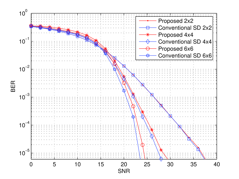
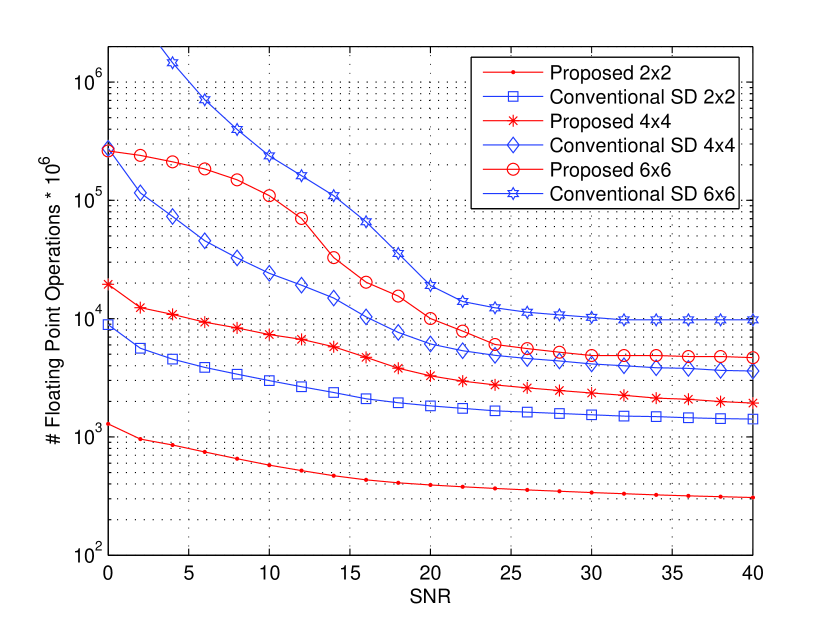
Figure 2 reports the performance of the proposed algorithm versus the conventional SD, for 2x2, 4x4, and 6x6 cases using 16-QAM modulation. We observe that the proposed algorithm achieves exactly the same performance as the conventional SD, but with much smaller complexity as shown in Figure 2. However, there is almost $0.5-1$ dB performance loss in the proposed 4x4 and 6x6 compared to the conventional. This loss is due to the $k$-best criteria adoption at a certain level of the tree as well as applying the quantization process at the low levels of the tree as mentioned above. From Figure 2, it is clear that the proposed algorithm reduces the complexity by 80% for the 2x2 case, and 50% for both the 4x4 and 6x6 systems.

Figure 1: BER vs SNR for the proposed and conventional SD over a 2x2, 4x4, and 6x6 MIMO flat fading channel using 16-QAM modulation.

Figure 2: Total number of floating point operations vs SNR for the proposed and conventional SD over a 2x2, 4x4 and 6x6 MIMO flat fading channel using 16-QAM modulation.

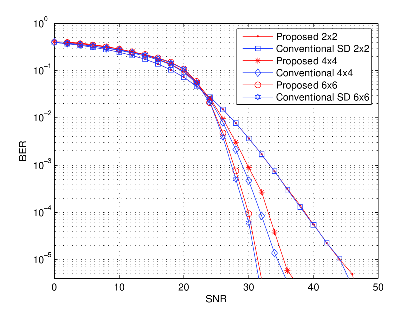
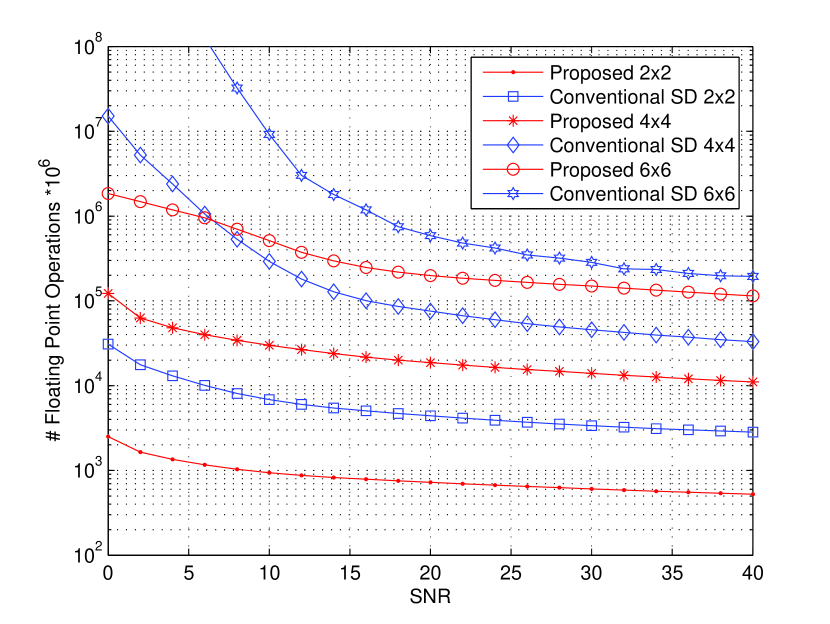
Figures 4 and 4 show the performance and complexity curves for the 2x2, 4x4, and 6x6 cases, for the 64-QAM modulation. Again, the performance is shown to be close to the conventional for the 2x2 case, and has almost $0.5-1$ dB degradation loss for the 4x4 and 6x6 cases. The difference in the complexity for the proposed and conventional SD are within the same range as in the 16-QAM modulation case.

Figure 3: BER vs SNR for the proposed and conventional SD over a 2x2, 4x4, and 6x6 MIMO flat fading channel using 64-QAM modulation.

Figure 4: Total number of floating point operations vs SNR for the proposed and conventional SD over a 2x2, 4x4, and 6x6 MIMO flat fading channel using 64-QAM modulation.

V Conclusions

A simple and general lattice representation in the context of sphere decoding was proposed in this paper. The performance of the proposed structure was shown to be optimal for 2x2 systems while close to optimal ($0.5-1$ dB loss) in the 4x4 and 6x6 cases. A complexity reduction of 80% was attainable for the 2x2 case, and 50% for the 4x4 and 6x6 cases, compared to their correspondence for the conventional SD.

References

• [1] A.ย Burg, M.ย Borgmann, M.ย Wenk, M.ย Zellweger, W.ย Fichtner, and H.ย Bolcskei, โ€œVLSI implementation of MIMO detection using the sphere decoding algorithm,โ€ IEEE Journal of Solid-State Circuits, vol.ย 40, pp. 1566โ€“1577, July 2005.
• [2] E.ย Zimmermann, W.ย Rave, and G.ย Fettweis, โ€œOn the complexity of sphere decoding,โ€ in Proc. International Symp. on Wireless Pers. Multimedia Commun., Abano Terme, Italy, Sep. 2004.
• [3] U.ย Fincke and M.Pohst, โ€œImproved methods for calculating vectors of short length in lattice, including a complexity analysis,โ€ Mathematics of Computation, vol.ย 44, pp. 463โ€“471, April 1985.
• [4] J.ย Jald n and B.ย Ottersten, โ€œOn the complexity of sphere decoding in digital communications,โ€ IEEE Trans. Signal Processing, vol.ย 53, no.ย 4, pp. 1474โ€“1484, April 2005.
• [5] B.ย Hassibi and H.ย Vikalo, โ€œOn the sphere-decoding algorithm I. Expected complexity,โ€ IEEE Trans. Signal Processing, vol.ย 53, no.ย 8, pp. 2806โ€“2818, August 2005.
• [6] E.ย Viterbo and J.ย Boutros, โ€œA universal lattice code decoder for fading channels,โ€ IEEE Trans. Inform. Theory, vol.ย 45, no.ย 5, pp. 1639โ€“1642, July 1999.
• [7] W.ย Zhao and G.ย Giannakis, โ€œSphere decoding algorithms with improved radius search,โ€ IEEE Trans. Commun., vol.ย 53, no.ย 7, pp. 1104โ€“1109, July 2005.
• [8] G.ย Rekaya and J.ย Belfiore, โ€œOn the complexity of ML lattice decoders for decoding linear full-rate space-time codes,โ€ in Proceedings 2003 IEEE International Symposium on Information Theory., July 2003.
• [9] A.ย Chan and I.ย Lee, โ€œA new reduced-complexity sphere decoder for multiple antenna systems,โ€ IEEE ICC, vol.ย 1, pp. 460โ€“464, 2002.