Ensemble inequivalence in random graphs

Abstract

We present a complete analytical solution of a system of Potts spins on a random $k$-regular graph in both the canonical and microcanonical ensembles, using the Large Deviation Cavity Method (LDCM). The solution is shown to be composed of three different branches, resulting in an non-concave entropy function.The analytical solution is confirmed with numerical Metropolis and Creutz simulations and our results clearly demonstrate the presence of a region with negative specific heat and, consequently, ensemble inequivalence between the canonical and microcanonical ensembles.

,

1 Introduction

When a system phase-separates, it pays for the different domains with a surface energy, which is usually negligible with respect to the bulk energy. As a consequence, any non concave region in the entropy vs energy curve has to be replaced by a straight line. This is the result of the usual Maxwell construction.

However, the condition of negligible surface energy is violated in presence of long range interactions, as well as for systems with a small number of components. In both cases, the possibility of non concave entropies and ensemble inequivalence is well known, and has been demonstrated on numerous models, for instance [3, 4, 7, 8]. The same condition of negligible surface energy is also violated on sparse random graphs: despite the fact that each site has only a small number of neighbors, there will be in general an extensive number of links between two (extensive) subsets of the system. The possibility of ensemble inequivalence in this type of models has been alluded to in some works related to the statistical physics of random graphs and combinatorial optimization [1]. However, these authors study the analog of the canonical ensemble, and replace the non concave part of the entropy by a straight line. This phenomenon remains thus to our knowledge unstudied, despite the widespread current interest in complex interaction structures, and networks in general. The purpose of this work is to present a simple, exactly solvable model on a random regular network, that displays a non concave entropy and ensemble inequivalence. This is a first step towards the study of more complicated networks, which may also include some local structure, like small world networks.

The paper is organized as follows: in section 2, we present the model, and give its analytical solution; we then turn in section 3 to the comparison with microcanonical simulations using both Creutz [5] microcanonical dynamics and Metropolis [6] canonical simulations. The final section is devoted to conclusions and perspectives.

2 Presentation of the model and analytical solution

2.1 The model

We study a ferromagnetic system of Potts spins with three possible states ($a$, $b$ and $c$). The Hamiltonian is chosen to be:

$$\mathcal{H}=J\sum_{\langle i,j\rangle}\left(1-\delta_{q_{i}q_{j}}\right)$$

where $\langle i,j\rangle$ denotes all the bonds in the system, $q_{i}$ is the state of spin $i$, and $\delta_{q_{i}q_{j}}$ is a Kronecker delta. In this form, the Hamiltonian simply counts the number of bonds between spins in different states. The ground state energy is $0$. The spins are located on the nodes of a regular random graph where each node has connectivity $k$, of order $1$. A mean field like version of this model, with an all-to-all coupling, has been studied by Ispolatov and Cohen [7], and displays ensemble inequivalence.

2.2 Analytical solution

Random regular graphs possess very few loops of size order $1$, and locally look like trees; this feature allows us to use standard statistical physics methods, originally developed for Bethe lattices. These calculations are usually done in the canonical ensemble only; in contrast, we are interested also in the microcanonical solution. We compute here the free energy and the entropy of the system, by following the formalism of the Large Deviation Cavity Method described by O. Rivoire in [2]. We consider however only large deviation functions with respect to spin disorder, and not with respect to disorder in the graph structure like in [2].

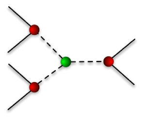
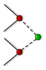
Figure 1: Schematic representation of the iteration (left), link addition (center) and site addition (right).Red nodes and solid edges represent the original cavity spins and links, while the green colored nodes and dashed lines identify the additions.

We call cavity sites sites which have only $k-1$ neighbors, and one free link. Cavity site $i$ sends a field $h_{i}$ along each link, which tells its state $a$, $b$ or $c$. These field are distributed according to the probability distribution $P\left(h\right)$:

$$P\left(h\right)=p_{a}\delta_{h,a}+p_{b}\delta_{h,b}+p_{c}\delta_{h,c}~{}.$$ (1)

$h_{0}$	$\left(h_{1},h_{2}\right)$	$\Delta E_{n}$	$prob$
	$\left(a,a\right)$	$0$	$\frac{1}{3}p_{a}^{2}$
	$\left(a,b\right)$	$1$	$\frac{1}{3}2p_{a}p_{b}$
$a$	$\left(a,c\right)$	$1$	$\frac{1}{3}2p_{a}p_{c}$
	$\left(b,b\right)$	$2$	$\frac{1}{3}p_{b}^{2}$
	$\left(b,c\right)$	$2$	$\frac{1}{3}2p_{b}p_{c}$
	$\left(c,c\right)$	$2$	$\frac{1}{3}p_{c}^{2}$
	$\left(b,b\right)$	$0$	$\frac{1}{3}p_{b}^{2}$
	$\left(b,a\right)$	$1$	$\frac{1}{3}2p_{b}p_{a}$
$b$	$\left(b,c\right)$	$1$	$\frac{1}{3}2p_{b}p_{c}$
	$\left(a,a\right)$	$2$	$\frac{1}{3}p_{a}^{2}$
	$\left(a,c\right)$	$2$	$\frac{1}{3}2p_{a}p_{c}$
	$\left(c,c\right)$	$2$	$\frac{1}{3}p_{c}^{2}$
	$\left(c,c\right)$	$0$	$\frac{1}{3}p_{c}^{2}$
	$\left(c,a\right)$	$1$	$\frac{1}{3}2p_{c}p_{a}$
$c$	$\left(c,b\right)$	$1$	$\frac{1}{3}2p_{c}p_{b}$
	$\left(a,a\right)$	$2$	$\frac{1}{3}p_{a}^{2}$
	$\left(a,b\right)$	$2$	$\frac{1}{3}2p_{a}p_{b}$
	$\left(b,b\right)$	$2$	$\frac{1}{3}p_{b}^{2}$

Table 1: Analysis of the iteration process for $k=3$: energy shifts and probabilities. $h_{0}$ is the field sent by the new cavity site.

The first step is to obtain a self consistent equation for the probabilities $p_{a},~{}p_{b}$ and $p_{c}$ through the analysis of the “iteration” process, represented on the left side of Fig 1. During an iteration step, a new site is connected to $k-1$ cavity sites to become a new cavity site. Several possibilities must be accounted for, corresponding to all the possible configurations along the newly created edges. Let us note that for infinite temperature, or $\beta=0$, each new spin has probability $1/3$ to be in each of the three states $a$, $b$ and $c$. This is the origin of the $1/3$ factors in table 1 where we represent all the terms to be considered in the $k=3$ case.

Using this table and following [2], we obtain:

$$\left\{\begin{array}[]{l}p_{a}=\frac{1}{Z}\frac{1}{3}\left\{p_{a}^{2}+2p_{a}\left(p_{b}+p_{c}\right)e^{-\beta}+\left(p_{b}+p_{c}\right)^{2}e^{-2\beta}\right\}\\ p_{b}=\frac{1}{Z}\frac{1}{3}\left\{p_{b}^{2}+2p_{b}\left(p_{a}+p_{c}\right)e^{-\beta}+\left(p_{a}+p_{c}\right)^{2}e^{-2\beta}\right\}\\ p_{c}=\frac{1}{Z}\frac{1}{3}\left\{p_{c}^{2}+2p_{c}\left(p_{a}+p_{b}\right)e^{-\beta}+\left(p_{a}+p_{b}\right)^{2}e^{-2\beta}\right\}\\ Z=\frac{1}{3}\left\{\left[p_{a}+\left(p_{b}+p_{c}\right)e^{-\beta}\right]^{2}+\left[p_{b}+\left(p_{a}+p_{c}\right)e^{-\beta}\right]^{2}+\left[p_{c}+\left(p_{a}+p_{b}\right)e^{-\beta}\right]^{2}\right\}\end{array}\right.$$ (2)

from where we can easily calculate numerically $p_{a,b,c}$. For larger $k$ the generalization is straightforward, we have:

$$p_{a}=\frac{1}{3Z}\left[p_{a}+\left(p_{b}+p_{c}\right)e^{-\beta}\right]^{k-1}$$ (3)

We compute the generalized free energy $\mathcal{F}\left(\beta\right)$ through the formula:

$$\mathcal{F}\left(\beta\right)=-\ln\left[\langle e^{-\beta\Delta E_{site}}\rangle\right]+\frac{k}{2}\ln\left[\langle e^{-\beta\Delta E_{link}}\rangle\right]~{}.$$ (4)

where $\Delta E_{site}$ and $\Delta E_{link}$ are the energy shifts due to a site and a link addition respectively. The $\langle~{}.~{}\rangle$ symbol denotes the expected value. Link and site additions are depicted on the center and right sides of Fig. 1, respectively. The analysis of the energy shifts in the $k=3$ case is detailed in Tables. 2 and 3.

$\left(h_{1},h_{2}\right)$	$\Delta E$	proba.	$P_{l}\left(\Delta E\right)$
$\left(a,a\right)$	$0$	$p_{a}^{2}$
$\left(b,b\right)$	$0$	$p_{b}^{2}$	$p_{a}^{2}+p_{b}^{2}+p_{c}^{2}$
$\left(c,c\right)$	$0$	$p_{c}^{2}$
$\left(a,b\right)$	$1$	$2p_{a}p_{b}$
$\left(a,c\right)$	$1$	$2p_{a}p_{c}$	$2\left(p_{a}p_{b}+p_{a}p_{c}+p_{b}p_{c}\right)$
$\left(b,c\right)$	$1$	$2p_{b}p_{c}$

Table 2: Configurations $\left(h_{1},h_{2}\right)$, energy shifts $\Delta E$ and total probabilities $P_{l}\left(\Delta E\right)$ for the case of a link addition. The numeric factors stem from combinatoric arguments.

new site	$\left(h_{1},h_{2},h_{3}\right)$	$\Delta E$	$P_{n}\left(\Delta E\right)$
	$\left(a,a,a\right)$	$0$	$\frac{1}{3}p_{a}^{3}$
$a$	$\left(a,a,b\right),\left(a,a,c\right)$	$1$	$\frac{1}{3}\left(3p_{a}^{2}p_{b}+3p_{a}^{2}p_{c}\right)$
	$\left(a,b,b\right),\left(a,b,c\right),\left(a,c,c\right)$	$2$	$\frac{1}{3}\left(3p_{a}p_{b}^{2}+3p_{a}p_{c}^{2}+6p_{a}p_{b}p_{c}\right)$
	$\left(b,b,b\right),\left(b,b,c\right),\left(b,c,c\right),\left(c,c,c\right)$	$3$	$\frac{1}{3}\left(p_{b}^{3}+p_{c}^{3}+3p_{b}p_{c}^{2}+3p_{c}p_{b}^{2}\right)$
	$\left(b,b,b\right)$	$0$	$\frac{1}{3}p_{b}^{3}$
$b$	$\left(b,b,a\right),\left(b,b,c\right)$	$1$	$\frac{1}{3}\left(3p_{b}^{2}p_{a}+3p_{b}^{2}p_{c}\right)$
	$\left(b,a,a\right),\left(b,a,c\right),\left(b,c,c\right)$	$2$	$\frac{1}{3}\left(3p_{b}p_{a}^{2}+3p_{b}p_{c}^{2}+6p_{b}p_{a}p_{c}\right)$
	$\left(a,a,a\right),\left(a,a,c\right),\left(a,c,c\right),\left(c,c,c\right)$	$3$	$\frac{1}{3}\left(p_{a}^{3}+p_{c}^{3}+3p_{a}p_{c}^{2}+3p_{c}p_{a}^{2}\right)$
	$\left(c,c,c\right)$	$0$	$\frac{1}{3}p_{c}^{3}$
$c$	$\left(c,c,b\right),\left(c,c,a\right)$	$1$	$\frac{1}{3}\left(3p_{c}^{2}p_{b}+3p_{c}^{2}p_{a}\right)$
	$\left(c,b,b\right),\left(c,b,a\right),\left(c,a,a\right)$	$2$	$\frac{1}{3}\left(3p_{c}p_{b}^{2}+3p_{c}p_{a}^{2}+6p_{c}p_{b}p_{a}\right)$
	$\left(b,b,b\right),\left(b,b,a\right),\left(b,a,a\right),\left(a,a,a\right)$	$3$	$\frac{1}{3}\left(p_{b}^{3}+p_{a}^{3}+3p_{b}p_{a}^{2}+3p_{a}p_{b}^{2}\right)$

Table 3: Possible configurations $\left(h_{1},h_{2},h_{3}\right)$, energy shifts $\Delta E$ and probabilities for the different states in which the new site can be. The overall factor of $\frac{1}{3}$ corresponds to the a priori probability that the new site is in state $a$ and the remaining numeric multipliers stem from combinatorics.

Plugging all the previous results in to Eq. 4, we obtain the expression of the generalized free energy of the system for the general $k$ case:

$$\mathcal{F}\left(\beta\right) = -\ln\left[\left(p_{a}^{2}+p_{b}^{2}+p_{c}^{2}\right)+2\left(p_{a}p_{b}+p_{a}p_{c}+p_{b}p_{c}\right)e^{-\beta}\right]+$$

$$+\frac{k}{2}\ln\left[\frac{1}{3}\left\{\left[p_{a}+\left(p_{b}+p_{c}\right)e^{-\beta}\right]^{k}+\right.\right.$$

$$+\left.\left.\left[p_{b}+\left(p_{a}+p_{c}\right)e^{-\beta}\right]^{k}+\left[p_{c}+\left(p_{a}+p_{b}\right)e^{-\beta}\right]^{k}\right\}\right]$$

where the three densities $p_{a}$, $p_{b}$ and $p_{c}$ are solutions of Eq. 3. Notice that this procedure does not necessarily yield a unique “free energy” $\mathcal{F}\left(\beta\right)$; rather, there is one value of $\mathcal{F}(\beta)$ for each solution of the consistency equation (3). We must then follow all branches of the multi-valued function $\mathcal{F}\left(\beta\right)$ to reconstruct the entropy $S\left(e\right)$ through a generalized inverse Legendre transform (see for instance [9] for a use of this procedure in the context of signal processing):

$$S\left(e\right)=\beta e-\mathcal{F}\left(\beta\right)$$ (6)

where:

$$e\equiv\frac{\partial\mathcal{F}}{\partial\beta}$$

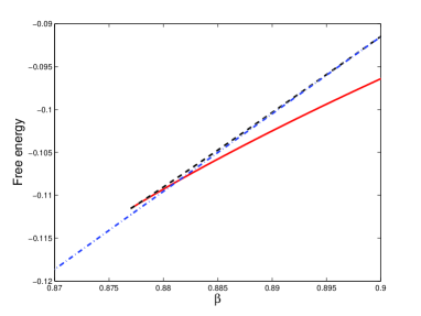
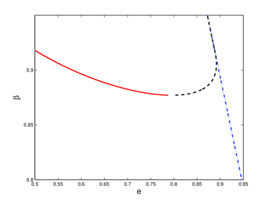
can easily be calculated numerically using finite differences. This is the final, implicit, solution for the entropy $S\left(e\right)$. In fig. 2, we plot the different solution branches of $\mathcal{F}(\beta)$, and the inverse temperature $\beta\left(e\right)$. One clearly sees a negative specific heat region, signaled by the presence of multiple function values for the same energy.

Figure 2: Left: the three branches of the generalized free energy $\mathcal{F}$ as a function of the inverse temperature $\beta$, for $k=4$. Right: the corresponding three branches for $\beta\left(e\right)$ in the microcanonical ensemble.

3 Comparison with numerical simulations

In this section we compare the analytical solution with the results obtained through numerical simulations. Microcanonical simulations were performed using Creutz [5] dynamics. During which, a fictitious “demon” is introduced, carrying an energy $e_{demon}$. At each step, a spin flip in the system is attempted, and the corresponding energy change $\delta E$ is computed. If $\delta E<0$, the move is accepted; if $\delta E>0$, the move is accepted only if $e_{demon}\geq\delta E$. In both cases $e_{demon}$ is then updated so that the total energy $E+e_{demon}$ is kept constant; the energy of the system $E$ is then constant up to a $O(1/N)$. For long run times, the demon’s energy reaches an exponential distribution $P(e_{demon}=e)\propto\exp(-e/T_{\mu})$, from where one can compute the corresponding microcanonical temperature $T_{\mu}=1/\beta_{mu}$ of our system:

$$\beta_{\mu}=\log\left[1+\frac{1}{\langle e_{demon}\rangle}\right]~{}.$$ (7)

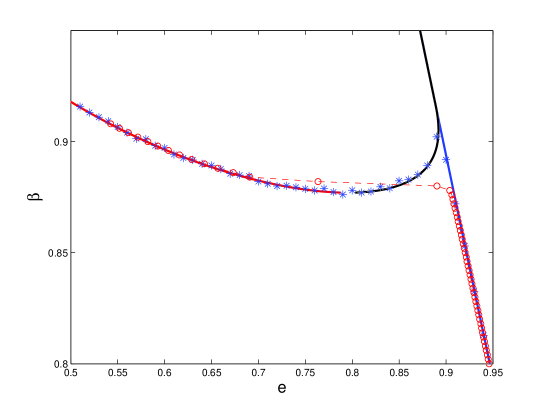
Results of the Creutz dynamics are plotted on Fig. 3 and compared with the analytical solution of the previous section. The agreement between the two is very good, with the $\beta$ vs energy curve clearly showing a region of negative specific heat.

Finally, we performed canonical Metropolis[6] simulations and calculated the average energy in the temperature range where our results predict ensemble inequivalence. As expected, the canonical caloric curve obeys Maxwell’s construction and clearly “jumps over” the region where the specific heat is negative.

Figure 3: Comparison for the caloric curve $\beta\left(e\right)$ between the analytical solution (solid lines), the Creutz dynamics results (stars), and the Metropolis simulations (circles) for $k=4$. The Creutz simulations were performed on networks with $N=40000$ sites, for $10^{8}$ “Creutz steps”, and the results were averaged over $20$ network realizations. The Metropolis results were obtained using $50$ different networks with $N=10000$ nodes, by performing $10^{10}$ Monte-Carlo steps. In both cases, the size of the error bars is comparable to the size of the symbols.

4 Conclusion and perspectives

We have presented a complete canonical and microcanonical solution of the 3-states Potts model on $k$-regular random graphs, and shown that this toy model displays ensemble inequivalence.

There is little doubt that this result should generically apply to models on different types of random graphs, such as Erdös-Rényi ones, among others. We also expect to observe ensemble inequivalence on small world networks, since in these systems, the presence of random long-range links should prevent the system from separating in two different phases.

Beyond the inequivalence between microcanonical and canonical statistical ensemble, non concave large deviation functions should be expected for some properties on random graphs. Fig. 4 of [1] gives an example of this. The present work provides an example where the Large Deviation Cavity method allows to deal with such a situation, and to compute the non concave part of the large deviation function.

References

• [1] A. Engel, R. Monasson, A. Hartmann “On Large Deviation Properties of Erdös-Rényi Random Graphs”, J. Stat. Phys 117 (2004), 387.
• [2] O. Rivoire “The cavity method for large deviations”, J. Stat. Mech. P07004 (2005).
• [3] P. Hertel, W. Thirring “Soluble model for a system with negative specific heat” Ann. Phys. 63 (1971), 520.
• [4] D. H. E. Gross Microcanonical Thermodynamics: Phase Transitions in Small Systems, Lecture Notes in Physics 66, World Scientific, Singapore (2001).
• [5] M. Creutz “Microcanonical Monte Carlo Simulation”, Phys. Rev. Lett. 50 (1983), 1411.
• [6] N. Metropolis, A. W. Rosenbluth, M. N. Rosenbluth, A. H. Teller and E. Teller “Equation of state calculations by fast computing machines” J. Chem. Phys., 21 (1953), 1087.
• [7] I. Ispolatov, E. G. D. Cohen “On first-order phase transitions in microcanonical and canonical non-extensive systems”, Physica A 295 (2001), 475.
• [8] J. Barré, D. Mukamel, S. Ruffo, “Inequivalence of ensembles in a system with long range interactions”, Phys. Rev. Lett. 87 (2001), 030601.
• [9] P. Maragos “Slope transforms: theory and applications to non linear signal processing”, IEEE Trans. Signal. Proc. 43 (1995), 864.