Towards a library of synthetic galaxy spectra and preliminary results of classification and parametrization of unresolved galaxies for Gaia

Abstract

Aims. The Gaia astrometric survey mission will, as a consequence of its scanning law, obtain low resolution optical (330–1000 nm) spectrophotometry of several million unresolved galaxies brighter than V=22. We present the first steps in a project to design and implement a classification system for these data. The goal is both to determine morphological classes and to estimate intrinsic astrophysical parameters via synthetic templates. Here we describe (1) a new library of synthetic galaxy spectra, and (2) first results of classification and parametrization experiments using simulated Gaia spectrophotometry of this library.

Methods. We have created a large grid of synthetic galaxy spectra using the PÉGASE.2 code, which is based on galaxy evolution models that take into account metallicity evolution, extinction correction, emission lines (with stellar spectra based on the BaSeL library). Our classification and regression models are Support Vector Machines (SVMs), which are kernel-based nonlinear estimators.

Results. We produce a basic library of about 3600 zero redshift galaxy spectra covering the main Hubble types over wavelength range 250 to 1050 nm at a sampling of 1 nm or less. It is computed on a regular grid of four key astrophysical parameters for each type and for intermediate random values of the same parameters. An extended library reproduces this at a series of redshifts. Initial results from the SVM classifiers and parametrizers are promising, indicating that Hubble types can be reliably predicted and several parameters estimated with low bias and variance. Comparing the colours of our synthetic library with Sloan Digital Sky Survey (SDSS) spectra we find good agreement over the full range of Hubble types and parameters.

1 Introduction

Large surveys of galaxies provide information on their global spatial distribution and the physical properties of individual galaxies. Such a survey will be obtained for the whole sky by the ESA mission, Gaia, from 2011–2016. During its five year mission Gaia will observe several million unresolved galaxies all over the whole sky. Although the survey’s main goal is the stellar content and the structure of our galaxy, there remains a lot of important science to be extracted from the galactic component.

There currently exist several surveys of galaxies, but even SDSS – one of the most extended galaxy photometric and spectroscopic surveys in the the optical and near IR (about at the spectral range of Gaia) – covers only a fifth of the sky. Gaia extends this in several ways: i) It will be able to detect about 10⁷ unresolved galaxies down to G=20 (V=20–22); ii) Gaia will be the first homogeneous survey of galaxies covering the whole sky since photographic ones (UK, ESO, Palomar Schmidt surveys, 3500 to 6500 Å) of 30 years ago; iii) The spectrophotometry covers a larger spectral range (3300 to 10 000 Å sampled in about 100 bins) than earlier surveys; iv) Gaia observes each source an average of 80 times over the mission. With this we can investigate many different types of galaxy, QSO and AGN variability; v) The sample will have a well-defined selection function, important for estimating the galaxy density in the local universe.

Our long-term objective is to classify and to determine the astrophysical parameters of all unresolved galaxies which Gaia will observe. In order to proceed with this we first need to acquire or build an appropriate library of galaxy spectra. This library must show sufficient variation in those intrinsic astrophysical parameters (APs) to which the Gaia observations will be sensitive. To determine APs on a homogeneous system we ultimately need to build or calibrate our classifiers using synthesis models and synthetic spectra. Existing observed or synthetic libraries are too small or don’t cover the required wavelength range. For this reason we set on in this paper to start building a new library.

We use the galaxy evolution model PÉGASE (Projet d’ Etude des Galaxies par Synthese Evolutive) (Fioc & Rocca-Volmerange 1997, 1999c), to synthesize galaxy spectra. The PÉGASE.2 code is aimed principally at modelling the spectral evolution of galaxies by types: the active and passive evolution of stellar populations as well as interstellar gas and dust are coherently evolved in time. No galaxy number density evolution is considered, although the results of our models are compatible with occasional rare galaxy merging. The code is based on the stellar evolutionary tracks from the Padova group, extended to the thermally pulsating asymptotic giant branch (AGB) and post-AGB phases (Groenewegen & de Jong 1993). These tracks cover all the masses, metalicities and phases of interest for galaxy spectral synthesis. PÉGASE.2 uses the BaSeL 2.2 library of stellar spectra and can synthesize low resolution (R=200) ultraviolet to near-infrared spectra of Hubble sequence galaxies, as well as of starbursts. For a given evolutionary scenario (typically characterized by a star formation law, an initial mass function and, possibly, infall or galactic winds), the code consistently gives the spectral energy distribution (SED) and computes the star formation rate and the metallicity at any time. The nebular component (continuum and lines) due to HII regions is calculated and added to the stellar component. Depending on the geometry of the galaxy (disk or spheroidal), the attenuation of the spectrum by dust is then computed using a radiative transfer code (which takes account of the scattering).

By accepting a star formation rate proportional to mass of the gas, the IMF of Rana & Basu (1992) and the presence of infall and galactic winds, eight synthetic spectra corresponding to different typical types of Hubble sequence galaxies (E, S0, Sa, Sb, Sbc, Sc, Sd and Im) have already been produced using PÉGASE.2 (Fioc 1997; Fioc & Rocca-Volmerange 1999a; Le Borgne & Rocca-Volmerange 2002). For each type, the values of the parameter set have been fitted to the observed spectral energy distribution (SED) of nearby (z=0) galaxies. For illustration a comparison with data is shown in Fioc (1999). At higher redshifts, the evolution scenarios have been tested against most existing faint galaxy samples, including the deepest surveys (B=29 Hubble Deep Field-N, Williams et al. 1996). One unique model of galaxy fractions by type simultaneously predicts the multi-wavelength (UV to near-IR) galaxy counts, dominated by young stellar populations in the UV and old evolved galaxies in the near-IR respectively. The faint blue galaxy population, in excess in the far-UV, has also been analysed (Fioc & Rocca-Volmerange 1999b). An episodic star formation rate of low level is proposed to fit the far-UV counts (Armand & Milliard 1994; Buat et al. 1999). In the near-IR, the evolution scenario of elliptical galaxies predicts the puzzling $K$-$z$ relation of radio galaxy hosts between z=0 and z=4. Rocca-Volmerange et al. (2004) use PÉGASE.2 scenarios to interpret the galaxy distribution in the K-band Hubble diagram. The same models are used to interpret the mid-IR galaxy counts (Rocca-Volmerange et al. 2007), although here a supplementary ultra-luminous infrared galaxy population is required. Finally, the robustness of our evolution scenarios is confirmed by the significant predictions of photometric redshifts as compared to spectroscopic redshifts of HDF-N sample (Le Borgne & Rocca-Volmerange 2002). Using a much larger sample from the SDSS, we make an additional comparison. This is the subject of the second section of this paper, made using simulated photometry and colour-colour diagrams. In section 3 we describe the production of our library based on these eight typical synthetic spectra of galaxies and in section 4 we explain how these are used to simulate Gaia data. In section 5 we present our classification and parametrization models and give preliminary results on their performance. A brief discussion follows in section 6.

2 PÉGASE synthetic spectra and comparison with the SDSS spectra

In order to determine the parameter ranges over which we should generate the library, we first make a comparison of colours synthesized from the eight typical PÉGASE spectra with SDSS data. To avoid small discrepancies that occur between synthesized and published SDSS photometry and to treat both types of spectral data in the same way, we decided to synthesize SDSS photometry from the SDSS spectra in the same way as we do with the synthetic spectra (and using the same “calib” and “colors” programs in the PÉGASE.2 code for both). For this we use the whole set of spectroscopic data for the 565 715 galaxies that are available in data release 4 (DR4) of SDSS. The properties of the SDSS filters are given in Table 1.

Table 1: Characteristics of the five SDSS filters

Name	Average	Starting	Ending	magnitude
	wavelength	wavelength	wavelength	limit in
	($\AA$)	($\AA$)	($\AA$)	survey
u	3551	2980	4130	22.0
g	4686	3630	5830	22.2
r	6165	5380	7230	22.2
i	7481	6430	8630	21.3
z	8931	7730	11230	20.5

Typical synthetic spectra corresponding to each of the eight Hubble types are shown in Fig. 1, with the location of the SDSS filters superimposed. Each of these “typical spectra” corresponds to specific combination of values of the astrophysical parameters (see section 3.1). The SEDs produced by PÉGASE have been normalized to the flux of a 50$\AA$ wavelength interval centered on 5500$\AA$. The elliptical and S0 galaxies have very small differences, apparent at the two extremes of the wavelength range. This implies small differences in colours but not necessarily in magnitudes (which depend on their masses).

From Fig. 1 it is obvious that the u filter is very important for the comparison with real data since it is the one containing the discontinuity around 4000$\AA$. However, the SDSS spectra do not cover the u band, so photometry in this band cannot be synthesized. We refrain from using the SDSS photometry for the u band because of the red leak in this filter, which would render comparisons with synthetic data unreliable. This leak produces erroneous magnitudes, especially for E and S0 types on account of their large numbers of red stars.

In addition we avoid using the z filter in our comparison since its photometry also cannot be synthesized from the SDSS spectra, which terminate at shorter wavelengths than the z passband.

Figure 1: Synthetic spectra for the eight typical galaxy types from PÉGASE.2. The vertical lines denote the limits of the five SDSS filters (transmission below 1e-4 of the peak). (Emission lines are not included). The legend at the right defines colour used to plot each type of galaxy (top) and SDSS filter (bottom).

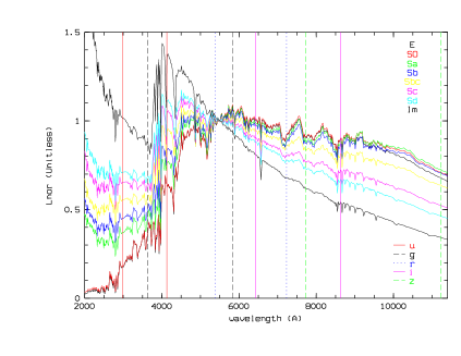
We therefore decided to base our comparison between the SDSS and PÉGASE.2 data using the g, r, i filters only and, more specifically, the g–r and r–i colours. However, the wavelength range of the SDSS spectra does not quite extend to the bluest side of the g filter. For this reason, we cut the blue end of this and created a new g filter starting at 3830$\AA$ instead of the 3630$\AA$ (table 1). However, this change is in practice very small since the transmission of the g filter is only 3% of the peak transmission at 3830$\AA$ and drops very rapidly below that (e.g. it is only 0.5% at just 10Å lower). Furthermore, simulated photometry from the synthetic spectra showed virtually no difference for the original and “trimmed” g band. The published transmission curves of the SDSS filters depend on airmass and whether a point or extended source is being observed. We use those for extended sources and zero airmass. The photometry is calibrated on the AB system, as used by SDSS (Fukugita et al. 1996).

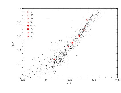
We synthesize photometry using the one-dimensional spectra from DR4, which are supplied with additional analysis information, such as redshift and emission line parameters. In order to select data suitable for our purposes, we applied the following criteria: the galaxies should not be near a CCD edge nor saturated, and they should not be very low SNR (the photometric error in all bands should be less than 0.1 mag). Only spectra with redshifts below 0.01 are retained, since the synthetic spectra of PÉGASE.2 were produced at zero redshift. These criteria resulted in a sample of 1292 galaxies. Their synthesized photometry plus that for the eight typical galaxy types from PÉGASE.2 is shown in Fig. 2. This figure clearly shows that the colours of the Im, Sd, Sc, Sbc, Sb and Sa types are generally in good agreement with the colours of the observed spectra, although in the case of S0 and E types the synthetic spectra seem to be slightly redder in g$-$r than the SDSS spectra.

Figure 2: Colour–colour (g$-$r vs. r$-$i) diagram of synthesized photometry of SDSS galaxy spectra (black) and synthetic photometry of the eight typical galaxy types generated from the PÉGASE models (red points).

3 The library of synthetic spectra

3.1 The most significant parameters

Each spectrum in our library is uniquely defined by a set of 17 astrophysical parameters, plus the morphological type (E, S0, Sa, Sb, Sbc, Sc, Sd or Im). The four most significant APs are: p1 and p2 of the star formation scenario (($Mgas^{p_{1}}$)/p2); the infall timescale; the age of the galactic winds. The age of the galactic winds is non-zero only for E and S0 galaxies. Note that the Hubble type is not an independent parameter, as only certain ranges of the APs are available for each type (as will be detailed later).

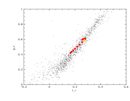
In order to investigate the influence of each of the parameters p1, p2 and infall timescale to the integrated galaxy spectrum (SED), we modified the parameters of the Sbc model (an intermediate type) over a range of values. In the typical model for the Sbc type the values were 1, 5714 Myr/$M_{\odot}$ and 6000 Myr for p1, p2 and infall timescale, respectively. In the modified models we vary p1 between 0.4 and 2, p2 from 100 to 20000 Myr/$M_{\odot}$ and infall from 100 to 10000 Myr. The results are shown in Figs. 3–5.

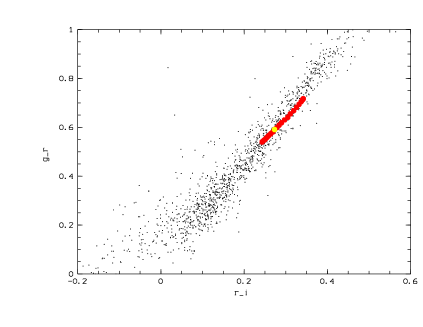
To investigate the effect of the age of the galactic winds parameter we followed the same procedure but now with the elliptical model. In the typical model for the E type the age is 1 Gyr and we vary it between 0.1 and 7.5 Gyr (Fig. 6).

From the figures we see that these four parameters have a major effect on the colours. We performed similar analyses for other APs and concluded that they had a much smaller impact on the data (in particular once the spectra are reduced to the Gaia resolution). Therefore, the spectra in the present library show variance only in these four APs.

Figure 3: Colour–colour (g–r vs r–i) diagram of synthesized photometry of SDSS galaxy spectra (black) and of synthetic PÉGASE spectra of the typical Sbc model (yellow) and the models of Sbc with different values of p1 (red). The largest g–r corresponds to p1=1 and the smallest g–r to p1=2.

Figure 4: Colour-colour (g–r vs r–i) diagram of synthesized photometry of SDSS galaxy spectra (black) and of synthetic PÉGASE spectra of the typical Sbc model (yellow) and the models of Sbc with different values of p2 (red). The largest g–r corresponds to p2=2000 Myr/$M_{\odot}$ and the smallest g–r to p2=20000 Myr/$M_{\odot}$.

Figure 5: Colour–colour (g–r vs r–i) diagram of synthesized photometry of SDSS galaxy spectra (black) and of synthetic PÉGASE spectra of the typical Sbc model (yellow) and the models of Sbc with different values of infall timescale (red). The largest g–r corresponds to infall timescale=100My and the smallest g–r to infall timescale=10 Gyr.

Figure 6: Colour–colour (g–r vs r–i) diagram of synthesized photometry of SDSS galaxy spectra (black) and of synthetic PÉGASE spectra of the typical E model (yellow) and the models of E with different values of age of galactic winds (red). The largest g–r corresponds to age of galactic winds=7.5Gy and the smallest g–r to 0.1 Gyr.

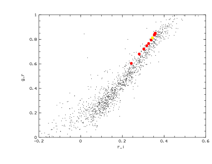
By co-varying these four parameters and using all their combinations in each of the eight typical models we are able to cover most of the variance we see in the SDSS data in the colour–colour diagram. Generally, there is no clear distinction between the colours of neighbouring Hubble types. In order to have a knowledge of types in our library we decided (as a first working approximation) to only retain those models which lie within a circle (in the colour-colour diagram) centered on one of the eight typical types and with a radius equal to half of the distance to the nearest neighbouring typical model. This is reasonable since the models lie mostly on a one-dimensional surface (line) in the colour–colour diagram. In this way upper and lower limits of the values of the parameters were established for each type, although in this case an overlap in APs (if not in colours) remains, as can be seen in table 2. This leaves a set of 888 synthetic spectra of known types of galaxies (see section 3.2).

The galaxy type can be considered as a 5th AP, although it is of a different nature than the others, since it is needed to fully specify the spectrum and constrain the range of values of the other four APs. In addition, when one redshifts the spectrum to non-zero values of z, this quantity also becomes a parameter (albeit not intrinsic to the source).

3.2 Library of galaxy spectra over a regular grid of parameters

Applying the above procedures, we produced a library of 888 synthetic spectra covering seven separate Hubble types (because we consider E and S0 as a single type). The values of the four parameters of each type are given in table 2, while the values of the other input parameters of PÉGASE.2 (kept constant in all models) are given in table 3. The models are plotted in Fig. 7, where the simulated colours of the 888 synthetic spectra and the 1292 SDSS spectra are compared. This first set of 888 synthetic spectra was then calculated at five values of redshift: 0, 0.05, 0.1, 0.15, 0.2, resulting in a total of 4440 spectra.

Table 2: The four astrophysical parameter (AP) ranges for each Hubble type in the regular library of PÉGASE synthetic spectra. Note that the AP ranges for each Hubble type partially overlap. The morphological type can be considered as an additional (but non-independent) parameter, required to fully explain the variance in the library. The final column (N) gives the number of spectra for each type (which sum to 888). See the regular library grid in Le Borgne & Rocca-Volmerange (2002) for comparison.

Type	p1	p2	infall	galactic winds	N
		(Myr/Msol)	(Myr)	(Gyr)
E-S0	0.6-1.5	100-1500	100-2500	0.1-7.5	327
Sa	0.8-1.5	500-2500	2500-3500	none	10
Sb	0.6-1.5	1500-6000	2000-4500	none	25
Sbc	0.4-1.5	2000-10000	4000-7000	none	148
Sc	0.6-1.5	6000-14000	7000-10000	none	68
Sd	0.4-1.5	10000-18000	7000-10000	none	65
Im	1.0-2.0	14000-20000	7000-10000	none	245

Table 3: The values of the parameters of the PÉGASE models which are kept constant in the library (Fioc & Rocca-Volmerange 1997).

Parameters	Values
SNII Ejecta of massive stars	model B of Woosley & Weaver (1995)
Stellar winds	yes
Initial mass function	Rana & Basu (1992)
Lower mass	0.09 solar masses
Upper mass	120.00 solar masses
Fraction of close binary systems	0.05
Initial metallicity	0.00
Metallicity of the infalling gas	0.00
Consistent evolution of the stellar metallicity	yes
Mass fraction of substellar objects	0.00
Nebular emission	yes
Extinction	disk geometry: inclination-averaged
	for Sa, Sb, Sbc, Sc, Sd and Im
	spheroidal geometry for E-S0
Age	13 Gyr for E-S0,Sa, Sb, Sbc, Sc & Sd
	9 Gyr for Im

3.3 Extension of the library to random values of parameters

After producing the regular synthetic spectral grid (table 2), we proceed to produce synthetic spectra of galaxies with parameters selected from a random distribution, in order to achieve a more continuous coverage in colour space. Such grids permit more robust tests of parameter estimation algorithms than do regular grids. Each parameter is selected independently from a uniform distribution over the parameter ranges in the regular grid. We used this approach to generate 5500 models. In doing this we keep approximately the ratios between the Hubble types as in the regular grid. Because the parameter ranges for each galaxy type in Table 2 show some overlap, a random draw may produce a set of parameters which fits into more than one Hubble type category. To remove this “degeneracy” we again apply the circle removal method we used in section 3.1. This results in a “non-degenerate” sample of 2709 spectra.

Figure 7: Colour–colour (g–r vs. r–i) diagram of synthesized photometry of SDSS galaxy spectra (black) and of synthetic PÉGASE spectra of the 8 typical models of PÉGASE.2 (yellow). Moving from the lower left to the upper right part of the diagram we encounter types from Im to E. The red dots along both sides of the typical models represent the spectra of both the regular and random library.

A comparison of the simulated colours of the synthetic spectra (888 regular grid plus 2709 random grid, at zero redshift) with the colours of SDSS spectra is shown in Fig. 7. One sees that the new set of spectra is in very good agreement with the SDSS data, except for the small differences in the E and S0 galaxies.

In summary, we have produced a library of 7149 synthetic galaxy spectra (888 spectra of the regular grid for 5 values of redshift and 2709 of the random grid at zero redshift) which can be used as an initial library of unresolved galaxy spectra for assessing the possibilities of galaxy classification and parametrization with Gaia. This library was created at the resolution of the BaSeL 2.2 stellar library (gradually changing from 8 Å at 2500 Å to 50 Å at 10 500 Å), which is not quite high enough for the Gaia simulation software (which requires 10 Å). Therefore, we linearly interpolated our spectra in order to resample the spectra to 10 Å over the wavelength range of 2500–10 500 Å. Higher resolution spectra will be produced in future work using the High-spectral Resolution code PÉGASE-HR (Le Borgne et al. 2004).

4 Simulated Gaia spectra

The Gaia spectrophotometer is a slitless prism spectrograph comprising blue and red channels (called BP and RP respectively) which operate over the wavelength ranges 3300–6800 Å and 6400-10 500 Å respectively. BP and RP spectra were simulated for all 7149 library spectra using the simulator developed by Brown (2006). Each of BP and RP is simulated with 48 pixels, whereby the dispersion varies from 30–290 Å/pix and 60–150 Å/pix respectively. We artificially reddened each spectrum with a standard interstellar extinction law with R=3.1, for regular values of $A_{V}$ from 0 to 10 for the regular library, and for 10 random values of $A_{V}$ uniformly distributed in $log(1+A_{V})$ for the the random library. Noise was added to all spectra, which includes the source Poisson noise, background Poisson noise and CCD readout noise. This is done for five different source G-band magnitudes (15, 17, 18, 19 and 20). For the following classification tests we use only the sample at G=18. In Fig. 8 we present the simulated BP and RP spectra for the eight typical synthetic spectra of galaxies.

Figure 8: The simulated BP and RP spectra of the synthetic spectra for the eight typical galaxy types from PÉGASE.2. Black, green, blue, yellow, magenta, light blue and red denote galaxies of type E, Sa, Sb, Sbc, Sc, Sd and Im respectively.

5 Classification & Parametrization

In the present work we use classification Support Vector Machines (SVMs) (C-classification) to determine morphological types and regression SVMs ($\epsilon$-regression) to estimate the various astrophysical parameters. We use the libsvm library of Chang & Lin (2001) implemented in the e1071 package in the R statistics package. A brief description of the SVMs is given in the Appendix of this paper. An accessible introduction to SVMs can be found in Bennett & Campbell (2000). For a more technical introduction, the tutorial by Burges (1998) is recommended.

5.1 Galaxies at zero redshift

5.1.1 Classification of the morphological type

We now try to classify the set of Gaia-simulated galaxy spectra, at G=18 with zero redshift, into the seven Hubble types. This subset of the library includes characteristic noise and a wide range of interstellar extinction (from 0–10 mag in $A_{v}$). It comprises 9691 spectra. This we divide at random into two subsets: 4846 for training the SVM classifiers and 4845 for evaluating their performance. As is recommendable with many machine learning methods, we first normalized the data by scaling each input (pixel) to have zero mean and unit standard deviation.

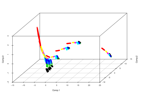
For the purpose of visualizing the data set only, we perform a Principal Components Analysis (PCA) on the set of 9691 96-dimensional Gaia spectra. The first three Principal Components describe 78.25%, 20.44% and 1.02% of the data variance respectively (i.e. 99.71% together). In Fig. 9 we plot the data in projection onto the first three PCs. This diagram, plus the fact that the first three PCs explain almost all of the variance in the data, suggest that a good classification should be possible (the data have an intrinsic low dimensionality).

Figure 9: The 9691 simulated Gaia galaxy spectra with z=0 plotted as their projections onto the first three Principal Components. Black, green, blue, light blue, magenta, yellow and red denote galaxies of type E, Sa, Sb, Sbc, Sc, Sd and Im respectively.

Table 4: Galaxy classification with the SVM. The confusion matrix for the training set for galaxies at z=0. Columns indicate the true class, row the predicted ones.

Type	E-S0	Sa	Sb	Sbc	Sc	Sd	Im
E-S0	1799	0	0	0	0	0	0
Sa	0	1366	0	0	0	0	0
Sb	0	0	53	5	0	0	0
Sbc	0	0	0	134	0	0	0
Sc	0	0	0	0	830	0	0
Sd	0	0	0	0	0	347	1
Im	0	0	0	0	0	0	311

Table 5: As Table 5 but for the test set.

Type	E-S0	Sa	Sb	Sbc	Sc	Sd	Im
E-S0	1798	0	0	0	0	0	0
Sa	0	1329	0	0	0	0	0
Sb	0	0	44	0	0	0	0
Sbc	0	0	4	137	0	0	0
Sc	0	0	0	1	797	0	0
Sd	0	0	0	0	0	394	6
Im	0	0	0	0	0	3	324

The results of training and testing the SVM classifier on the full 96-pixel spectra are shown in Tables 5 and 5. We see that there are very few misclassifications: only 6 and 14 in the training and testing set corresponding to an error of 0.12% and 0.29% respectively. While these results are very promising, it must be recalled that the way the library has been constructed avoids class overlap in the SDSS g$-$r, r$-$i colour space, which surely eases separation in the 96-dimensional BP/RP colour space.

5.1.2 Regression of astrophysical parameters

In addition to simulating an output spectrum, PÉGASE.2 also derives 18 output astrophysical parameters for each galaxy. Of course, by construction we know that our synthetic spectra are uniquely defined by five parameters (p1, p2, infall timescale, age of the galactic winds and the Hubble type), so there can only be five equivalent independent parameters amongst these 18. Nonetheless, it would be useful to predict them directly. Here we build SVM regression models to separately predict the nine most significant ones (listed in Table 6). For each model we train on a randomly selected set of 4846 spectra and evaluate performance on the remaining 4845. In Fig. 10 we present the true and the SVM-predicted values of each parameter on the test set. Table 6 summarizes this by giving the mean of the difference between the true and predicted values for each parameter (which measures the systematic error) as well as the RMS residual (which measures the total scatter). The plots and table indicate that we can predict the parameters to good accuracy and precision, i.e. the systematics are very small and the RMS error is a small fraction of the typical values.

Figure 10: Galaxy parameter estimation performance. For each of the nine APs we plot the predicted vs. true AP values for the test set. The red line indicates the line of perfect estimation. The summary errors are given in Table 6.

Table 6: Summary of the performance of the SVM regression models for predicting the nine APs listed. The sample is for zero redshift but for interstellar extinction ($A_{v}$) varying from 0 to 10 mag. The second and third columns list the mean and RMS errors respectively. The final column gives the number of support vectors in the SVM model.

Astrophysical Parameter	mean(real-predicted)/mean(real)	sd(real-predicted)/mean(real)	SVs
mass to light ratio (M/L)	-1.03e-2	3.78e-2	97
normalized star formation rate (SFR)	-3.35e-3	3.97e-2	2285
metallicity of interstellar medium (Mim)	-2.85e-3	8.77e-2	345
metallicity of stars averaged on mass (Msm)	-3.64e-4	2.17e-2	3544
normalized mass of gas (Mgas)	4.52e-3	4.29e-2	190
normalized mass in stars (Ms)	3.22e-4	5.48e-2	1639
mean age of stars averaged on bolometric luminosity (Al)	1.45e-3	3.22e-2	3566
normalized SNIa rate (SNIa)	9.69e-4	3.43e-2	376
normalized SNII rate (SNII)	-6.04e-4	3.81e-2	2247

5.2 Galaxies with redshift

5.2.1 Regression of redshift and classification of morphological type

We now enlarge the subset of the library we used in the previous tests by adding the same galaxies at four nonzero values of redshift, specifically 0.05, 0.1, 0.15, 0.2. The library for z=0 includes 9691 galaxies as described above. For each nonzero redshift there are 9757 giving a total sample of 48 719 galaxies. (Recall that this includes each galaxy simulated at 11 regular values of $A_{v}$.) We now build another morphological type classification model as done in section 5.1.1, now with 6719 galaxies in the training set and 42 000 galaxies for testing set.

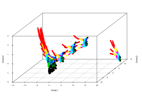
We again applied a PCA to the data. This time the first three Principal Components describe 76.01%, 21.63% and 1.02% of the data variance respectively (i.e. 98.6% together), very similar to before. The corresponding PCA-project plot is Fig. 11. Comparing to Fig. 9 we can see how the redshift spreads out the previous loci of types. The performance of the SVM classifier is summarized in Tables 8 and 8. The performance is good considering the added complexity introduced by the redshift variations (and the corresponding increase in the sample size). The misclassification errors are 0.13% and 0.98% corresponding to 9 and 411 galaxies for the training and the testing data respectively.

Figure 11: The 48 719 simulated Gaia galaxy spectra with nonzero redshift plotted as their projections onto the first three Principal Components. Black, green, blue, light blue, magenta, yellow and red denote galaxies of type E, Sa, Sb, Sbc, Sc, Sd and Im respectively.

Table 7: Galaxy classification with the SVM. The confusion matrix for the training set for galaxies at z=0.0, 0.05, 0.1, 0.15, 0.2. Columns indicate the true class, row the predicted ones.

Type	E-S0	Sa	Sb	Sbc	Sc	Sd	Im
E-S0	2512	0	0	0	0	0	0
Sa	0	1828	0	0	0	0	0
Sb	0	0	74	2	0	0	0
Sbc	0	0	1	183	1	0	0
Sc	0	0	0	0	1115	0	0
Sd	0	0	0	0	0	536	4
Im	0	0	0	0	0	1	462

Table 8: As Table 8 but for the test set.

Type	E-S0	Sa	Sb	Sbc	Sc	Sd	Im
E-S0	15473	0	0	0	0	0	0
Sa	0	11647	0	0	0	0	0
Sb	17	0	344	113	0	0	0
Sbc	0	0	83	1084	23	0	0
Sc	0	0	8	39	6971	7	0
Sd	0	0	0	0	1	3149	50
Im	0	0	0	0	0	70	2921

In practice we may want to first reduce spectra to the rest frame, for which we require an estimate of the redshift. Therefore, we also set up a SVM regression model to predict redshift, using the same training and test sets. The predicted values of redshift for each of the five true redshift values are presented in Fig. 12. We do not expect very good performance here, because the SVM is having to learn the effect of redshift based on just five different values.

Figure 12: Distribution of predicted values of redshift shows separately for the five true values of redshift (z=0, 0.05, 0.1, 0.15 and 0.2)

6 Discussion and conclusion

We have used the PÉGASE.2 galaxy evolution model and the observational data from SDSS to create an extended grid of synthetic galaxy spectra. Using these we have identified the relevant astrophysical parameters and their relevant ranges which provide a realistic galaxy spectra of known morphological type. This was done specifically by comparing the colours of our library spectra with those synthesized from SDSS spectra. We found small deviations between the two colour loci for redder galaxies – where the ellipticals are found – which might be due to the fact that SDSS spectra are obtained in a small aperture (fibre diameter) while PÉGASE spectra are representative of the whole galaxy. We also see that the observed sample has a considerably larger spread in the colour–colour diagram than the library spectra, which probably has observational reasons (photometric errors) as well as theoretical ones (insufficient cosmic variance in the galaxy models). That is, it may partially reflect the complicated nature of galaxy formation and evolution, although the overall agreement between the two is good.

To achieve a better agreement between the observational and synthesized libraries we will further investigate the influence of the various PÉGASE.2 parameters, especially those that were kept constant for this release of the library. On the other hand, due to the narrow redshift range ($z<0.2$) explored here, evolution factors are minimized. At higher redshifts, synthetic spectra will be computed by simultaneously applying cosmological k-corrections and evolution e-corrections to z=0 templates.

Among the existing libraries of observed spectra, the most complete and homogeneous is the SDSS, since it covers a significant part of the whole sky and it goes fainter than the expected detection limit of Gaia. We therefore aim to produce a suitable set of synthetic spectra covering as much as possible of the SDSS colour range and we plan further comparisons in our future work.

Adding phenomena such as the galaxy mergers is a challenging hypothesis, but we believe that at the low redshifts Gaia will observe, this is not such an important or frequent mechanism of galaxy evolution. On the other hand, starburst galaxies are more frequent at small redshifts and we intend to enrich our library with this type of galaxy.

First results of SVM for classification and parametrization of the library are quite promising. In particular, the first indications are that Gaia will be able to produce a wealth of information for a large statistical sample of galaxies. After constructing a more complete library of spectra we will be able to perform more tests and construct a classifier able to treat more realistic and complete simulations of galaxy spectra.

7 Acknowledgments

The authors (the Greek team) would like to thank the Greek General Secretariat of Research and Technology (GSRT) for financial support.

P. Tsalmantza would also like to thank the Max-Planck-Institut für Astronomie (MPIA) and Institut d’Astrophysique de Paris (IAP) for their support and hospitality.

Funding for the Sloan Digital Sky Survey (SDSS) has been provided by the Alfred P. Sloan Foundation, the Participating Institutions, the National Aeronautics and Space Administration, the National Science Foundation, the U.S. Department of Energy, the Japanese Monbukagakusho, and the Max Planck Society. The SDSS Web site is http://www.sdss.org/.

The SDSS is managed by the Astrophysical Research Consortium (ARC) for the Participating Institutions. The Participating Institutions are The University of Chicago, Fermilab, the Institute for Advanced Study, the Japan Participation Group, The Johns Hopkins University, the Korean Scientist Group, Los Alamos National Laboratory, the Max-Planck-Institute for Astronomy (MPIA), the Max-Planck-Institute for Astrophysics (MPA), New Mexico State University, University of Pittsburgh, University of Portsmouth, Princeton University, the United States Naval Observatory, and the University of Washington.

Appendix A Support Vector Machines

Support Vector Machines (SVMs) (Vapnik 1995) are supervised machine learning methods for data classification. In their basic form they achieve a linear classification between two classes by defining an optimal hyperplane which separates members of the two classes. If the classes are separable then there generally exists an infinite number of hyperplanes which achieve this. The SVM optimal plane is defined as that plane which maximises the margin between the opposing class members nearest to the boundary. That is, unlike many other classifiers which use all of the data to define the boundary, SVMs take the (arguably more reasonable) approach of using just those points nearest to the boundary. It has been demonstrated that this gives rise to a more robust and more accurate classifier under general conditions.

In most non-trivial problems, however, the classes are not linearly separable. In these cases, just those points which lie on the wrong side of the hyperplane – the so-called support vectors – enter into the total classification error. By minimizing this error – which also measures the distance of the support vectors from the plane – we define the optimal separating plane, i.e. with the fewest misclassifications (and preferentially of those which lie closer to the plane).

In the general case, the classes are not even marginally linearly separable (consider the XOR problem) so a linear classifier, no matter how optimal, is useless. SVMs address this issue by using kernels to project the data into a higher dimensional space. For example, with a polynomial kernel we take square, cubic etc. combinations of the original data to form additional dimensions and then apply the (linear) SVM classifier in this higher dimensional space. With many other kernels, however, this projection is only carried out implicitly. This approach can be thought of as nonlinearity by preprocessing, with the kernel overcoming the well known “curse of dimensionality”. In the present work we use the radial basis kernel

$$K(x_{i}-x_{j})=exp(-\gamma||x_{i}-x_{j}||^{2})$$ (1)

where $x_{i}$ and $x_{j}$ are two input vectors (e.g. spectra). The classification of a new vector $x_{i}$ is then given by a function

$$f(x_{j})=\sum_{i}^{i=N}y_{i}\alpha_{i}K(x_{i}-x_{j})$$ (2)

where $y_{i}\in(-1,1)$ denotes the two classes, and a classification is made by applying a threshold, e.g. $f(x_{j})>0.0\Rightarrow$ class 1. The ${\alpha_{i}}$ are the parameters of the model which are determined by the model training ($i$ counts over the $N$ support vectors). SVMs have a very important property, namely that the error function is strictly convex, so it has a unique global solution which can be found in polynomial time with standard optimizers (it is a linearly constrained quadratic programming problem).

This is in marked contrast to neural networks, for example, in which the optimizers converge on a local minimum and we can only be guaranteed to find the global minimum via an exhaustive search. Furthermore, with a sigmoidal kernel SVMs are equivalent to neural networks but with the additional advantage that the SVM automatically determines the neural network architecture (number weights).

The SVM model incorporates regularization via the specification of a hyperparameter, $C$, which defines the width of a margin around the separating hyperplane. The wider this margin (larger $C$), the more data vectors which fall into it. These are all considered support vectors and so all enter the error equation. Thus with a larger $C$ there is a higher penalty attached to errors, i.e. less regularization.

The other hyperparameter in the model is $\gamma$ (equation 1). Both $\gamma$ and $C$ must be determined by the user. Prior information may help, but in practice one carries out a rigorous search over a two-dimensional grid to “tune” the SVM. We did this using 4-fold cross validation, iterating over grids of increasing density.

SVMs can also be used for regression. Instead of a hyperplane and a margin about it, regression SVMs fit a line with a tube of radius $\epsilon$ encompassing it. Data vectors which are less than a distance $\epsilon$ from the line are considered to be correctly fit, that is, the support vectors are only those points outside of the tube. Thus the $\epsilon$ hyperparameter controls the degree of regularization. The specific error function we use is the mean squared error on the predictions, with the regularization again being introduced via the constraints in the optimization (with Lagrangian multipliers). All of the kernel and optimization machinery applies equally to these models, so that nonlinear regression can also be achieved.

References

- Armand & Milliard (1994) Armand, C. & Milliard, B. 1994, A&A, 282, 1
- Bennett & Campbell (2000) Bennett, K. P. & Campbell, C. 2000, SIGKDD Explor. Newsl., 2, 1
- Brown (2006) Brown, A. G. A. 2006, Gaia Technical Report GAIA-C8-SP-LEI-AB-006-1
- Buat et al. (1999) Buat, V., Donas, J., Milliard, B., & Xu, C. 1999, A&A, 352, 371
- Burges (1998) Burges, C. J. C. 1998, Data Mining and Knowledge Discovery, 2, 121
- Chang & Lin (2001) Chang, C.-C. & Lin, C.-J. 2001, LIBSVM: a library for support vector machines, software available at http://www.csie.ntu.edu.tw/ cjlin/libsvm
- Fioc (1997) Fioc, M. 1997, PhD thesis, Université Paris XI, http://www.iap.fr/users/fioc.html
- Fioc (1999) Fioc, M. 1999, in Astronomical Society of the Pacific Conference Series, Vol. 192, Spectrophotometric Dating of Stars and Galaxies, ed. I. Hubeny, S. Heap, & R. Cornett, 299–+
- Fioc & Rocca-Volmerange (1997) Fioc, M. & Rocca-Volmerange, B. 1997, A&A, 326, 950
- Fioc & Rocca-Volmerange (1999a) Fioc, M. & Rocca-Volmerange, B. 1999a, A&A, 351, 869
- Fioc & Rocca-Volmerange (1999b) Fioc, M. & Rocca-Volmerange, B. 1999b, A&A, 344, 393
- Fioc & Rocca-Volmerange (1999c) Fioc, M. & Rocca-Volmerange, B. 1999c, arXiv:astro-ph/9912179
- Fukugita et al. (1996) Fukugita, M., Ichikawa, T., Gunn, J. E., et al. 1996, AJ, 111, 1748
- Groenewegen & de Jong (1993) Groenewegen, M. A. T. & de Jong, T. 1993, A&A, 267, 410
- Le Borgne & Rocca-Volmerange (2002) Le Borgne, D. & Rocca-Volmerange, B. 2002, A&A, 386, 446
- Le Borgne et al. (2004) Le Borgne, D., Rocca-Volmerange, B., Prugniel, P., et al. 2004, A&A, 425, 881
- Rana & Basu (1992) Rana, N. C. & Basu, S. 1992, A&A, 265, 499
- Rocca-Volmerange et al. (2007) Rocca-Volmerange, B., de Lapparent, V., Seymour, N., & Fioc, M. 2007, arXiv:0705.2031
- Rocca-Volmerange et al. (2004) Rocca-Volmerange, B., Le Borgne, D., De Breuck, C., Fioc, M., & Moy, E. 2004, A&A, 415, 931
- Vapnik (1995) Vapnik, V. N. 1995, The nature of statistical learning theory (Springer)
- Williams et al. (1996) Williams, R. E., Blacker, B., Dickinson, M., et al. 1996, AJ, 112, 1335
- Woosley & Weaver (1995) Woosley, S. E. & Weaver, T. A. 1995, ApJS, 101, 181