A model for the time uncertainty measurements in the Auger surface detector array

Abstract

The precise determination of the arrival direction of cosmic rays is a fundamental prerequisite for the search for sources or the study of their anisotropies on the sky. One of the most important aspects to achieve an optimal measurement of these directions is to properly take into account the measurement uncertainties in the estimation procedure. In this article we present a model for the uncertainties associated with the time measurements in the Auger surface detector array. We show that this model represents well the measurement uncertainties and therefore provides the basis for an optimal determination of the arrival direction. With this model and a description of the shower front geometry it is possible to estimate, on an event by event basis, the uncertainty associated with the determination of the arrival directions of the cosmic rays.

¹ Centro Brasileiro de Pesquisas Físicas, Rua Dr. Xavier Sigaud 150, Rio de Janeiro, 22290-10, Brazil,
² Laboratoire de Physique Nucléaire et des Hautes Énergies, T33 RdC, 4 place Jussieu, 75252 Paris Cedex 05, France

1 Introduction

The nature and origin of ultra high energy cosmic rays (UHECR) is a continuing puzzle of modern astrophysics [1]. Essential to the study of their origin is the measurement of their arrival directions with a careful evaluation of their measurements uncertainties.

The Pierre Auger Observatory [2] is designed to measure the flux, arrival direction distribution, and composition of the UHECR. In order to have full sky coverage, it will have two components, one in each Hemisphere. The Southern site of the Observatory is in its last stages of construction in Malargüe, Argentina, and has been acquiring data since 2004. When completed, it will be composed of 1,600 water Cherenkov detectors (WCD) spread over 3,000 km² with the atmosphere above viewed by 24 fluorescence telescopes placed in 4 buildings.

Each WCD consists of a rotomolded polyethylene tank with an area of 10 m² and 1.55 m high, enclosing a Tyvek^® liner filled with 12,000 l of high purity water. The Cherenkov light is detected by three large 9” photomultipliers (PMTs) viewing the water tank from the top. Each detector is an autonomous unit. The signals from the PMTs are processed by the local electronics. The power of the whole system is provided by two batteries connected to two solar panels. The time synchronization is done by commercial GPS receivers. There is also a communication system between each detector and the Central Station of the Observatory.

The UHECRs are detected through the particle cascade they produce in the atmosphere. With the Auger surface detector (SD) we determine their arrival direction from a fit to the particle arrival times on the ground.

During the development in the atmosphere, the air shower increases in size up to a maximum. The bulk of the particles reaching the ground are grouped in a thick (hundreds of nano-seconds to a few micro-seconds, e.g. 100 m to 1000 m) nearly spherical pancake. The thickness depends on the distance to the shower axis, while the radius of curvature of the sphere that can be used to describe the shower front approximately depends on the altitude of the shower maximum.

The precision in the cosmic ray arrival direction achieved from the SD reconstruction depends on the clock precision of the detector and on the fluctuations in the first particle arrival time at ground. These fluctuations increase with the shower thickness and decrease with the particle density. Therefore, the shower front time will be measured with less precision for a detector located further away from the core, where particle densities are small and the shower thickness is large, than for the same detector closer to the core of the same shower.

To estimate the primary direction of the primary cosmic ray with the maximum precision, one must, among other things, adequately model the measurement uncertainties of each individual tank participating in the event. These measurement uncertainties depends on the shower properties at each tank location. With an adequate model for the individual measurements, one is able to weight the contribution in the determination of the arrival direction correctly.

The model of the shower front used in the minimization procedure, be it spherical, parabolic, or even planar also influences the uncertainty in the arrival direction determination, but not as much as the time measurement precision. We will show in section 5 that a parabolic model for the shower front adequately describes the data.

In section 2 we describe a model for the shower front particle distribution from which we derive the uncertainty in the time measurement at each tank. In section 3 we implement this model for the Auger WCDs. In section 4 we compare it to measurements obtained using two pairs of adjacent detector stations located in the Auger surface array. Finally, in section 5 we further validate our model by studying the $\chi^{2}$ probability distribution of the geometrical reconstruction of Auger events.

2 A model for the measurement uncertainties

As an estimator for the shower front arrival time ($T_{s}$) at each detector location on the ground it is customary to use the time of the first particle entering the tank. As discussed in the introduction, assuming one has a reasonable description of the shower front geometry, it is the estimation accuracy on $T_{s}$ at each tank that will determine the overall precision with which the Auger SD can reconstruct the primary cosmic ray arrival direction.

At a given point on the ground, we assume that the particle distribution in the shower front can be described as a Poisson process with parameter ${\mathcal{\tau}}$ starting at time $t_{0}$. Of course, both $\mathcal{\tau}$ and $t_{0}$ are functions of the shower characteristics at the considered ground location. In reality, the particle distribution in the shower front is not a uniform Poisson process. At the beginning of the front the particle arrival frequency is larger than towards the end. It is however sufficient to assume that the frequency is constant over some interval large enough to have a good fraction of the total number of particles reaching the ground but less than the total thickness of the shower front at that location.

The first particle arrival time as recorded by the detector clock is then given by:

$$T_{s}=t_{0}+T_{1}$$ (1)

where $T_{1}$ follows an exponential distribution function with decay parameter ${\mathcal{\tau}}$.

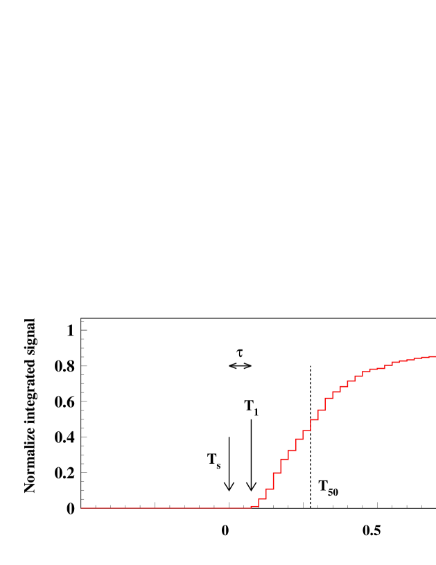
Note that, by construction $T_{s}$ (our shower front arrival time estimator) is always larger than the true (unknown) shower front time $t_{0}$. $T_{s}$ is a biased estimator of $t_{0}$ with a bias given by the expectation of $T_{1}$, $E[T_{1}]=\mathcal{\tau}$. If $\mathcal{\tau}$ is known it would be interesting to construct a new shower front estimator as $T^{\prime}_{s}=T_{s}-{\mathcal{\tau}}$. However, ${\mathcal{\tau}}$ can only be estimated from the shower parameters measured at the ground and is therefore subject to fluctuations. The new estimator $T^{\prime}_{s}$ has therefore slightly larger fluctuations than $T_{s}$ . For an schematic view of our notation see figure 1.

The variance of $T_{s}$ ($V[T_{s}]$) is given by the sum of the detector clock precision ($b^{2}$) and of the variance of the random variable $T_{1}$, $V[T_{1}]=\mathcal{\tau}^{2}$. In practice $\mathcal{\tau}$ is unknown and must be estimated from the data itself. We reverted to use (see section 3) as an estimator of $\mathcal{\tau}$ the ratio of the time of arrival of the $k$-th particle ($T_{k}$) to $k$: $\hat{\tau}=T_{k}/k$. The variance of $T_{s}$ then becomes:

$$V[T_{s}]=\left(\frac{T_{k}}{k}\right)^{2}~{}\frac{k-1}{k+1}+b^{2},$$ (2)

where $b^{2}$ represents the GPS uncertainty and the resolution of the flash analog-to-digital converters (FADCs) of the tanks.

3 Model implementation

To estimate equation 2 for each tank participating in the event we want to reconstruct, we must define ${\mathcal{T}_{k}}$ and $k$ from the data measured at the tank. For $k$ we choose to use the total number of particles entering the tank ($n$ in the following).

The shower signal is recorded in the Auger WCD by the FADCs, which give the signal values in bins of 25 ns as a function of time. From these FADC traces one can build several time parameters such as the time it takes to reach 50% of the total integrated signal in the trace: $T_{50}$ (see figure 1). Following our remark in section 2, we decided to use $2T_{50}$ for $T_{n}$ rather than $T_{100}$ to account for the fact that the Poisson process is not uniform over the whole shower front.

To calculate the total number of particles, $n$, we assume that all particles hit the detector with the same direction as the shower axis, and that the muons (which arrive first) are the ones that contribute most to the time measurements [3]. Then, we obtain $n$ as the ratio between the total integrated signal in the FADC traces in units of vertical equivalent muons [4] (the signal deposited by a central and vertical downgoing muon in a tank), divided by the average muon track length $TL(\theta)$ of a shower with zenith angle $\theta$, normalize to the vertical height ($h$):

$$n=\frac{S_{VEM}}{TL(\theta)/h}.$$ (3)

The average track length $TL(\theta)$ can be computed as the ratio of the detector volume ($V$) and the area ($A$) subtended by the arriving particles at zenith angle $\theta$. For the Auger cylindrical tanks, it is given by:

$$TL(\theta)=\frac{V}{A}=\frac{\pi rh}{\pi r\cos(\theta)+2h\sin(\theta)},$$ (4)

where $r$ = 1.8 m is the detector radius, and $h$ = 1.2 m is the water height in the detector.

We further introduce a scale parameter $a$ to account for the various approximations made to build $V[T_{s}]$ and finally define it as:

$$V[T_{s}]=a^{2}~{}\left(\frac{2~{}T_{50}}{n}\right)^{2}~{}\frac{n-1}{n+1}+b^{2}.$$ (5)

Parameters $a$ and $b$ can be determined from the data of the two pairs of adjacent stations available in the Auger array (see section 4.1). We expect, however, $a$ to be close to unity and to $b$ be given by our GPS system resolution [5] (10 ns) and the resolution of our FADC traces (25/$\sqrt{12}$ ns), giving $b\simeq 12$ ns.

4 Comparison with data

4.1 Fitting the doublet data

Two pairs of adjacent surface detector stations separated by 11 m (“doublets”) have been installed in the field of the Auger Observatory. These pairs enable comparison of timing and signal accuracy measurements.

To adjust the constants $a$ and $b$ we used all the T4 [6] events from April 2004 to the end of December 2006, with at least one doublet information available. We defined the time difference $\Delta T=dT_{1}-dT_{2}$ where $dT_{1}$ ($dT_{2}$) is the time residual of the first (second) twin tank to the fitted shower front. Note that using the residual difference assures that $\Delta T$ does not depend on the global shower front shape, since the twin tanks are only 11 m apart.

The knowledge of $\Delta T$ only requires the knowledge of $\theta$ and $\phi$ with moderate precision (a few degrees is enough). We further required $\mid\Delta T\mid$ to be smaller than 200 ns to avoid the tails of the distribution and also a good overall reconstruction. With these cuts we had 2037 events to fit our two parameters $a$ and $b$.

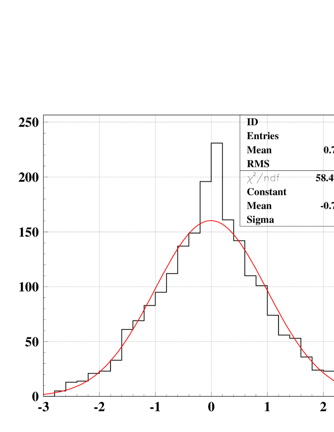
Since the distribution of $\Delta T/\sqrt{V[\Delta T]}$ is close to a Gaussian (see figure 2), we fit the parameters by maximizing the following likelihood function (L):

$$\emph{L}=\prod_{k=1}^{N}\frac{1}{\sqrt{2\pi V[\Delta T_{k}]~{}}}~{}~{}e^{-\frac{\Delta T^{2}_{k}}{2~{}V[\Delta T_{k}]}}$$ (6)

where $N$ is the total number of events and $V[\Delta T_{k}]=V[T_{1,k}]+V[T_{2,k}]$ is calculated from the variance of $T_{s}$ for each member of the doublet and for each event $k$ using equation 5. Maximizing L is equivalent to minimizing $\emph{Z}=-2\ln(\emph{L})$, which was done using the Minuit package. We obtained:

$$\begin{array}[]{ccrcl}a^{2}&=&0.97\pm 0.04,{}{}{}{}{}\\ b^{2}&=&\left(132\pm 11\right)~{}\mbox{\rm ns}^{2}.\end{array}$$

These results are in remarkable agreement with the values expected from the model definition: $a^{2}~{}=~{}1$ and $b^{2}~{}=~{}144~{}ns^{2}$.

As mentioned earlier, we expect the distribution of the variable $\Delta T$ to be essentially insensitive to the details of the geometrical reconstruction used to derive it. This is because the two tanks in a doublet are very close together and $\Delta T$ can be computed with moderate precision based on the shower angles (a few degrees) and regardless of the general structure of the shower front. We verified that indeed the parameters $a$ and $b$ did not depend on the nature and quality of the initial geometrical fit used when analyzing the doublet data. We used, for example, values for $a$ and $b$ different from 1 and 12 during the shower geometrical fit, and also replaced our time variance model by a constant, we always obtained the same final parameters values (within the uncertainties). This shows that using the doublets and the estimator $\Delta T$ we are really independent of the details of the geometrical reconstruction used to determined the model parameters.

4.2 Model quality

The value of L at the minimum (10.9 per degree of freedom) is quite meaningless (unlike a $\chi^{2}$ value), therefore we need to evaluate the quality of the fit using alternative tests.

We computed the quality $\chi^{2}=\sum_{k=1}^{ndof}\frac{\Delta T_{k}^{2}}{V[\Delta T_{k}]}$, which should be close to the number of degrees of freedom if $V[\Delta T_{k}]$ properly models the variance of $\Delta T$. We obtained at the minimum $\chi^{2}/ndof=$ 1.00097.

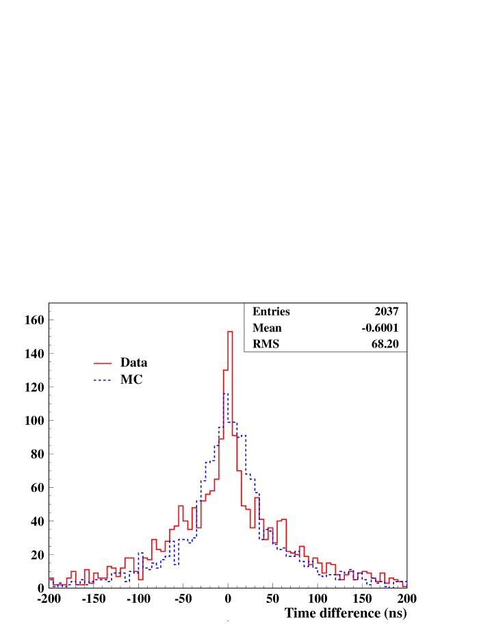
We also generated a Monte Carlo sample based on the doublet data. For each event with a doublet we used the values of $T_{50}$ and signal ($S$) of the doublet members and draw a new time value according to our shower front model, plus a 25 ns uniform distribution corresponding to our FADC bin size and a Gaussian distribution with $\sigma=10$ ns corresponding to the GPS clock accuracy. We then calculated $\Delta T$ as the difference of these two times and reproduced our analysis on this MC sample.

From the minimization of Z, we obtain on the MC sample:

$$\begin{array}[]{ccr}a^{2}&=&0.74\pm 0.05,{}{}{}{}{}\\ b^{2}&=&\left(215\pm 28\right)~{}\mbox{\text{n}s}^{2}.\end{array}$$

with a value of $\emph{Z}=10.6$ and $\chi^{2}=1.0011$ at the minimum, which are similar to what we obtained with the real data and also corresponds to the injected parameters.

In addition, in figure 3 we plot for comparison $\Delta T$ distributions for the doublet data (red-solid) and for the Monte Carlo (blue-dashed). As can be seen, the agreement is good.

5 Validation

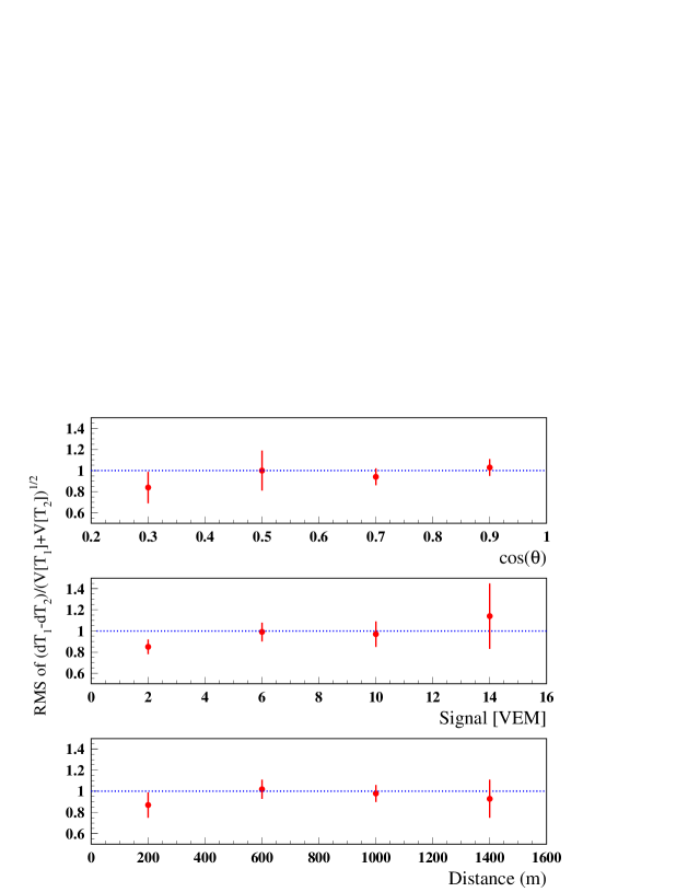
If the time variance model describes correctly the measurement uncertainties, the distribution of $\Delta T/\sqrt{V[\Delta T]}$, where $V[\Delta T]~{}=~{}V[T_{1}^{(1)}]~{}+~{}V[T_{1}^{(2)}]$, should have unit variance.

We show on figure 4 the RMS of the distributions of $\Delta T/\sqrt{V[\Delta T]}$ for various bins in $\cos(\theta)$ (top), in signal (middle), and in distance to core (bottom). In the three cases, it is almost constant and close to unity, which shows that our model for the time uncertainty is in good agreement with the experimental data. It is important to remark that our model does not depend directly on the distance of the tank to the shower core. Therefore, the results obtained in this case can be regarded as an additional proof of validity.

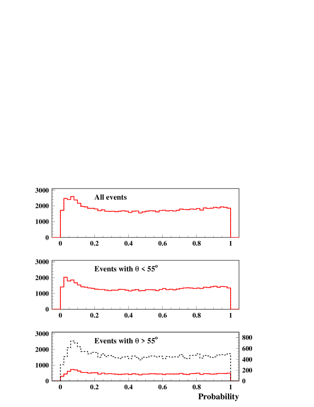
We also studied the distribution of the $\chi^{2}$ probability of the T5 events [6] with 4 or more stations. In figure 5 we show this distribution for all events (top), for events with zenith angle smaller than 55^∘ (middle) and events with zenith angle larger than 55^∘ (bottom). For the three cases, the distributions are almost flat as it should be in the ideal case. It is important that the flatness is observed both for large and small zenith angles separately, which means that the model for the time uncertainty works well for all angles without compensating one set from the other. The flatness of these distributions indicates that our model properly reproduces the experimental uncertainty. It also indicates that the shower front model used in our fit (parabolic front with adjusted radius) is adequate.

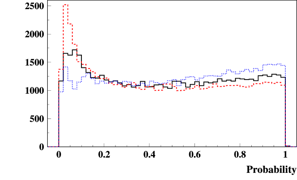
Finally, to illustrate the sensitivity of the $\chi^{2}$ probability distribution to the value of the variance used in the fit, we plotted in figure 6 the distribution obtained when one artificially varies the overall variance (e.g. $\chi^{2}$) normalization. In black (solid), the original curve, in red (dashed) for a variance reduced by 20% (individual $\chi^{2}$ mutliplied by 1.2), in blue (dotted) increased by 20% (individual $\chi^{2}$ multiplied by 0.8). This 20% in $\chi^{2}$ is equivalent to a 10% change in $\sigma$. We therefore conclude that we properly reproduce the measurement uncertainties within 10% level.

6 Conclusions

We developed a model to describe the measurement uncertainties of the arrival direction of the shower front for an air-shower surface detector array. This model is used for the Auger WCD and is based on the shower zenith angle, integrated signal and rise time measured in the tanks. Absolute predictions of our model parameters for the time uncertainty measurements are consistent with the ones obtained from analysis of adjacent tank data.

We performed numerous tests to validate both our estimation methods and our modeled values. All cases indicated a correct procedure and a good agreement with the experimental data.

This model together with the proper description of the front geometry will allow for an optimal determination of the shower arrival direction. Properly taking into account our measurement uncertainties also allows for an event by event determination of the precision on the reconstructed arrival direction.

7 Acknowledgments

This work was supported by the Conselho Nacional de Desenvolvimento Científico e Tecnológico (CNPq), Brazil, and the Centre National de la Recherche Scientifique, Institut National de Physique Nucléare et Physique des Particules (IN2P3/CNRS), France. LEO - International Research Group.

Figure 1: Example of an integrated FADC trace for a detector at  700 m from the shower core position. $T_{s}$ is the shower front arrival time, $T_{1}$ is the arrival time of the first particles, and $T_{50}$ is the time it takes to reach 50% of the total integrated signal in the trace.

Figure 2: Distribution of $\Delta T/\sqrt{(}V[\Delta T])$ where $V[\Delta T]=V[T_{1}]+V[T_{2}]$ with $T_{1}$ ($T_{2}$) calculated using equation 5 for the first (second) twin tank, with $a=1$ and $b=12$ ns.

Figure 3: Comparison of the $\Delta T$ distributions for doublet data (red-solid) and for MC events (blue-dashed).

Figure 4: The RMS of the distribution of $\Delta T/\sqrt{V[\Delta T]}$, as a function of the shower zenith angle (top), the average signal in the doublet detectors (middle), and the distance to the shower core (bottom).

Figure 5: The $\chi^{2}$ probability distribution for all events (top), events with zenith angle smaller than 55^∘ (middle), and events with zenith angle larger than 55^∘ (bottom). In the last figure the distribution is plotted with two different scales, the same than the others (full line) for comparison reasons and a zoom (dashed line) to see the details.

Figure 6: Distribution of the probability of $\chi^{2}$, in black (solid) the original one, in red (dashed) 1.2 $\chi^{2}$ and in blue (dot) 0.8 $\chi^{2}$.

References

- [1] M. Nagano and A. A. Watson, Rev. Mod. Phys. 72 689-732 (2000).
- [2] J. Abraham et al., Pierre Auger Collaboration: 2005, Nucl. Intr. & Meth. A523, 50-95 (2005)
- [3] J. Linsley and L. Scarsi, Phys. Rev. 128, 2384-2392 (1962)
- [4] X. Bertou et al., Nucl. Intr. & Meth. accepted to be published in Nucl. Intr. & Meth. (2006)
- [5] X. Bertou for Pierre Auger Collaboration, 29th ICRC Pune, 7, 1-4 (2005)
- [6] D. Allard et al., Pierre Auger Collaboration, 29th ICRC Pune, 7, 287-290 (2005)