DESY-07-059

SFB/CPP-07-17

MIT-CTP 3838

Non-perturbative renormalization of the chromo-magnetic operator in Heavy Quark Effective Theory and the B – B mass splitting.

Damiano Guazzinia, Harvey Meyerb and Rainer Sommera
a DESY, Platanenallee 6, 15738 Zeuthen, Germany b Center for Theoretical Physics, Massachusetts Institute of Technology

Cambridge, MA 02139, U.S.A.
Abstract

We carry out the non-perturbative renormalization of the chromo-magnetic operator in Heavy Quark Effective Theory. At order 1/m1𝑚1/m of the expansion, the operator is responsible for the mass splitting between the pseudoscalar and vector B𝐵B mesons. We obtain its two-loop anomalous dimension in a Schrödinger functional scheme by successive one-loop conversions to the lattice MS scheme and the MS¯¯MS\overline{\rm MS} scheme. We then compute the scale evolution of the operator non-perturbatively in the Nf=0subscript𝑁f0N_{\rm f}=0 theory between μ0.3𝜇0.3\mu\approx 0.3 GeV and μ100𝜇100\mu\approx 100 GeV, where contact is made with perturbation theory. The overall renormalization factor that converts the bare lattice operator to its renormalization group invariant form is given for the Wilson gauge action and two standard discretizations of the heavy-quark action. As an application, we find that this factor brings the previous quenched predictions of the B – B mass splitting closer to the experimental value than found with a perturbative renormalization. The same renormalization factor is applicable to the spin-dependent potentials of Eichten and Feinberg. Key words: Lattice QCD; Heavy quark effective theory; Non-perturbative renormalization; Hadron spectrum PACS: 11.10.Gh; 11.15.Ha; 12.38.Gc; 12.39.Hg; 14.40.Nd; 14.65.Fy


May 2007

1 Introduction

Heavy-light bound states in QCD can be described efficiently by an expansion in the inverse heavy quark mass. Already in the early days of the associated effective field theory, HQET [?,?,?], the mass splitting between vector and pseudo-scalar heavy-light mesons served as a phenomenological argument for the absence of large higher order corrections in the expansion.

Consider QCD with Nfsubscript𝑁fN_{\rm f} light quark flavors and a heavy flavor, the b-quark, Nf=4subscript𝑁f4N_{\rm f}=4 being the case realized in Nature. The splitting

Δm2mB2mB2Δsuperscript𝑚2superscriptsubscript𝑚superscriptB2superscriptsubscript𝑚B2\displaystyle\Delta m^{2}\equiv m_{\mathrm{B^{*}}}^{2}-m_{\mathrm{B}}^{2} (1.1)

then has an asymptotic behavior for large quark mass mbsubscript𝑚bm_{{\rm b}} which is characterized by one renormalization group invariant (RGI) observable,

4λ2RGI4superscriptsubscript𝜆2RGI\displaystyle 4\lambda_{2}^{\rm RGI} =\displaystyle= limmb{[ 2b0g¯2(mb)]γ0/2b0Δm2},subscriptsubscript𝑚bsuperscriptdelimited-[]2subscript𝑏0superscript¯𝑔2subscript𝑚bsubscript𝛾02subscript𝑏0Δsuperscript𝑚2\displaystyle\lim_{m_{{\rm b}}\to\infty}\left\{\left[\,2b_{0}\bar{g}^{2}(m_{{\rm b}})\,\right]^{-\gamma_{0}/2b_{0}}\Delta m^{2}\right\}\,,
(γ0=3/(8π2),b0=(1123Nf)/(16π2))formulae-sequencesubscript𝛾038superscript𝜋2subscript𝑏01123subscript𝑁f16superscript𝜋2\displaystyle\big{(}\;\gamma_{0}=3/(8\pi^{2})\,,\;\;b_{0}=(11-\hbox{$2\over 3$}N_{\rm f})/(16\pi^{2})\big{)}

of dimension [mass]2. Since the limit exists, this quantity is uniquely defined in QCD. In the above the definition of mbsubscript𝑚bm_{{\rm b}} is irrelevant as long as it is renormalized at a scale of order mbsubscript𝑚bm_{{\rm b}}.

As a rather non-trivial statement, the effective field theory predicts that λ2RGIsuperscriptsubscript𝜆2RGI\lambda_{2}^{\rm RGI} can unambiguously be computed in that theory, where the b-quark is treated as static. There it is expressed as an expectation value

λ2RGIsuperscriptsubscript𝜆2RGI\displaystyle\lambda_{2}^{\rm RGI} =\displaystyle= 13B|𝒪spinRGI|B/B|B,13quantum-operator-product𝐵superscriptsubscript𝒪spinRGI𝐵inner-product𝐵𝐵\displaystyle\hbox{$1\over 3$}\langle B|{\cal O}_{\mathrm{spin}}^{\rm RGI}|B\rangle\,/\,\langle B|B\rangle\,, (1.3)
𝒪spinRGIsuperscriptsubscript𝒪spinRGI\displaystyle{\cal O}_{\mathrm{spin}}^{\rm RGI} =\displaystyle= limμ[ 2b0g¯2(μ)]γ0/2b0𝒪spinS(μ),subscript𝜇superscriptdelimited-[]2subscript𝑏0superscript¯𝑔2𝜇subscript𝛾02subscript𝑏0superscriptsubscript𝒪spin𝑆𝜇\displaystyle\lim_{\mu\to\infty}\left[\,2b_{0}\bar{g}^{2}(\mu)\,\right]^{-\gamma_{0}/2b_{0}}{\cal O}_{\mathrm{spin}}^{S}(\mu)\,, (1.4)

of 𝒪spinRGIsuperscriptsubscript𝒪spinRGI{\cal O}_{\mathrm{spin}}^{\rm RGI} in the zero-momentum B-meson state |Bket𝐵|B\rangle. The operator 𝒪spinSsuperscriptsubscript𝒪spin𝑆{\cal O}_{\mathrm{spin}}^{S} is related to the bare local operator

𝒪spin(x)=ψ¯h(x)12iFkl(x)σklψh(x)=ψ¯h(x)𝝈𝐁(x)ψh(x)subscript𝒪spin𝑥subscript¯𝜓h𝑥12𝑖subscript𝐹𝑘𝑙𝑥subscript𝜎𝑘𝑙subscript𝜓h𝑥subscript¯𝜓h𝑥𝝈𝐁𝑥subscript𝜓h𝑥{\cal O}_{\mathrm{spin}}(x)=\overline{\psi}_{\rm h}(x){1\over 2i}F_{kl}(x)\sigma_{kl}\psi_{\rm h}(x)=\overline{\psi}_{\rm h}(x){\boldsymbol{\sigma}}\!\cdot\!{\bf B}(x)\psi_{\rm h}(x) (1.5)

by a multiplicative renormalization depending on the adopted scheme S𝑆S and a renormalization scale μ𝜇\mu – but 𝒪spinRGIsuperscriptsubscript𝒪spinRGI{\cal O}_{\mathrm{spin}}^{\rm RGI} neither depends on a scheme nor on a scale.

The matrix element of the bare operator can be computed non-perturbatively by lattice simulations of HQET [?,?,?]. As stated in these references, a significant source of uncertainty remained in the connection between the bare operator and the RGI one (or one renormalized in the MS¯¯MS{\rm\overline{MS\kern-0.50003pt}\kern 0.50003pt} scheme), which has only been established perturbatively [?,?]. This uncertainty made it impossible to decide whether the splitting is significantly underestimated in the quenched approximation (Nf=0subscript𝑁f0N_{\rm f}=0) or not.

In this paper we develop the non-perturbative renormalization of 𝒪spinsubscript𝒪spin{\cal O}_{\mathrm{spin}}. We follow the general strategy of the ALPHA-collaboration [?,?,?], specialize it to the operator in question and perform an explicit computation in the quenched approximation. In particular we define a suitable scheme using Schrödinger functional (SF) boundary conditions, and compute the 2-loop anomalous dimension in this scheme. We then evaluate the scale dependence of the operator non-perturbatively for Nf=0subscript𝑁f0N_{\rm f}=0, between μ0.3GeV𝜇0.3GeV\mu\approx 0.3\,{\rm GeV} and μ100GeV𝜇100GeV\mu\approx 100\,{\rm GeV}. Using the high energy end of the results and eq. (1.4) supplemented with the 2-loop anomalous dimension, the connection to the RGI operator is realized. Finally the total Z𝑍Z-factor between bare and RGI operator is obtained for the Wilson gauge action and several HQET discretizations. Readers solely interested in the final result for the Z𝑍Z-factor may find it in Sect. 5.1.

For a comparison to the experimental mass splitting at finite mass, it is important to include radiative corrections beyond the 1-loop ones incorporated in eq. (1). We do this in the form

Δm2=2mB+mBMbCspin(Mb/ΛMS¯)λ2RGI+O(1/mb),Δsuperscript𝑚22subscript𝑚superscriptBsubscript𝑚Bsubscript𝑀bsubscript𝐶spinsubscript𝑀bsubscriptΛ¯MSsuperscriptsubscript𝜆2RGIO1subscript𝑚b\Delta m^{2}=2{m_{\mathrm{B^{*}}}+m_{\mathrm{B}}\over M_{{\rm b}}}C_{\rm spin}(M_{{\rm b}}/\Lambda_{{\rm\overline{MS\kern-0.35002pt}\kern 0.35002pt}})\lambda_{2}^{\rm RGI}+{\rm O}(1/m_{\mathrm{b}})\,, (1.6)

written in terms of RGI’s with a function Cspinsubscript𝐶spinC_{\rm spin} known up to corrections O(α2(mb))4%Osuperscript𝛼2subscript𝑚bpercent4{\rm O}(\alpha^{2}(m_{{\rm b}}))\approx 4\,\% and discussed in some detail in Sect. 2. Obviously the perturbative uncertainty can be estimated more reliably and reduced by a higher order continuum perturbative computation in QCD. We note that the final renormalization factor ZspinRGIsuperscriptsubscript𝑍spinRGIZ_{\rm spin}^{\rm RGI} also applies to spin-dependent potentials computed in lattice gauge theory (see Sect. 3).

The reader is not to confuse the present approach with the one of [?,?], where, through a non-perturbative matching between QCD and HQET, also functions such as Cspinsubscript𝐶spinC_{\rm spin} are determined non-perturbatively. While in general the strategy of [?,?] is essential, the more traditional path is viable here because 𝒪spinsubscript𝒪spin{\cal O}_{\mathrm{spin}} does not mix with lower dimensional operators.

Before entering the discussion of the renormalization of 𝒪spinsubscript𝒪spin{\cal O}_{\mathrm{spin}}, we briefly address the question of the precision that can be expected from eq. (1.6). For this purpose we boldly also treat Δmc2=mD2mD2Δsubscriptsuperscript𝑚2csubscriptsuperscript𝑚2superscriptDsubscriptsuperscript𝑚2D\Delta m^{2}_{\rm c}=m^{2}_{\rm D^{*}}-m^{2}_{\rm D} in HQET. So Nf=3subscript𝑁f3N_{\rm f}=3 in all places. With a Nf=3subscript𝑁f3N_{\rm f}=3 QCD-parameter of ΛMS¯(3)=300(100)MeVsuperscriptsubscriptΛ¯MS3300100MeV\Lambda_{{\rm\overline{MS\kern-0.35002pt}\kern 0.35002pt}}^{(3)}=300(100)\,{\rm MeV} and with Mc=1.55GeVsubscript𝑀c1.55GeVM_{{\rm c}}=1.55\,{\rm GeV}, Mb=6.69GeVsubscript𝑀b6.69GeVM_{{\rm b}}=6.69\,{\rm GeV} [?] we find Mc/Mb0.23subscript𝑀csubscript𝑀b0.23M_{{\rm c}}/M_{{\rm b}}\approx 0.23 and Cspin(Mc/ΛMS¯)/Cspin(Mb/ΛMS¯)=0.94subscript𝐶spinsubscript𝑀csubscriptΛ¯MSsubscript𝐶spinsubscript𝑀bsubscriptΛ¯MS0.94C_{\rm spin}(M_{{\rm c}}/\Lambda_{\rm\overline{MS\kern-0.35002pt}\kern 0.35002pt})/C_{\rm spin}(M_{{\rm b}}/\Lambda_{\rm\overline{MS\kern-0.35002pt}\kern 0.35002pt})=0.94 . HQET then relates the splittings as Δmc2/Δm2=1.41(2)Δsubscriptsuperscript𝑚2cΔsuperscript𝑚21.412\Delta m^{2}_{\rm c}/\Delta m^{2}=1.41(2), where the uncertainty is due to the generous error in ΛMS¯(3)superscriptsubscriptΛ¯MS3\Lambda_{{\rm\overline{MS\kern-0.35002pt}\kern 0.35002pt}}^{(3)}. With the quenched input values ΛMS¯=238MeV,Mc=1.65GeV,Mb=6.76GeVformulae-sequencesubscriptΛ¯MS238MeVformulae-sequencesubscript𝑀c1.65GeVsubscript𝑀b6.76GeV\Lambda_{{\rm\overline{MS\kern-0.35002pt}\kern 0.35002pt}}=238\,{\rm MeV},\,M_{{\rm c}}=1.65\,{\rm GeV},\,M_{{\rm b}}=6.76\,{\rm GeV} [?,?,?,?] this ratio changes only slightly, namely to Δmc2/Δm21.44Δsubscriptsuperscript𝑚2cΔsuperscript𝑚21.44\Delta m^{2}_{\rm c}/\Delta m^{2}\approx 1.44. This is to be compared to Δmc2/Δm2=1.14Δsubscriptsuperscript𝑚2cΔsuperscript𝑚21.14\Delta m^{2}_{\rm c}/\Delta m^{2}=1.14 from experiment.

Since the charm mass is only moderately large, such a 25% deviation is not unexpected. Scaling this correction to the B-system, we expect an accuracy of order 5-10% for the HQET prediction of Δm2Δsuperscript𝑚2\Delta m^{2}. Earlier quenched approximation estimates with perturbative renormalization found values for Δm2Δsuperscript𝑚2\Delta m^{2} which were lower than the experimental number by between 50% [?,?] and 20% [?]. Renormalizing the same matrix elements non-perturbatively we will find the difference to experiment significantly reduced in Sect. 6.

2 HQET and λ2RGIsuperscriptsubscript𝜆2RGI\lambda_{2}^{\rm RGI}

2.1 Lattice action

We briefly define the effective theory in a lattice regularization, using the notation of [?,?]. The heavy quark fields are taken to have 4 components with the constraint

P+ψh=ψh,ψ¯hP+=ψ¯hP+=12(1+γ0).formulae-sequencesubscript𝑃subscript𝜓hsubscript𝜓hformulae-sequencesubscript¯𝜓hsubscript𝑃subscript¯𝜓hsubscript𝑃121subscript𝛾0P_{+}\psi_{\rm h}=\psi_{\rm h}\,,\quad\overline{\psi}_{\rm h}P_{+}=\overline{\psi}_{\rm h}\,\quad P_{+}=\hbox{$1\over 2$}(1+\gamma_{0})\,. (2.7)

With the lattice backward derivative

D0Wψh(x)=1a[ψh(x)W(xa0^,0)ψh(xa0^)],superscriptsubscript𝐷0Wsubscript𝜓h𝑥1𝑎delimited-[]subscript𝜓h𝑥superscript𝑊𝑥𝑎^00subscript𝜓h𝑥𝑎^0D_{0}^{\rm W}\psi_{\rm h}(x)={{1}\over{a}}\left[\psi_{\rm h}(x)-W^{\dagger}(x-a\hat{0},0)\psi_{\rm h}(x-a\hat{0})\right]\;, (2.8)

and the mass counterterm δmW𝛿subscript𝑚W\delta m_{\rm W}, the static action (i.e. lowest order HQET) is written as

ShW=a411+aδmWxψ¯h(x)(D0W+δmW)ψh(x).superscriptsubscript𝑆hWsuperscript𝑎411𝑎𝛿subscript𝑚Wsubscript𝑥subscript¯𝜓h𝑥superscriptsubscript𝐷0W𝛿subscript𝑚Wsubscript𝜓h𝑥S_{\rm h}^{\rm W}=a^{4}{{1}\over{1+a\;\delta m_{\rm W}}}\sum_{x}\overline{\psi}_{\rm h}(x)(D_{0}^{\rm W}+\delta m_{\rm W})\psi_{\rm h}(x)\;. (2.9)

Different gauge connections W𝑊W have been found to be very useful to improve the statistical precision in numerical simulations [?,?]. They play a rôle only when we discuss the non-perturbative results. Until then the reader may think of W(x,0)𝑊𝑥0W(x,0) as the standard timelike link. In fact that choice defines the original Eichten-Hill action [?].

2.2 Conversion functions

The operator 𝒪spin(x)subscript𝒪spin𝑥{\cal O}_{\mathrm{spin}}(x) in eq. (1.5) is given in terms of the fields entering eq. (2.9) with the normalization specified there. The lattice version F^μνsubscript^𝐹𝜇𝜈\hat{F}_{\mu\nu} of the gauge field tensor is defined by the clover leaf term, see e.g. [?]. 𝒪spinsubscript𝒪spin{\cal O}_{\mathrm{spin}} appears as a first order correction in 1/mb1subscript𝑚b1/m_{\mathrm{b}} in HQET and induces the spin splitting. Usually, the splitting is written in a form different from eq. (1.6). We want to briefly explain why we choose the latter.

The more common form is

mB2mB2superscriptsubscript𝑚superscriptB2superscriptsubscript𝑚B2\displaystyle m_{\mathrm{B^{*}}}^{2}-m_{\mathrm{B}}^{2} =\displaystyle= 4Cmagmatch(mb)λ2(mb)+O(1/mb)4subscriptsuperscript𝐶matchmagsubscript𝑚bsubscript𝜆2subscript𝑚bO1subscript𝑚b\displaystyle 4\,C^{\rm match}_{\rm mag}(m_{{\rm b}})\,\lambda_{2}(m_{{\rm b}})+{\rm O}(1/m_{\mathrm{b}}) (2.10)
λ2(mb)subscript𝜆2subscript𝑚b\displaystyle\lambda_{2}(m_{{\rm b}}) =\displaystyle= 13B|𝒪spinMS¯(μ=mb)|B13quantum-operator-product𝐵superscriptsubscript𝒪spin¯MS𝜇subscript𝑚b𝐵\displaystyle{1\over 3}\,\langle B|{\cal O}_{\mathrm{spin}}^{\rm\overline{MS\kern-0.35002pt}\kern 0.35002pt}(\mu=m_{{\rm b}})|B\rangle (2.11)

where 𝒪spinMS¯superscriptsubscript𝒪spin¯MS{\cal O}_{\mathrm{spin}}^{\rm\overline{MS\kern-0.35002pt}\kern 0.35002pt} and mbsubscript𝑚bm_{{\rm b}} are renormalized in the MS¯¯MS{\rm\overline{MS\kern-0.50003pt}\kern 0.50003pt} scheme. This is arrived at by starting from the formal expression

mBmBsubscript𝑚superscriptBsubscript𝑚B\displaystyle m_{\mathrm{B^{*}}}-m_{\mathrm{B}} similar-to\displaystyle\sim 231mbB|𝒪spin|B/B|B.231mbquantum-operator-product𝐵subscript𝒪spin𝐵inner-product𝐵𝐵\displaystyle\hbox{$2\over 3$}\hbox{$1\over m_{{\rm b}}$}\langle B|{\cal O}_{\mathrm{spin}}|B\rangle\,/\,\langle B|B\rangle\,. (2.12)

One renormalizes 𝒪spinsubscript𝒪spin{\cal O}_{\mathrm{spin}} in the MS¯¯MS{\rm\overline{MS\kern-0.50003pt}\kern 0.50003pt} scheme, identifies the mass mbsubscript𝑚bm_{{\rm b}} with the (perturbative) pole mass mQ,bsubscript𝑚Qbm_{\rm Q,{\rm b}} and defines the remaining factor as a matching coefficient Cmagmatch(mb)subscriptsuperscript𝐶matchmagsubscript𝑚bC^{\rm match}_{\rm mag}(m_{{\rm b}}). Finally one uses 2mQ,b=mB+mB+O(Λ)2subscript𝑚Qbsubscript𝑚superscriptBsubscript𝑚BOΛ2m_{\rm Q,{\rm b}}=m_{\mathrm{B^{*}}}+m_{\mathrm{B}}+{\rm O}(\Lambda), dropping the O(Λ)OΛ{\rm O}(\Lambda) correction.

The matching coefficient Cmagmatch(mb)=1+C1g¯2(mb)+subscriptsuperscript𝐶matchmagsubscript𝑚b1subscript𝐶1superscript¯𝑔2subscript𝑚bC^{\rm match}_{\rm mag}(m_{{\rm b}})=1+C_{1}\bar{g}^{2}(m_{{\rm b}})+\ldots is independent of the particular matrix element. Since mb4GeVsubscript𝑚b4GeVm_{{\rm b}}\approx 4{\rm GeV} is reasonably large and there is no mixing with lower dimensional operators, Cmagmatchsubscriptsuperscript𝐶matchmagC^{\rm match}_{\rm mag} can be approximated by perturbation theory. It is known including the C1g¯2(mb)subscript𝐶1superscript¯𝑔2subscript𝑚bC_{1}\bar{g}^{2}(m_{{\rm b}}) term [?].

In the above form, the matrix element and the HQET parameter λ2subscript𝜆2\lambda_{2} depend on the arbitrary renormalization scheme (MS¯¯MS{\rm\overline{MS\kern-0.50003pt}\kern 0.50003pt}). Such a spurious dependence is easily removed by introducing RGIs (see e.g. [?] and Sect.III.3.1.of[?]), in particular 𝒪spinRGIsuperscriptsubscript𝒪spinRGI{\cal O}_{\mathrm{spin}}^{\rm RGI}, eq. (1.4). It is related to the bare operator 𝒪spinsubscript𝒪spin{\cal O}_{\mathrm{spin}} in a particular lattice regularization via

𝒪spinRGIsuperscriptsubscript𝒪spinRGI\displaystyle{\cal O}_{\mathrm{spin}}^{\rm RGI} =\displaystyle= ZspinRGI(g0)𝒪spin.superscriptsubscript𝑍spinRGIsubscript𝑔0subscript𝒪spin\displaystyle Z_{\rm spin}^{\rm RGI}(g_{0}){\cal O}_{\mathrm{spin}}\,. (2.13)

We now have

mB2mB2superscriptsubscript𝑚superscriptB2superscriptsubscript𝑚B2\displaystyle m_{\mathrm{B^{*}}}^{2}-m_{\mathrm{B}}^{2} =\displaystyle= 4Cmag(Mb/ΛMS¯)λ2RGI+O(1/mb)4subscript𝐶magsubscript𝑀bsubscriptΛ¯MSsuperscriptsubscript𝜆2RGIO1subscript𝑚b\displaystyle 4C_{\rm mag}(M_{{\rm b}}/\Lambda_{{\rm\overline{MS\kern-0.35002pt}\kern 0.35002pt}})\lambda_{2}^{\rm RGI}+{\rm O}(1/m_{\mathrm{b}})\, (2.14)

with a function Cmag(Mb/ΛMS¯)subscript𝐶magsubscript𝑀bsubscriptΛ¯MSC_{\rm mag}(M_{{\rm b}}/\Lambda_{{\rm\overline{MS\kern-0.35002pt}\kern 0.35002pt}}) written in terms of the RGI mass of the b-quark and the QCD ΛΛ\Lambda-parameter. Using existing perturbative computations [?,?,?,?] it is easily evaluated by integration of the RG equations (see e.g. [?]).
Refer to caption
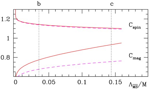
Figure 1: Conversion functions for Nf=0subscript𝑁f0N_{\rm f}=0. Dashed lines for 1-loop anomalous dimension and continuous line for 2-loop γ𝛾\gamma. In the latter case the parametric uncertainty is O(α2(mb))Osuperscript𝛼2subscript𝑚b{\rm O}(\alpha^{2}(m_{{\rm b}})). The abscissas of the c quark and the b quark are marked by vertical dots.

The comparison of the successive perturbative approximations for Cmagsubscript𝐶magC_{\rm mag} in Fig. 1 indicates a relatively large perturbative error even at the 2-loop level (for the anomalous dimension γ𝛾\gamma). At a scale of 4GeV4GeV4\,{\rm GeV} this is somewhat unusual. However, one can understand this behavior by noting that the definition of the matching factor Cmagmatchsubscriptsuperscript𝐶matchmagC^{\rm match}_{\rm mag} involves the pole quark mass, which is unphysical. That mass has a perturbative relation to short distance masses such as mMS¯subscript𝑚¯MSm_{{\rm\overline{MS\kern-0.35002pt}\kern 0.35002pt}} which is badly behaved (large perturbative coefficients). Also the relation pole mass to RGI mass has this property.

Our eq. (1.6) follows from choosing directly the RGI mass instead of the pole mass in eq. (2.12). In perturbation theory one then has the relation

Cspin(Mb/ΛMS¯)subscript𝐶spinsubscript𝑀bsubscriptΛ¯MS\displaystyle C_{\rm spin}(M_{{\rm b}}/\Lambda_{\rm\overline{MS\kern-0.35002pt}\kern 0.35002pt}) =\displaystyle= MbmQ,bCmag(Mb/ΛMS¯).subscript𝑀bsubscript𝑚Qbsubscript𝐶magsubscript𝑀bsubscriptΛ¯MS\displaystyle{M_{{\rm b}}\over m_{\rm Q,{\rm b}}}C_{\rm mag}(M_{{\rm b}}/\Lambda_{\rm\overline{MS\kern-0.35002pt}\kern 0.35002pt})\,. (2.15)

The function Cspinsubscript𝐶spinC_{\rm spin} is reproduced from [?] in Fig. 1. One notices that the two available perturbative approximations are much closer than they are for Cmagsubscript𝐶magC_{\rm mag}. We expect this to hold also at higher orders of perturbation theory. Still, since the very close agreement of the two approximations for Cspinsubscript𝐶spinC_{\rm spin} may be accidental, we will use an error of αs2(mb)superscriptsubscript𝛼𝑠2subscript𝑚babsent\alpha_{s}^{2}(m_{{\rm b}})\approx4% at the mass of the b-quark. This perturbative error is currently being reduced by an explicit 3-loop computation [?].

In summary, the form eq. (1.6) is written in terms of properly defined RGI’s and Cspinsubscript𝐶spinC_{\rm spin} appears to have a well behaved perturbative expansion. This is a good basis for a computation of the mass splitting.

3 Schrödinger functional renormalization scheme

3.1 Definition

We want to formulate a renormalization condition for 𝒪spinsubscript𝒪spin{\cal O}_{\mathrm{spin}} in a finite volume, which allows us to carry out a non-perturbative computation of the associated renormalization factor ZspinRGIsuperscriptsubscript𝑍spinRGIZ_{\rm spin}^{\rm RGI}, following the general strategy of [?]. We choose Schrödinger functional boundary conditions since this allows us to perform accurate simulations and also perturbative computations; see [?] for a review. There is an additional reason for this choice. With any kind of periodic boundary conditions, any correlation function with 𝒪spinsubscript𝒪spin{\cal O}_{\mathrm{spin}} vanishes at tree-level. In order to avoid this, we choose boundary conditions which induce a non-trivial background field Fμν0subscript𝐹𝜇𝜈0F_{\mu\nu}\neq 0 at tree level. This ensures a good signal in the MC simulations at weak coupling and means that a 1-loop computation is sufficient to compute the Z-factor up to and including O(g2)Osuperscript𝑔2{\rm O}(g^{2}). Since the operator does not contain any light fermion fields, we avoid these altogether in the definition of the correlation functions. For Nf=0subscript𝑁f0N_{\rm f}=0 we then end up with a pure gauge theory definition (without valence quarks). Furthermore one easily sees that the possible dimension six operators which are necessary for the O(a)O𝑎{\rm O}(a)-improvement of 𝒪spinsubscript𝒪spin{\cal O}_{\mathrm{spin}} do not contribute here. As is well-known, there is also no mixing with 𝒪kin=ψ¯hD2ψhsubscript𝒪kinsubscript¯𝜓hsuperscript𝐷2subscript𝜓h{\cal O}_{\mathrm{kin}}=\overline{\psi}_{\rm h}\vec{D}^{2}\psi_{\rm h}, the other dimension-5 operator of HQET.111The static action is invariant under the space-dependent transformation δψh(x)=ω(𝐱)ψh(x),δψ¯h(x)=ω(𝐱)ψ¯h(x),formulae-sequence𝛿subscript𝜓h𝑥𝜔𝐱subscript𝜓h𝑥𝛿subscript¯𝜓h𝑥𝜔𝐱subscript¯𝜓h𝑥\delta\psi_{\rm h}(x)=\omega({\it\bf x})\,\psi_{\rm h}(x)\,,\;\delta\overline{\psi}_{\rm h}(x)=-\omega({\it\bf x})\,\overline{\psi}_{\rm h}(x)\,,\; which corresponds to the conservation of the local b-quark number [?]. While 𝒪spinsubscript𝒪spin{\cal O}_{\mathrm{spin}} is invariant under this symmetry transformation, 𝒪kinsubscript𝒪kin{\cal O}_{\mathrm{kin}} is not.

These considerations motivate the following choice. We take an L0×L1×L2×L3subscript𝐿0subscript𝐿1subscript𝐿2subscript𝐿3L_{0}\times L_{1}\times L_{2}\times L_{3} geometry and adopt Dirichlet boundary conditions inducing a background field as in [?]. But we choose Dirichlet conditions in the 3-direction,

U(x,μ)|x3=0=exp(aC),U(x,μ)|x3=L3=exp(aC),μ=0,1,2,formulae-sequenceevaluated-at𝑈𝑥𝜇subscript𝑥30𝑎𝐶formulae-sequenceevaluated-at𝑈𝑥𝜇subscript𝑥3subscript𝐿3𝑎superscript𝐶𝜇012U(x,\mu)|_{x_{3}=0}=\exp(aC)\,,\quad U(x,\mu)|_{x_{3}=L_{3}}=\exp(aC^{\prime})\,,\quad\mu=0,1,2\,, (3.16)

keeping periodic boundary conditions with respect to x0,x1,x2subscript𝑥0subscript𝑥1subscript𝑥2x_{0},x_{1},x_{2} (remember that time is already distinguished in the static quark action). The Abelian fields

C𝐶\displaystyle C =\displaystyle= iLdiag(ϕ1,ϕ2,ϕ3)=iLdiag(π/3,0,π/3),𝑖𝐿diagsubscriptsuperscriptitalic-ϕabsent1subscriptsuperscriptitalic-ϕabsent2subscriptsuperscriptitalic-ϕabsent3𝑖𝐿diag𝜋30𝜋3\displaystyle{i\over L}{\rm diag}(\phi^{\vphantom{\prime}}_{1},\phi^{\vphantom{\prime}}_{2},\phi^{\vphantom{\prime}}_{3})={i\over L}{\rm diag}(-\pi/3,0,\pi/3)\,,
Csuperscript𝐶\displaystyle C^{\prime} =\displaystyle= iLdiag(ϕ1,ϕ2,ϕ3)=iLdiag(π,π/3,2π/3),𝑖𝐿diagsubscriptsuperscriptitalic-ϕ1subscriptsuperscriptitalic-ϕ2subscriptsuperscriptitalic-ϕ3𝑖𝐿diag𝜋𝜋32𝜋3\displaystyle{i\over L}{\rm diag}(\phi^{\prime}_{1},\phi^{\prime}_{2},\phi^{\prime}_{3})={i\over L}{\rm diag}(-\pi,\pi/3,2\pi/3)\,,

of “point A” [?] are chosen and we set L=L0=L1=L2𝐿subscript𝐿0subscript𝐿1subscript𝐿2L=L_{0}=L_{1}=L_{2}. The classical solution then has non-vanishing Fμ3subscript𝐹𝜇3F_{\mu 3}, independent of the space-time position. Note that the strength of the fields scales with L𝐿L.

A natural choice of a renormalization condition is then

ZspinSF(L)L2S1(x+L20^)𝒪spin(x)S1(x+L20^)S1(x)=L2S1(x+L20^)𝒪spin(x)S1(x+L20^)S1(x)|g0=0,superscriptsubscript𝑍spinSF𝐿superscript𝐿2delimited-⟨⟩subscript𝑆1𝑥𝐿2^0subscript𝒪spin𝑥delimited-⟨⟩subscript𝑆1𝑥𝐿2^0subscript𝑆1𝑥evaluated-atsuperscript𝐿2delimited-⟨⟩subscript𝑆1𝑥𝐿2^0subscript𝒪spin𝑥delimited-⟨⟩subscript𝑆1𝑥𝐿2^0subscript𝑆1𝑥subscript𝑔00Z_{\rm spin}^{\rm SF}(L){L^{2}\langle\,S_{1}(x+\hbox{$L\over 2$}\hat{0})\,{\cal O}_{\mathrm{spin}}(x)\,\rangle\over\langle\,S_{1}(x+\hbox{$L\over 2$}\hat{0})\,S_{1}(x)\,\rangle}=\left.{L^{2}\langle\,S_{1}(x+\hbox{$L\over 2$}\hat{0})\,{\cal O}_{\mathrm{spin}}(x)\,\rangle\over\langle\,S_{1}(x+\hbox{$L\over 2$}\hat{0})\,S_{1}(x)\,\rangle}\right|_{g_{0}=0}\,, (3.18)

with x3=L3/2=L/2subscript𝑥3subscript𝐿32𝐿2x_{3}=L_{3}/2=L/2. The spin operator

Sk(x)=11+aδmWψ¯h(x)σkW(xa0^,0)ψh(xa0^)subscript𝑆𝑘𝑥11𝑎𝛿subscript𝑚Wsubscript¯𝜓h𝑥subscript𝜎𝑘superscript𝑊𝑥𝑎^00subscript𝜓h𝑥𝑎^0S_{k}(x)={{1}\over{1+a\;\delta m_{\rm W}}}\overline{\psi}_{\rm h}(x)\sigma_{k}W^{\dagger}(x-a\hat{0},0)\psi_{\rm h}(x-a\hat{0}) (3.19)

is the simplest choice to obtain a non-vanishing trace in spin space. It is the (local) Nöther charge of the invariance of the action under the transformation

δψh(x)=ω(𝐱)σkψh(x),δψ¯h(x)=ω(𝐱)ψ¯h(x)σk,σk12ϵijkσij,formulae-sequence𝛿subscript𝜓h𝑥𝜔𝐱subscript𝜎𝑘subscript𝜓h𝑥formulae-sequence𝛿subscript¯𝜓h𝑥𝜔𝐱subscript¯𝜓h𝑥subscript𝜎𝑘subscript𝜎𝑘12subscriptitalic-ϵ𝑖𝑗𝑘subscript𝜎𝑖𝑗\delta\psi_{\rm h}(x)=\omega({\it\bf x})\sigma_{k}\psi_{\rm h}(x)\,,\qquad\delta\overline{\psi}_{\rm h}(x)=-\omega({\it\bf x})\overline{\psi}_{\rm h}(x)\sigma_{k}\,,\qquad\sigma_{k}\equiv-\hbox{$1\over 2$}\epsilon_{ijk}\sigma_{ij}\,, (3.20)

with infinitesimal space-dependent parameter ω(𝐱)𝜔𝐱\omega({\it\bf x}) and [σk,σl]=iϵklmσmsubscript𝜎𝑘subscript𝜎𝑙𝑖subscriptitalic-ϵ𝑘𝑙𝑚subscript𝜎𝑚[\sigma_{k},\sigma_{l}]=i\epsilon_{klm}\sigma_{m}. The Ward identities derived from this invariance imply that Sk(x)subscript𝑆𝑘𝑥S_{k}(x) is not renormalized. Thus no additional factors are necessary in eq. (3.18).

We have formulated the renormalization condition in terms of correlation functions of local operators to make it obvious that the standard theory of renormalization including O(a)O𝑎{\rm O}(a)-improvement applies. However, integrating out the static quark fields we arrive at a form which is more natural for explicit computations, perturbative and non-perturbative. This step also shows immediately the connection to the spin-dependent potentials. With the explicit form of the static propagator [?], one obtains

S1(x+L20^)𝒪spin(x)S1(x+L20^)S1(x)=Tr(𝒫0(x)B1(x))Tr(𝒫0(x)),B1(x)=iF^23(x),formulae-sequencedelimited-⟨⟩subscript𝑆1𝑥𝐿2^0subscript𝒪spin𝑥delimited-⟨⟩subscript𝑆1𝑥𝐿2^0subscript𝑆1𝑥delimited-⟨⟩Trsubscript𝒫0𝑥subscript𝐵1𝑥delimited-⟨⟩Trsubscript𝒫0𝑥subscript𝐵1𝑥𝑖subscript^𝐹23𝑥{\langle\,S_{1}(x+\hbox{$L\over 2$}\hat{0})\,{\cal O}_{\mathrm{spin}}(x)\,\rangle\over\langle\,S_{1}(x+\hbox{$L\over 2$}\hat{0})\,S_{1}(x)\,\rangle}={\langle\,{\rm Tr}({\cal P}_{0}(x)B_{1}(x))\rangle\over\langle\,{\rm Tr}({\cal P}_{0}(x))\,\rangle}\,,\quad B_{1}(x)=i\hat{F}_{23}(x)\,, (3.21)

where the Polyakov loop operator

𝒫μ(x)=W(x,μ)W(x+aμ^,μ)W(x+(La)μ^,μ)subscript𝒫𝜇𝑥𝑊𝑥𝜇𝑊𝑥𝑎^𝜇𝜇𝑊𝑥𝐿𝑎^𝜇𝜇{\cal P}_{\mu}(x)=W(x,\mu)W(x+a\hat{\mu},\mu)\ldots W(x+(L-a)\hat{\mu},\mu) (3.22)

enters. Here F^23(x)subscript^𝐹23𝑥\hat{F}_{23}(x) stands for the clover leaf discretization of the field strength tensor [20] (an alternative discretization will also be considered in the non-perturbative computations). Now the renormalization condition eq. (3.18) is given in terms of the expectation values of a (traced) Polyakov loop and of a (traced) Polyakov loop with the insertion of a B𝐵B field.

At this point it is useful to digress for one paragraph in order to exhibit the relation to spin-dependent potentials [?,?]. In standard notation222 The spin-dependent potentials for quarks of masses m1,m2subscript𝑚1subscript𝑚2m_{1},\,m_{2} and spin operators 𝐬1,𝐬2subscript𝐬1subscript𝐬2{\bf s}_{1},\,{\bf s}_{2} read 𝐬1𝐬23m1m2V4(r)+1m1m2[𝐱𝐬1𝐱𝐬2r2𝐬1𝐬23]V3(r).subscript𝐬1subscript𝐬23subscript𝑚1subscript𝑚2subscript𝑉4𝑟1subscript𝑚1subscript𝑚2delimited-[]𝐱subscript𝐬1𝐱subscript𝐬2superscript𝑟2subscript𝐬1subscript𝐬23subscript𝑉3𝑟{{\bf s}_{1}\cdot{\bf s}_{2}\over 3m_{1}m_{2}}V_{4}(r)+{1\over m_{1}m_{2}}\left[{{\it\bf x}\cdot{\bf s}_{1}\,{\it\bf x}\cdot{\bf s}_{2}\over r^{2}}-{{\bf s}_{1}\cdot{\bf s}_{2}\over 3}\right]V_{3}(r)\,. they can be defined as (periodic boundary conditions in all directions, r2=x12+x22+x32superscript𝑟2superscriptsubscript𝑥12superscriptsubscript𝑥22superscriptsubscript𝑥32r^{2}=x_{1}^{2}+x_{2}^{2}+x_{3}^{2})

x1x2r2V3SF(r,μ)subscript𝑥1subscript𝑥2superscript𝑟2superscriptsubscript𝑉3SF𝑟𝜇\displaystyle{x_{1}x_{2}\over r^{2}}V_{3}^{\rm SF}(r,\mu) =\displaystyle= [ZspinSF(1/μ)]2limL0ax0Tr(𝒫0(0)B1(0))Tr(𝒫0(x)B2(x))Tr𝒫0(0)Tr𝒫0(x)superscriptdelimited-[]superscriptsubscript𝑍spinSF1𝜇2subscriptsubscript𝐿0𝑎subscriptsubscript𝑥0delimited-⟨⟩Trsubscript𝒫00subscript𝐵10Trsubscript𝒫0superscript𝑥subscript𝐵2𝑥delimited-⟨⟩Trsubscript𝒫00Trsubscript𝒫0superscript𝑥\displaystyle[Z_{\rm spin}^{\rm SF}(1/\mu)]^{2}\lim_{L_{0}\to\infty}a\sum_{x_{0}}{\langle\,{\rm Tr}({\cal P}_{0}(0)B_{1}(0)){\rm Tr}({\cal P}_{0}(x)^{\dagger}B_{2}(x))\rangle\over\langle\,{\rm Tr}{\cal P}_{0}(0){\rm Tr}{\cal P}_{0}(x)^{\dagger}\,\rangle}
V4SF(r,μ)V3SF(r,μ)3superscriptsubscript𝑉4SF𝑟𝜇superscriptsubscript𝑉3SF𝑟𝜇3\displaystyle{V_{4}^{\rm SF}(r,\mu)-V_{3}^{\rm SF}(r,\mu)\over 3} =\displaystyle= [ZspinSF(1/μ)]2limL0ax0Tr(𝒫0(0)B1(0))Tr(𝒫0(x)B1(x))Tr𝒫0(0)Tr𝒫0(x)superscriptdelimited-[]superscriptsubscript𝑍spinSF1𝜇2subscriptsubscript𝐿0𝑎subscriptsubscript𝑥0delimited-⟨⟩Trsubscript𝒫00subscript𝐵10Trsubscript𝒫0superscript𝑥subscript𝐵1𝑥delimited-⟨⟩Trsubscript𝒫00Trsubscript𝒫0superscript𝑥\displaystyle[Z_{\rm spin}^{\rm SF}(1/\mu)]^{2}\lim_{L_{0}\to\infty}a\sum_{x_{0}}{\langle\,{\rm Tr}({\cal P}_{0}(0)B_{1}(0)){\rm Tr}({\cal P}_{0}(x)^{\dagger}B_{1}(x))\rangle\over\langle\,{\rm Tr}{\cal P}_{0}(0){\rm Tr}{\cal P}_{0}(x)^{\dagger}\,\rangle}

Translating from the potential renormalized in the SF scheme at renormalization scale μ𝜇\mu to an RGI potential works just as explained in Sect. 2. In contrast to the static potential where a difficult to determine additive renormalization results from δmW𝛿subscript𝑚𝑊\delta m_{W}, there is no additive renormalization in the above equations; δmW𝛿subscript𝑚𝑊\delta m_{W} drops out. Note that we have nothing to add to the phenomenological relevance of such potentials [?]. Rather we remark that these objects, computed recently in [?], have to be renormalized with Zspinsubscript𝑍spinZ_{\rm spin}, which arises in HQET.

Returning to our renormalization condition, we note that it is natural to use the equivalence of all coordinates in Euclidean space to switch to the usual SF boundary conditions, where

ZspinSF(L)L2Tr(𝒫3(x)E1(x))Tr𝒫3(x)superscriptsubscript𝑍spinSF𝐿superscript𝐿2delimited-⟨⟩Trsubscript𝒫3𝑥subscript𝐸1𝑥delimited-⟨⟩Trsubscript𝒫3𝑥\displaystyle Z_{\rm spin}^{\rm SF}(L){L^{2}\langle\,{\rm Tr}({\cal P}_{3}(x)E_{1}(x))\rangle\over\langle\,{\rm Tr}{\cal P}_{3}(x)\,\rangle} =\displaystyle= L2Tr(𝒫3(x)E1(x))Tr𝒫3(x)|g0=0, at x0=L02evaluated-atsuperscript𝐿2delimited-⟨⟩Trsubscript𝒫3𝑥subscript𝐸1𝑥delimited-⟨⟩Trsubscript𝒫3𝑥subscript𝑔00 at subscript𝑥0subscript𝐿02\displaystyle\left.{L^{2}\langle\,{\rm Tr}({\cal P}_{3}(x)E_{1}(x))\rangle\over\langle\,{\rm Tr}{\cal P}_{3}(x)\,\rangle}\right|_{g_{0}=0}\,,\text{ at }x_{0}={L_{0}\over 2} (3.23)
E1(x)=iF^01(x),subscript𝐸1𝑥𝑖subscript^𝐹01𝑥\displaystyle E_{1}(x)=i\hat{F}_{01}(x)\,, Dirichlet boundary conditions in time.

From now on we retain these boundary conditions and this coordinate system. The tree-level value is

L2Tr(𝒫3(x)E1(x))Tr𝒫3(x)|g0=0=π61+323+O((a/L)4).evaluated-atsuperscript𝐿2delimited-⟨⟩Trsubscript𝒫3𝑥subscript𝐸1𝑥delimited-⟨⟩Trsubscript𝒫3𝑥subscript𝑔00𝜋61323Osuperscript𝑎𝐿4\left.{L^{2}\langle\,{\rm Tr}({\cal P}_{3}(x)E_{1}(x))\rangle\over\langle\,{\rm Tr}{\cal P}_{3}(x)\,\rangle}\right|_{g_{0}=0}={\pi\over 6}{1+\sqrt{3}\over 2-\sqrt{3}}+{\rm O}((a/L)^{4})\,. (3.24)

Corresponding formulae for finite a/L𝑎𝐿a/L, which are used in the non-perturbative definition in order to assure Zspin=1subscript𝑍spin1Z_{\rm spin}=1 at tree-level, are given in eqs.(LABEL:e:PEtree, A.98).

3.2 The 2-loop anomalous dimension

Our strategy for computing the RGI renormalization is to non-perturbatively evaluate Zspin(1/μ)subscript𝑍spin1𝜇Z_{\rm spin}(1/\mu) up to μ=O(100GeV)𝜇O100GeV\mu={\rm O}(100\,{\rm GeV}) and then evaluate 𝒪spinRGI/𝒪spin(μ)superscriptsubscript𝒪spinRGIsubscript𝒪spin𝜇{\cal O}_{\mathrm{spin}}^{\rm RGI}/{\cal O}_{\mathrm{spin}}(\mu) in perturbation theory. In the latter step the anomalous dimension γ(g¯)𝛾¯𝑔\gamma(\bar{g}), defined by the renormalization group equation

μμ𝒪spinSF=γ(g¯SF)𝒪spinSF,𝜇𝜇superscriptsubscript𝒪spinSF𝛾subscript¯𝑔SFsuperscriptsubscript𝒪spinSF\mu{{\partial}\over{\partial\mu}}{\cal O}_{\mathrm{spin}}^{\rm SF}=\gamma(\bar{g}_{\rm SF}){\cal O}_{\mathrm{spin}}^{\rm SF}\,, (3.25)

is needed including the 2-loop term, in order to have a negligible perturbative uncertainty. We calculated the coefficient γ1SFsubscriptsuperscript𝛾SF1\gamma^{\rm SF}_{1} in the expansion

γSF(g¯SF)=g¯SF2(γ0+γ1SFg¯SF2+)superscript𝛾SFsubscript¯𝑔SFsuperscriptsubscript¯𝑔SF2subscript𝛾0subscriptsuperscript𝛾SF1superscriptsubscript¯𝑔SF2\gamma^{\rm SF}(\bar{g}_{\rm SF})=-\bar{g}_{\rm SF}^{2}(\gamma_{0}+\gamma^{\rm SF}_{1}\bar{g}_{\rm SF}^{2}+\ldots) (3.26)

by conversion from the MS¯¯MS{\rm\overline{MS\kern-0.50003pt}\kern 0.50003pt} scheme to the SF scheme. The 2-loop anomalous dimension in the MS¯¯MS{\rm\overline{MS\kern-0.50003pt}\kern 0.50003pt} scheme,

γ1MS¯=(1721312Nf)/(32π4),subscriptsuperscript𝛾¯MS11721312subscript𝑁f32superscript𝜋4\gamma^{\overline{\rm MS}}_{1}=(\hbox{$17\over 2$}-\hbox{$13\over 12$}N_{\rm f})/(32\pi^{4})\,, (3.27)

is known from [?,?,?,?].

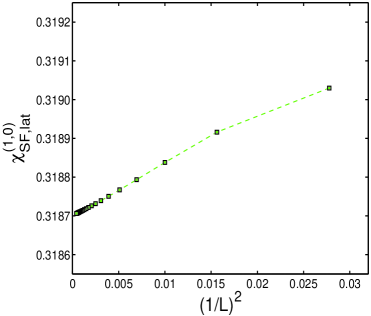
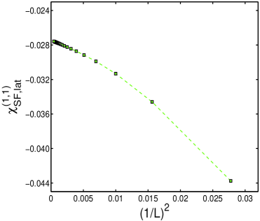
For the relation between the two schemes, we use the connection of the operators in the lattice minimal subtraction scheme (“lat”) and the MS¯¯MS{\rm\overline{MS\kern-0.50003pt}\kern 0.50003pt} scheme of dimensional regularization on the one hand and performed a 1-loop computation of the SF renormalization factor in the lattice regularization on the other hand. The latter, new, computation is detailed in App. A. Here we just quote the results and combine them to obtain γ1SFsubscriptsuperscript𝛾SF1\gamma^{\rm SF}_{1}.

At 1-loop order, the operator in the lattice minimal subtraction scheme is given by

𝒪spinlat(μ)=[1g02γ0ln(μa)]𝒪spinsuperscriptsubscript𝒪spinlat𝜇delimited-[]1superscriptsubscript𝑔02subscript𝛾0𝜇𝑎subscript𝒪spin\displaystyle{\cal O}_{\mathrm{spin}}^{\rm lat}(\mu)=[1-g_{0}^{2}\gamma_{0}\ln(\mu a)]{\cal O}_{\mathrm{spin}} (3.28)

with the bare operator 𝒪spinsubscript𝒪spin{\cal O}_{\mathrm{spin}} defined earlier. It is related to the operators in the SF scheme and the MS¯¯MS{\rm\overline{MS\kern-0.50003pt}\kern 0.50003pt} scheme by finite renormalizations,

𝒪spinSF(μ)=χSF,lat(glat2(μ))𝒪spinlat(μ),𝒪spinMS¯(μ)=χMS¯,lat(glat2(μ))𝒪spinlat(μ).formulae-sequencesuperscriptsubscript𝒪spinSF𝜇subscript𝜒SFlatsuperscriptsubscript𝑔lat2𝜇superscriptsubscript𝒪spinlat𝜇superscriptsubscript𝒪spin¯MS𝜇subscript𝜒¯MSlatsuperscriptsubscript𝑔lat2𝜇superscriptsubscript𝒪spinlat𝜇\displaystyle{\cal O}_{\mathrm{spin}}^{\rm SF}(\mu)=\chi_{\rm SF,lat}(g_{{\rm lat}}^{2}(\mu)){\cal O}_{\mathrm{spin}}^{\rm lat}(\mu)\,,\quad{\cal O}_{\mathrm{spin}}^{{\rm\overline{MS\kern-0.35002pt}\kern 0.35002pt}}(\mu)=\chi_{\rm{\rm\overline{MS\kern-0.35002pt}\kern 0.35002pt},lat}(g_{{\rm lat}}^{2}(\mu)){\cal O}_{\mathrm{spin}}^{\rm lat}(\mu)\,. (3.29)

For our purposes it suffices to know the expansions up to order g2superscript𝑔2g^{2},

χa,b(g2)=1+χa,b(1)g2+,subscript𝜒𝑎𝑏superscript𝑔21superscriptsubscript𝜒𝑎𝑏1superscript𝑔2\displaystyle\chi_{a,b}(g^{2})=1+\chi_{a,b}^{(1)}\,g^{2}+\ldots\,, (3.30)

where

χMS¯,lat(1)=0.3824superscriptsubscript𝜒¯MSlat10.3824\displaystyle\chi_{\rm{\rm\overline{MS\kern-0.35002pt}\kern 0.35002pt},lat}^{(1)}=0.3824 (3.31)

has been computed333Taking into account the discussion in [?], the value of e𝑒e should be reduced from e=24.48𝑒24.48e=24.48 in [?] to e=4.53𝑒4.53e=4.53. In the notation of [?] we have χMS¯,lat(1)=116π2[Cf(Dce+4π2)+CA(Da+DbDc/2)]superscriptsubscript𝜒¯MSlat1116superscript𝜋2delimited-[]subscript𝐶𝑓subscript𝐷𝑐𝑒4superscript𝜋2subscript𝐶𝐴subscript𝐷𝑎subscript𝐷𝑏subscript𝐷𝑐2\chi_{\rm{\rm\overline{MS\kern-0.35002pt}\kern 0.35002pt},lat}^{(1)}={1\over 16\pi^{2}}[C_{f}(D_{c}-e+4\pi^{2})+C_{A}(D_{a}+D_{b}-D_{c}/2)]. We thank Jonathan Flynn for clarifying this point. When numerical uncertainties are not written explicitly, they are estimated to be at most of order 2 on the last digit. by Flynn and Hill [?] and

χSF,lat(1)=0.3187016(1)0.027448(1)Nfsubscriptsuperscript𝜒1SFlat0.318701610.0274481subscript𝑁f\displaystyle\chi^{(1)}_{\rm SF,lat}=0.3187016(1)-0.027448(1)\,N_{\rm f} (3.32)

is obtained in App. A. These are combined to

χSF,MS¯(1)=χSF,lat(1)χMS¯,lat(1)=0.06370.0275Nf.superscriptsubscript𝜒SF¯MS1superscriptsubscript𝜒SFlat1superscriptsubscript𝜒¯MSlat10.06370.0275subscript𝑁f\displaystyle\chi_{\rm SF,{\rm\overline{MS\kern-0.35002pt}\kern 0.35002pt}}^{(1)}=\chi_{\rm SF,lat}^{(1)}-\chi_{\rm{\rm\overline{MS\kern-0.35002pt}\kern 0.35002pt},lat}^{(1)}=-0.0637-0.0275\,N_{\rm f}\,. (3.33)

Note that the Nfsubscript𝑁fN_{\rm f}-dependent part depends on the value θ𝜃\theta chosen for the spatial boundary conditions of the quark fields in eq. (3.23). The above result refers to θ=π/3𝜃𝜋3\theta=-\pi/3, for which the expectation values in eq. (3.23) can be shown to be real [?].

The last missing ingredient is the relation between the couplings, (at the same renormalization scale)

g¯SF2=χgg¯MS¯2,χg=1+χg(1)g¯MS¯2+O(g¯MS¯4),formulae-sequencesuperscriptsubscript¯𝑔SF2subscript𝜒gsuperscriptsubscript¯𝑔¯MS2subscript𝜒g1superscriptsubscript𝜒g1superscriptsubscript¯𝑔¯MS2𝑂superscriptsubscript¯𝑔¯MS4\bar{g}_{\rm SF}^{2}=\chi_{\rm g}\bar{g}_{{\rm\overline{MS\kern-0.35002pt}\kern 0.35002pt}}^{2},\qquad\chi_{\rm g}=1+\chi_{\rm g}^{(1)}\bar{g}_{{\rm\overline{MS\kern-0.35002pt}\kern 0.35002pt}}^{2}+O(\bar{g}_{{\rm\overline{MS\kern-0.35002pt}\kern 0.35002pt}}^{4})\,, (3.34)

with the 1-loop coefficient [?,?]

χg(1)=14π(c1,0+c1,1Nf),c1,0=1.25563(4),c1,1=0.039863formulae-sequencesuperscriptsubscript𝜒g114𝜋subscript𝑐10subscript𝑐11subscript𝑁fformulae-sequencesubscript𝑐101.255634subscript𝑐110.039863\chi_{\rm g}^{(1)}=-{1\over 4\pi}(c_{1,0}+c_{1,1}N_{\rm f})\,,\quad c_{1,0}=1.25563(4)\,,\;c_{1,1}=0.039863 (3.35)

for the SF-coupling defined at θ=π/5𝜃𝜋5\theta=\pi/5 [?].

Analogous to [?], where the discussion is carried through for the anomalous dimension of quark masses, we then obtain the desired result

γ1SF=γ1MS¯+2b0χSF,MS¯(1)γ0χg(1)=0.002360.00352Nf+0.00023Nf2.subscriptsuperscript𝛾SF1subscriptsuperscript𝛾¯MS12subscript𝑏0superscriptsubscript𝜒SF¯MS1subscript𝛾0superscriptsubscript𝜒g10.002360.00352subscript𝑁f0.00023superscriptsubscript𝑁f2\gamma^{\rm SF}_{1}=\gamma^{\overline{\rm MS}}_{1}+2b_{0}\,\chi_{\rm SF,{\rm\overline{MS\kern-0.35002pt}\kern 0.35002pt}}^{(1)}-\gamma_{0}\chi_{\rm g}^{(1)}=-0.00236-0.00352\,N_{\rm f}+0.00023\,N_{\rm f}^{2}\,. (3.36)

Our computation used the lattice regularization but the result is regularization independent.

4 Step scaling functions

4.1 Definition

The anomalous dimension, which we just obtained in 2-loop approximation, describes the change of the operator 𝒪spinSFsuperscriptsubscript𝒪spinSF{\cal O}_{\mathrm{spin}}^{\rm SF} under an infinitesimal change in the renormalization scale. For numerical, non-perturbative computations one considers finite changes of the scale, typically by a factor of two. These define the step scaling function σspin(u)subscript𝜎spin𝑢\sigma_{\rm spin}(u) via

𝒪spinSF(μ)=σspin(g¯2(1/μ))𝒪spinSF(2μ).superscriptsubscript𝒪spinSF𝜇subscript𝜎spinsuperscript¯𝑔21𝜇superscriptsubscript𝒪spinSF2𝜇{\cal O}_{\mathrm{spin}}^{\rm SF}(\mu)=\sigma_{\rm spin}(\bar{g}^{2}(1/\mu))\,{\cal O}_{\mathrm{spin}}^{\rm SF}(2\mu)\,. (4.37)

It is given by the continuum limit

σspin(u)=lima/L0Σspin(u,a/L)subscript𝜎spin𝑢subscript𝑎𝐿0subscriptΣspin𝑢𝑎𝐿\sigma_{\rm spin}(u)=\lim_{a/L\to 0}\Sigma_{\rm spin}(u,a/L) (4.38)

of the lattice step scaling function

Σspin(u,a/L)=ZspinSF(2L)ZspinSF(L)|g¯2(L)=u,m=0.subscriptΣspin𝑢𝑎𝐿evaluated-atsuperscriptsubscript𝑍spinSF2𝐿superscriptsubscript𝑍spinSF𝐿formulae-sequencesuperscript¯𝑔2𝐿𝑢𝑚0\Sigma_{\rm spin}(u,a/L)=\left.{Z_{\rm spin}^{\rm SF}(2L)\over Z_{\rm spin}^{\rm SF}(L)}\right|_{\bar{g}^{2}(L)=u\,,\;m=0}\,. (4.39)

Here g¯2(L)superscript¯𝑔2𝐿\bar{g}^{2}(L) denotes the SF coupling as before and the condition m=0𝑚0m=0 means that the renormalization condition is imposed at vanishing quark mass. In our numerical implementation the latter does not play a rôle since we work in the pure gauge theory. It is important to understand whether a given renormalization condition leads to small or large a𝑎a-effects. This determines whether the limit in eq. (4.38) can be taken by an extrapolation from the accessible lattices. A first understanding can be sought in perturbation theory.

4.2 Lattice artefacts in perturbation theory

We define the relative lattice artefacts as

δ(u,a/L)=Σspin(u,a/L)σspin(u)σspin(u)=δ1(a/L)u+O(u2).𝛿𝑢𝑎𝐿subscriptΣspin𝑢𝑎𝐿subscript𝜎spin𝑢subscript𝜎spin𝑢subscript𝛿1𝑎𝐿𝑢Osuperscript𝑢2\delta(u,a/L)={\Sigma_{\rm spin}(u,a/L)-\sigma_{\rm spin}(u)\over\sigma_{\rm spin}(u)}=\delta_{1}(a/L)\,u+{\rm O}(u^{2})\,. (4.40)

A term δ0(a/L)subscript𝛿0𝑎𝐿\delta_{0}(a/L) is absent since we defined ZspinSF(L)superscriptsubscript𝑍spinSF𝐿Z_{\rm spin}^{\rm SF}(L) such that it is one at tree-level for any value of a/L𝑎𝐿a/L. The 1-loop term may be expanded in Nfsubscript𝑁fN_{\rm f},

δ1(a/L)=δ1,0(a/L)+Nfδ1,1(a/L).subscript𝛿1𝑎𝐿subscript𝛿10𝑎𝐿subscript𝑁fsubscript𝛿11𝑎𝐿\delta_{1}(a/L)=\delta_{1,0}(a/L)+N_{\rm f}\,\delta_{1,1}(a/L)\,. (4.41)

With all improvement terms, including the boundary improvement term ctsubscript𝑐tc_{\rm t} [?], set to their proper perturbative values, the 1-loop cutoff effects turn out to be rather small. We show them in Table 1 for the Eichten-Hill action for the static quarks (W(x,0)=U(x,0)𝑊𝑥0𝑈𝑥0W(x,0)=U(x,0)), the plaquette gauge action and the O(a)O𝑎{\rm O}(a)-improved fermion action [?].

L/a𝐿𝑎L/a δ1,0(a/L)subscript𝛿10𝑎𝐿\delta_{1,0}(a/L) δ1,1(a/L)subscript𝛿11𝑎𝐿\delta_{1,1}(a/L)
6 -0.000236 0.013742
8 -0.000165 0.005791
10 -0.000106 0.003026
12 -0.000072 0.001876
14 -0.000051 0.001296
16 -0.000038 0.000956
Table 1: Lattice spacing effects of ΣspinsubscriptΣspin\Sigma_{\rm spin} in 1-loop perturbation theory, see text.

4.3 Non-perturbative results for Nf=0subscript𝑁f0N_{\rm f}=0

We carried out pure gauge theory simulations to determine ΣspinsubscriptΣspin\Sigma_{\rm spin} for different couplings u𝑢u, resolutions 1/12a/L1/6112𝑎𝐿161/12\leq a/L\leq 1/6 and also for different discretizations of the HQET action and the operator Fμνsubscript𝐹𝜇𝜈F_{\mu\nu}. Tables of the numerical results are found in App. B.
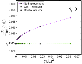
Refer to caption
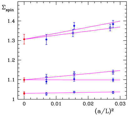
Figure 2: Examples of continuum extrapolations of ΣspinsubscriptΣspin\Sigma_{\rm spin} for u=𝑢absentu=1.243, 2.77 and 3.48. Filled symbols indicate that Fμνsubscript𝐹𝜇𝜈F_{\mu\nu} was defined as F^μνsubscript^𝐹𝜇𝜈\hat{F}_{\mu\nu} but with the link variables replaced by HYP2 links. The data at the largest coupling has ctsubscript𝑐tc_{\rm t} at 2-loop precision, otherwise it is set to the 1-loop value.

In Fig. 2 we show the a𝑎a-dependence for a few couplings and choices of discretizations. Lattice artefacts are moderate in general and a simple continuum extrapolation with an ansatz Σ=σ+(a/L)2ρΣ𝜎superscript𝑎𝐿2𝜌\Sigma=\sigma+(a/L)^{2}\,\rho, separately for each value of u𝑢u seems justified.444We also checked other extrapolations, see e.g. [?,?]. They give compatible results. In cases where more than one discretization was simulated at the same value of u𝑢u, a constrained extrapolation (common σ𝜎\sigma but discretization-dependent ρ𝜌\rho) was performed. This simple analysis yields the continuum step scaling functions in Table 2.

u𝑢u σspin(u)subscript𝜎spin𝑢\sigma_{\rm spin}(u) ρ(u)𝜌𝑢\rho(u) action F^μνsubscript^𝐹𝜇𝜈\hat{F}_{\mu\nu} n𝑛n-loop ctsubscript𝑐tc_{\rm t}
0.8873 1.0235(68) 0.02(36)
0.9944 1.025(11) -0.15(53) EH
1.2430 1.0302(82) 0.24(42)
1.3293 1.043(12) -0.66(55) EH
1.5553 1.0418(89) 0.27(43)
1.8811 1.075(11) -0.44(52)
2.1000 1.052(14) 1.15(69)
2.4484 1.089(14) -0.31(68)
1.60(60)
2.770 1.099(11)
-0.01(55) HYP2
3.480 1.300(34) 5.2(1.6) HYP2
3.480 1.308(29) 3.0(1.4) HYP2 2
2.1(1.2) 2
3.480 1.306(25)
3.1(1.3) HYP2 2
Table 2: Continuum step scaling function σspinsubscript𝜎spin\sigma_{\rm spin} and coefficients of (a/L)2superscript𝑎𝐿2(a/L)^{2} in the continuum extrapolations. The standard discretization is the HYP2 action of [?], the clover leaf operator F^μνsubscript^𝐹𝜇𝜈\hat{F}_{\mu\nu} and the 1-loop value of ctsubscript𝑐tc_{\rm t}. Deviations from this rule are indicated: EH refers to the Eichten-Hill static action and the label HYP2 in the column F^μνsubscript^𝐹𝜇𝜈\hat{F}_{\mu\nu} means that the links appearing in F^μνsubscript^𝐹𝜇𝜈\hat{F}_{\mu\nu} are replaced by HYP2 links.

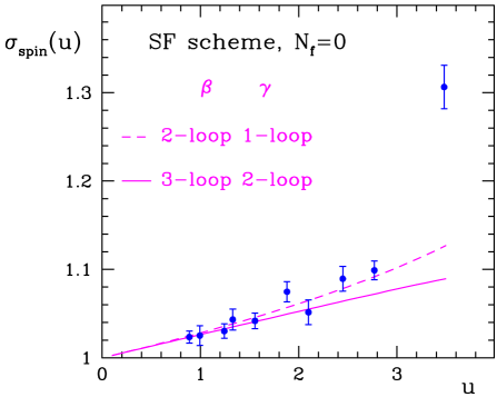
A good agreement with perturbation theory is seen at weak couplings, say g¯2<2superscript¯𝑔22\bar{g}^{2}<2, where, however, the non-perturbative results are not accurate enough to distinguish between the 2-loop anomalous dimension and the 1-loop one. On the other hand, for couplings g¯23superscript¯𝑔23\bar{g}^{2}\approx 3 perturbation theory breaks down entirely and the inclusion of the 2-loop anomalous dimension brings the perturbative curves even further away from the MC results.
Refer to caption
Figure 3: The step scaling function compared to the perturbative prediction obtained by integration of the perturbative RG equations, truncating the β𝛽\beta function at 3(2)-loop order and the anomalous dimension at 2(1)-loop order.

5 Non-perturbative scale dependence for Nf=0subscript𝑁f0N_{\rm f}=0

Through an iterative application of the (inverse) step scaling function we now determine the non-perturbative scale dependence of the operator in the SF scheme. We first represent the numerical data of Table 2 as well as the data for the step scaling function of the coupling, σ(u)𝜎𝑢\sigma(u) (Table A.2 of [?] and Table 4 of [?]) by smooth interpolations

σ(u)𝜎𝑢\displaystyle\sigma(u) =\displaystyle= u+i=04siui+2,𝑢superscriptsubscript𝑖04subscript𝑠𝑖superscript𝑢𝑖2\displaystyle u+\sum_{i=0}^{4}s_{i}\,u^{i+2}\,, (5.42)
σspin(u)subscript𝜎spin𝑢\displaystyle\sigma_{\rm spin}(u) =\displaystyle= 1+m0u+m1u2+m2u31subscript𝑚0𝑢subscript𝑚1superscript𝑢2subscript𝑚2superscript𝑢3\displaystyle 1+m_{0}\,u+m_{1}\,u^{2}+m_{2}\,u^{3}\, (5.43)

for u2.8𝑢2.8u\leq 2.8. Here s0=2ln(2)b0,s1=s02+2ln(2)b1,m0=ln(2)γ0formulae-sequencesubscript𝑠022subscript𝑏0formulae-sequencesubscript𝑠1superscriptsubscript𝑠0222subscript𝑏1subscript𝑚02subscript𝛾0s_{0}=2\ln(2)\,b_{0}\,,\;s_{1}=s_{0}^{2}+2\ln(2)\,b_{1}\,,\;m_{0}=\ln(2)\,\gamma_{0} are fixed by perturbation theory, while the other coefficients are free fit parameters. With these parameterizations we then solve the recursions 555 ΦΦ\Phi stands for any matrix element of the operator 𝒪spinsubscript𝒪spin{\cal O}_{\mathrm{spin}}, for example the matrix element λ2subscript𝜆2\lambda_{2}.

u0=g¯2(Lmax)=3.48,σ(uk+1)=uk,formulae-sequencesubscript𝑢0superscript¯𝑔2subscript𝐿max3.48𝜎subscript𝑢𝑘1subscript𝑢𝑘\displaystyle u_{0}=\bar{g}^{2}(L_{\rm max})=3.48\,,\quad\sigma(u_{k+1})=u_{k}\,, \displaystyle\Rightarrow g¯2(2kLmax)=uk,superscript¯𝑔2superscript2𝑘subscript𝐿maxsubscript𝑢𝑘\displaystyle\bar{g}^{2}(2^{-k}L_{\rm max})=u_{k}\,,
w0=1,wk+1=wk/σspin(uk+1)formulae-sequencesubscript𝑤01subscript𝑤𝑘1subscript𝑤𝑘subscript𝜎spinsubscript𝑢𝑘1\displaystyle w_{0}=1\,,\quad w_{k+1}=w_{k}/\sigma_{\rm spin}(u_{k+1}) \displaystyle\Rightarrow ΦSF(2k/Lmax)ΦSF(1/Lmax)=wk.subscriptΦSFsuperscript2𝑘subscript𝐿maxsubscriptΦSF1subscript𝐿maxsubscript𝑤𝑘\displaystyle{\Phi_{\rm SF}(2^{k}/L_{\rm max})\over\Phi_{\rm SF}(1/L_{\rm max})}=w_{k}\,.

Errors are propagated through the parameterization and recursion and it is checked that changing the number of fit parameters in eq. (5.42) and eq. (5.43) does not alter the results significantly. Next we apply

ΦRGIΦSF(μ)=[ 2b0g¯2(μ)]γ0/2b0exp{0g¯(μ)dg[γSF(g)βSF(g)γ0b0g]}subscriptΦRGIsubscriptΦSF𝜇superscriptdelimited-[]2subscript𝑏0superscript¯𝑔2𝜇subscript𝛾02subscript𝑏0superscriptsubscript0¯𝑔𝜇differential-d𝑔delimited-[]superscript𝛾SF𝑔superscript𝛽SF𝑔subscript𝛾0subscript𝑏0𝑔{\Phi_{\rm RGI}\over\Phi_{\rm SF}(\mu)}=\left[\,2b_{0}\bar{g}^{2}(\mu)\,\right]^{-\gamma_{0}/2b_{0}}\exp\left\{-\int_{0}^{\bar{g}(\mu)}{\rm d}g\left[\,{\gamma^{\rm SF}(g)\over\beta^{\rm SF}(g)}-{\gamma_{0}\over b_{0}g}\,\right]\right\}\, (5.45)

for μ=2k/Lmax𝜇superscript2𝑘subscript𝐿max\mu=2^{k}/L_{\rm max} and the perturbative approximations to the β𝛽\beta-function and anomalous dimensions and obtain ΦSF(1/Lmax)/ΦRGIsubscriptΦSF1subscript𝐿maxsubscriptΦRGI\Phi_{\rm SF}(1/L_{\rm max})/\Phi_{\rm RGI}. Finally we form ΦSF(1/(2Lmax))/ΦRGI=σspin(u0)ΦSF(1/Lmax)/ΦRGIsubscriptΦSF12subscript𝐿maxsubscriptΦRGIsubscript𝜎spinsubscript𝑢0subscriptΦSF1subscript𝐿maxsubscriptΦRGI\Phi_{\rm SF}(1/(2L_{\rm max}))/\Phi_{\rm RGI}=\sigma_{\rm spin}(u_{0})\,\Phi_{\rm SF}(1/L_{\rm max})/\Phi_{\rm RGI} with σspin(u0)subscript𝜎spinsubscript𝑢0\sigma_{\rm spin}(u_{0}) from Table 2. For not too small k𝑘k, the final result is independent of it; the use of perturbation theory is safe in that region. Taking k=6𝑘6k=6, the 2-loop approximation for the anomalous dimension and the 3-loop approximation for the β𝛽\beta-function we arrive at

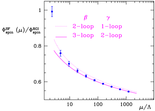
ΦSF(μ)/ΦRGIsubscriptΦSF𝜇subscriptΦRGI\displaystyle\Phi_{\rm SF}(\mu)/\Phi_{\rm RGI} =\displaystyle= 0.759(17),at μ=1/Lmax,0.75917at 𝜇1subscript𝐿max\displaystyle 0.759(17)\,,\quad\text{at }\mu=1/L_{\rm max}\,, (5.46)
ΦSF(μ)/ΦRGIsubscriptΦSF𝜇subscriptΦRGI\displaystyle\Phi_{\rm SF}(\mu)/\Phi_{\rm RGI} =\displaystyle= 0.992(29),at μ=1/(2Lmax).0.99229at 𝜇12subscript𝐿max\displaystyle 0.992(29)\,,\quad\text{at }\mu=1/(2L_{\rm max})\,. (5.47)

Figure 4 compares the non-perturbative running of 𝒪spinsubscript𝒪spin{\cal O}_{\mathrm{spin}} to perturbation theory.

Refer to caption
Figure 4: Scale dependence of 𝒪spinsubscript𝒪spin{\cal O}_{\mathrm{spin}} in the SF scheme.

5.1 The relation of bare and renormalization group invariant operator

The universal result eq. (5.47) has to be combined with values of ZspinSF(L)superscriptsubscript𝑍spinSF𝐿Z_{\rm spin}^{\rm SF}(L) at L=2Lmax=1.436r0𝐿2subscript𝐿max1.436subscript𝑟0L=2L_{\rm max}=1.436\,r_{0} [?] which depend on the bare coupling and lattice action, to form

ZspinRGI=ZspinSF(L)×ΦRGIΦSF(1/L)superscriptsubscript𝑍spinRGIsuperscriptsubscript𝑍spinSF𝐿subscriptΦRGIsubscriptΦSF1𝐿Z_{\rm spin}^{\rm RGI}=Z_{\rm spin}^{\rm SF}(L)\times{\Phi_{\rm RGI}\over\Phi_{\rm SF}(1/L)} (5.48)

for the respective action. The numerical values of Table 3 are well represented by

ZspinSF(2Lmax)superscriptsubscript𝑍spinSF2subscript𝐿max\displaystyle Z_{\rm spin}^{\rm SF}(2L_{\rm max}) =\displaystyle= 2.58+0.14(β6)0.27(β6)2EH action,2.580.14𝛽60.27superscript𝛽62EH action\displaystyle 2.58+0.14\,(\beta-6)-0.27\,(\beta-6)^{2}\,\quad\text{EH action}\,, (5.49)
ZspinSF(2Lmax)superscriptsubscript𝑍spinSF2subscript𝐿max\displaystyle Z_{\rm spin}^{\rm SF}(2L_{\rm max}) =\displaystyle= 2.59+0.11(β6)0.34(β6)2HYP2 action.2.590.11𝛽60.34superscript𝛽62HYP2 action\displaystyle 2.59+0.11\,(\beta-6)-0.34\,(\beta-6)^{2}\,\quad\text{HYP2 action}\,. (5.50)

These interpolations may be used in the interval 6.0β6.56.0𝛽6.56.0\leq\beta\leq 6.5 with an error of about 1%. While this error ought to be taken into account before the continuum extrapolation of the renormalized matrix elements, the uncertainty in eq. (5.47) applies additionally in the continuum limit.

β𝛽\beta L/a𝐿𝑎L/a action ZspinSFsuperscriptsubscript𝑍spinSFZ_{\rm spin}^{\rm SF}
6.0219 8 EH 2.585(19)
6.1628 10 EH 2.602(24)
6.2885 12 EH 2.602(24)
6.3992 14 EH 2.589(29)
6.4956 16 EH 2.593(35)
6.0219 8 HYP2 2.593(21)
6.1628 10 HYP2 2.589(26)
6.2885 12 HYP2 2.589(26)
6.3992 14 HYP2 2.585(21)
6.4956 16 HYP2 2.553(22)
Table 3: Renormalization factor at the matching scale. In all cases F^μνsubscript^𝐹𝜇𝜈\hat{F}_{\mu\nu} is the standard clover operator.

6 First applications

We illustrate the usefulness of our result with two sample applications.

6.1 Spin splitting

First we take numbers for the bare λ2subscript𝜆2\lambda_{2} which have been reported in the literature. Unfortunately they exist only for β=6.0𝛽6.0\beta=6.0, which corresponds to a0.1fm𝑎0.1fma\approx 0.1\,{\rm fm}. The more recent evaluations are (the light quark has the mass of the strange quark)

Ref. [?]: a2λ2bare=0.0100(19),superscript𝑎2superscriptsubscript𝜆2bare0.010019\displaystyle a^{2}\lambda_{2}^{\rm bare}=0.0100(19)\,, (6.51)
Ref. [?]: a2λ2bare=0.0138(15).superscript𝑎2superscriptsubscript𝜆2bare0.013815\displaystyle a^{2}\lambda_{2}^{\rm bare}=0.0138(15)\,. (6.52)

The authors of [?,?] then estimate the mass splitting as

Ref. [?]: Δm2=0.28(6)(?)GeV2,Δsuperscript𝑚20.286?superscriptGeV2\displaystyle\Delta m^{2}=0.28(6)(?)\,{\rm GeV}^{2}\,, (6.53)
Ref. [?]: Δm2=0.36(4)(?)GeV2,Δsuperscript𝑚20.364?superscriptGeV2\displaystyle\Delta m^{2}=0.36(4)(?)\,{\rm GeV}^{2}\,, (6.54)

where the renormalization factor is taken from perturbation theory using a boosted coupling [?] and by tadpole improved perturbation theory [?]666Also somewhat different values for the lattice spacing were used by the two groups.. With Cspin(Mb/ΛMS¯)=1.15subscript𝐶spinsubscript𝑀bsubscriptΛ¯MS1.15C_{\rm spin}(M_{{\rm b}}/\Lambda_{\rm\overline{MS\kern-0.35002pt}\kern 0.35002pt})=1.15, Mb=6.76(9)GeVsubscript𝑀b6.769GeVM_{{\rm b}}=6.76(9)\,{\rm GeV} [?,?] and ZspinRGI=2.6,a=1/(2GeV)formulae-sequencesuperscriptsubscript𝑍spinRGI2.6𝑎12GeVZ_{\rm spin}^{\rm RGI}=2.6\,,a=1/(2\,{\rm GeV}) we find from eq. (1.6)

Ref. [?] and NP ZspinRGIsuperscriptsubscript𝑍spinRGIZ_{\rm spin}^{\rm RGI}: Δm2=0.38(7)(?)GeV2,Δsuperscript𝑚20.387?superscriptGeV2\displaystyle\Delta m^{2}=0.38(7)(?)\,{\rm GeV}^{2}\,, (6.55)
Ref. [?] and NP ZspinRGIsuperscriptsubscript𝑍spinRGIZ_{\rm spin}^{\rm RGI}: Δm2=0.53(6)(?)GeV2.Δsuperscript𝑚20.536?superscriptGeV2\displaystyle\Delta m^{2}=0.53(6)(?){\rm GeV}^{2}\,. (6.56)

In all these estimates the additional uncertainty marked as (?) refers to lattice artefacts, namely the fact that a continuum limit has not been taken, and of course to the missing dynamical quark determinant. The experimental mass splitting is Δm2=0.497GeV2Δsuperscript𝑚20.497superscriptGeV2\Delta m^{2}=0.497\,{\rm GeV}^{2}.

6.2 Renormalization factor for spin-dependent potentials

In phenomenological applications of the spin-dependent potentials, the standard renormalization scheme is MS¯¯MS{\rm\overline{MS\kern-0.50003pt}\kern 0.50003pt}, as in [?,?,?,?]. We apply eq. (5.45) in the MS¯¯MS{\rm\overline{MS\kern-0.50003pt}\kern 0.50003pt} scheme with Nf=0subscript𝑁f0N_{\rm f}=0, ΛMS¯(0)=238MeVsuperscriptsubscriptΛ¯MS0238MeV\Lambda_{{\rm\overline{MS\kern-0.35002pt}\kern 0.35002pt}}^{(0)}=238\,{\rm MeV} [?], the 4-loop β𝛽\beta-function and the 2-loop anomalous dimension. This yields

ZspinMS¯(2GeV)superscriptsubscript𝑍spin¯MS2GeV\displaystyle Z_{\rm spin}^{{\rm\overline{MS\kern-0.35002pt}\kern 0.35002pt}}(2\,{\rm GeV}) =\displaystyle= 0.756(18)×ZspinRGI(g0),0.75618superscriptsubscript𝑍spinRGIsubscript𝑔0\displaystyle 0.756(18)\times Z_{\rm spin}^{\rm RGI}(g_{0})\,, (6.57)
ZspinMS¯(4GeV)superscriptsubscript𝑍spin¯MS4GeV\displaystyle Z_{\rm spin}^{{\rm\overline{MS\kern-0.35002pt}\kern 0.35002pt}}(4\,{\rm GeV}) =\displaystyle= 0.706(13)×ZspinRGI(g0),0.70613superscriptsubscript𝑍spinRGIsubscript𝑔0\displaystyle 0.706(13)\times Z_{\rm spin}^{\rm RGI}(g_{0})\,, (6.58)

where the cited error bar is half of the change when one uses the 1-loop anomalous dimension instead. Remember from Sect. 3 that the square of this renormalization factor enters the potentials. As an illustration, for the standard Eichten-Hill action for the static quarks, at g0=1subscript𝑔01g_{0}=1 (β=6.0𝛽6.0\beta=6.0), we then have ZMS¯(2GeV)0.756×2.58×0.99=1.93subscript𝑍¯MS2GeV0.7562.580.991.93Z_{{\rm\overline{MS\kern-0.35002pt}\kern 0.35002pt}}(2\,{\rm GeV})\approx 0.756\times 2.58\times 0.99=1.93 or a somewhat smaller number at larger μ𝜇\mu. One can compare this at g0=1subscript𝑔01g_{0}=1 to the renormalization factors used in [?]. A tree-level tadpole-improved factor is Ztad=1.684subscript𝑍tad1.684Z_{\rm tad}=1.684 and the Huntley-Michael factor777The prescription of [?] yields a small r𝑟r-dependence, which is not present in the standard renormalization of local operators. is around ZHM=1.62subscript𝑍HM1.62Z_{\rm HM}=1.62. Since a renormalization scheme and scale are not specified in these procedures, there is no reason to expect a closer agreement.

7 Conclusions

We have presented yet another example that the non-perturbative renormalization programme using recursive finite size techniques [?,?] can be carried out also in difficult cases. Four-fermion operators were renormalized successfully in [?,?], and those containing static quarks in [?,?]. Here we have treated the case of an operator with static quarks and gluon fields.

In several cases quite significant deviations from perturbation theory had already been observed at intermediate to low renormalization scales [?,?,?], but the present case is the strongest example in that respect (Fig. 3, Fig. 4).

Our example in the previous section illustrates that the non-perturbative ZspinRGIsuperscriptsubscript𝑍spinRGIZ_{\rm spin}^{\rm RGI} has a rather big effect. Although the quenched estimates for Δm2=mBs2mBs2Δsuperscript𝑚2superscriptsubscript𝑚superscriptsubscriptBs2superscriptsubscript𝑚subscriptBs2\Delta m^{2}=m_{\rm B_{\rm s}^{*}}^{2}-m_{\rm B_{\rm s}}^{2} are in rough agreement with the experimental mass splitting Δm2=0.497GeV2Δsuperscript𝑚20.497superscriptGeV2\Delta m^{2}=0.497\,{\rm GeV}^{2} after the non-perturbative ZspinRGIsuperscriptsubscript𝑍spinRGIZ_{\rm spin}^{\rm RGI} is used, it now remains to improve the precision of the bare matrix element as well as to obtain it at smaller lattice spacings in order to see whether the quenched approximation does indeed give a reasonable estimate of the spin splitting. We also emphasize that there is a remaining uncertainty in the use of (continuum) perturbation theory for Cspin(Mb/ΛMS¯)subscript𝐶spinsubscript𝑀bsubscriptΛ¯MSC_{\rm spin}(M_{{\rm b}}/\Lambda_{\rm\overline{MS\kern-0.35002pt}\kern 0.35002pt}). This can be significantly reduced by a computation of the associated 3-loop anomalous dimension, but also an entirely non-perturbative matching of HQET and QCD is promising [?,?].

Acknowledgements. We acknowledge useful discussions with N. Brambilla, M. Della Morte, J. Flynn, P. Marquard, J. Pilcum, J. Soto, M. Steinhauser, A. Vairo, S. Takeda and U. Wolff. We thank NIC for allocating computer time on the APEmille computers at DESY Zeuthen to this project and the APE group for its help. This work is supported by the Deutsche Forschungsgemeinschaft in the SFB/TR 09 , by the European community through EU Contract No. MRTN-CT-2006-035482, “FLAVIAnet” and by funds provided by the U.S. Department of Energy under cooperative research agreement DE-FC02-94ER40818.

Appendix A One-loop computation

Our aim is to compute the expectation value of a general Wilson loop at one-loop order in the Schrödinger functional (SF), bearing in mind that we are finally interested in the computation of the expectation value of a clover operator F^μνsubscript^𝐹𝜇𝜈\hat{F}_{\mu\nu} inserted into a Polyakov loop, enabling us to obtain the two-loop anomalous dimension of the chromo-magnetic operator in the SF scheme from its value in the lat scheme. Due to the space-time locality of such an observable, it will be advantageous to compute the gluon loops in x𝑥x space, while the contribution of tadpoles is proportional to the zero-momentum gluon propagator. Quite a lot of notation will be introduced, but the formulae presented here are suitable for the automated computation of arbitrary Wilson loops.

The lattice spacing is set to one in this appendix. Space-time indices run from 1 to 4, the latter being associated with time. For everything else we reuse the notation of [?], referred to as (K) in what follows, except that a twiddle on the color components of gluon, ghost and quark fields is dropped. The reader is assumed to be familiar with chapters 3, 4 and 5 of (K). Up to one-loop order, the observable 𝒪𝒪{\cal O} has the perturbative expansion (K:4.39)

𝒪=𝒪(0)+g02[𝒪(2)0𝒪(1)S(1)0]+O(g04),delimited-⟨⟩𝒪superscript𝒪0superscriptsubscript𝑔02delimited-[]subscriptdelimited-⟨⟩superscript𝒪20subscriptdelimited-⟨⟩superscript𝒪1superscript𝑆10Osuperscriptsubscript𝑔04\langle{\cal O}\rangle={\cal O}^{(0)}+g_{0}^{2}\left[\langle{\cal O}^{(2)}\rangle_{0}-\langle{\cal O}^{(1)}S^{(1)}\rangle_{0}\right]+{\rm O}(g_{0}^{4}), (A.59)

where 0subscriptdelimited-⟨⟩0\langle\dots\rangle_{0} is the expectation value with respect to the free part S(0)superscript𝑆0S^{(0)} of the action and 𝒪(k)superscript𝒪𝑘{\cal O}^{(k)} is defined by 𝒪=𝒪(0)+𝒪(1)g0+𝒪(2)g02+𝒪superscript𝒪0superscript𝒪1subscript𝑔0superscript𝒪2superscriptsubscript𝑔02{\cal O}={\cal O}^{(0)}+{\cal O}^{(1)}g_{0}+{\cal O}^{(2)}g_{0}^{2}+\dots.

The (constant, Abelian) background field induced by the non-trivial boundary conditions takes the value Vμ(x)subscript𝑉𝜇𝑥V_{\mu}(x). We use the basis of the su(3)𝑠𝑢3su(3) Lie algebra

qμ(x)=a=18qμa(x)Iasubscript𝑞𝜇𝑥superscriptsubscript𝑎18subscriptsuperscript𝑞𝑎𝜇𝑥superscript𝐼𝑎q_{\mu}(x)=\sum_{a=1}^{8}q^{a}_{\mu}(x)I^{a} (A.60)

defined in (K:App. A) as well as the Fourier representation

q4a(x)superscriptsubscript𝑞4𝑎𝑥\displaystyle q_{4}^{a}(x) =\displaystyle= 1L3𝐩ei𝐩𝐱q4a(𝐩,x4).1superscript𝐿3subscript𝐩superscript𝑒𝑖𝐩𝐱superscriptsubscript𝑞4𝑎𝐩subscript𝑥4\displaystyle\hbox{$1\over L^{3}$}\sum_{\bf p}e^{i{\bf p}\cdot{\bf x}}~{}q_{4}^{a}({\bf p},x_{4}). (A.61)
qka(x)superscriptsubscript𝑞𝑘𝑎𝑥\displaystyle q_{k}^{a}(x) =\displaystyle= 1L3𝐩ei𝐩𝐱ei(pk+ϕa(x4))/2qka(𝐩,x4).1superscript𝐿3subscript𝐩superscript𝑒𝑖𝐩𝐱superscript𝑒𝑖subscript𝑝𝑘subscriptitalic-ϕ𝑎subscript𝑥42superscriptsubscript𝑞𝑘𝑎𝐩subscript𝑥4\displaystyle\hbox{$1\over L^{3}$}\sum_{\bf p}e^{i{\bf p}\cdot{\bf x}}~{}e^{i(p_{k}+\phi_{a}(x_{4}))/2}q_{k}^{a}({\bf p},x_{4}). (A.62)

The gluon propagator in mixed representation used by (K) has the form

qμa(𝐩,x4)qνb(𝐩,y4)0=δba¯L3δ𝐩+𝐩Dμνa(𝐩;x4,y4).subscriptdelimited-⟨⟩superscriptsubscript𝑞𝜇𝑎𝐩subscript𝑥4superscriptsubscript𝑞𝜈𝑏superscript𝐩subscript𝑦40subscript𝛿𝑏¯𝑎superscript𝐿3subscript𝛿𝐩superscript𝐩superscriptsubscript𝐷𝜇𝜈𝑎𝐩subscript𝑥4subscript𝑦4\langle q_{\mu}^{a}({\bf p},x_{4})~{}q_{\nu}^{b}({\bf p}^{\prime},y_{4})\rangle_{0}=\delta_{b\bar{a}}L^{3}\delta_{{\bf p}+{\bf p^{\prime}}}~{}D_{\mu\nu}^{a}({\bf p};x_{4},y_{4}). (A.63)

Kronecker symbols such as δ𝐩subscript𝛿𝐩\delta_{\bf p} or δμ4subscript𝛿𝜇4\delta_{\mu-4} carrying a single index are shorthands for δ𝐩,𝟎subscript𝛿𝐩0\delta_{\bf p,0} and δμ,4subscript𝛿𝜇4\delta_{\mu,4} respectively.

A.1 Parameterization of the observable

In order to compute the expectation value of an arbitrary Wilson loop at one-loop order, we parameterize the loop by a starting point x(start)superscript𝑥startx^{({\rm start})} and an ordered list \vec{\ell} of length \ell. The entries of the list are directions μisuperscriptsubscript𝜇𝑖\mu_{i}^{\vec{\ell}}, i=1,,𝑖1i=1,\dots,\ell. These directions take non-zero integer values between 44-4 and +44+4. An electric plaquette in the (03)03(03) plane is thus parameterized by =(3434)3434\vec{\ell}=(3~{}~{}4~{}~{}-3~{}~{}-4). Clearly the loop is closed if and only if each integer appears as many times with the ++ sign as it does with the - sign (modulo L𝐿L for the space directions). We normally drop the \vec{\ell} in μisuperscriptsubscript𝜇𝑖\mu_{i}^{\vec{\ell}} since we will be dealing only with one path at a time.

The sequence of points the loop goes through is obtained as follows,

x(1)=x(start)x(i+1)=x(i)+μ^i,i=1,,1.formulae-sequencesuperscript𝑥1superscript𝑥startformulae-sequencesuperscript𝑥𝑖1superscript𝑥𝑖subscript^𝜇𝑖𝑖11x^{(1)}=x^{({\rm start})}\qquad x^{(i+1)}=x^{(i)}~{}+~{}\hat{\mu}_{i},\quad i=1,\dots,\ell-1. (A.64)

μ^=sign(μ)|μ|^^𝜇sign𝜇^𝜇\hat{\mu}={\rm sign}(\mu)\widehat{|\mu|} are unit vectors pointing in the four ±plus-or-minus\pm directions of the lattice. We identify 4^=0^^4^0\hat{4}=\hat{0}. At tree-level, the expectation value of the Wilson loop is

W[V]=i=1V(x(i),μi).subscript𝑊delimited-[]𝑉superscriptsubscriptproduct𝑖1𝑉superscript𝑥𝑖subscript𝜇𝑖W_{\vec{\ell}}[V]=\prod_{i=1}^{\ell}V(x^{(i)},\mu_{i}). (A.65)

In general, for any 4-vector we introduce negative-index components

pμ=pμ.subscript𝑝𝜇subscript𝑝𝜇p_{-\mu}=-p_{\mu}. (A.66)

Because of the way the path is parameterized, for any link variable we introduce negative-index components by imposing

U(x,μ)=U(x+μ^,μ),qμa(x)=qμa(x+μ^).formulae-sequence𝑈𝑥𝜇superscript𝑈𝑥^𝜇𝜇superscriptsubscript𝑞𝜇𝑎𝑥superscriptsubscript𝑞𝜇𝑎𝑥^𝜇U(x,\mu)=U^{\dagger}(x+\hat{\mu},-\mu),\qquad q_{\mu}^{a}(x)=-q_{-\mu}^{a}(x+\hat{\mu}). (A.67)

The Fourier representation is now defined for all μ𝜇\mu as follows,

qμa(x)=1L3𝐩ei𝐩𝐱eiθa(𝐩,x4,μ)qμa(𝐩,x4)superscriptsubscript𝑞𝜇𝑎𝑥1superscript𝐿3subscript𝐩superscript𝑒𝑖𝐩𝐱superscript𝑒𝑖subscript𝜃𝑎𝐩subscript𝑥4𝜇superscriptsubscript𝑞𝜇𝑎𝐩subscript𝑥4q_{\mu}^{a}(x)=\hbox{$1\over L^{3}$}\sum_{\bf p}e^{i{\bf p}\cdot{\bf x}}~{}e^{i\theta_{a}({\bf p},x_{4},\mu)}~{}q_{\mu}^{a}({\bf p},x_{4}) (A.68)

where

qμa(𝐩,x4)=q|μ|a(𝐩,x4δμ+4)superscriptsubscript𝑞𝜇𝑎𝐩subscript𝑥4superscriptsubscript𝑞𝜇𝑎𝐩subscript𝑥4subscript𝛿𝜇4q_{\mu}^{a}({\bf p},x_{4})=q_{|\mu|}^{a}({\bf p},x_{4}-\delta_{\mu+4}) (A.69)

and

eiθa(𝐩,x4,μ)superscript𝑒𝑖subscript𝜃𝑎𝐩subscript𝑥4𝜇\displaystyle e^{i\theta_{a}({\bf p},x_{4},\mu)} =\displaystyle= {1ifμ=4ei(pk+ϕa(x4))/2ifμ=kei(pk+ϕa(x4))/2ifμ=k1ifμ=4cases1if𝜇4superscript𝑒𝑖subscript𝑝𝑘subscriptitalic-ϕ𝑎subscript𝑥42if𝜇𝑘superscript𝑒𝑖subscript𝑝𝑘subscriptitalic-ϕ𝑎subscript𝑥42if𝜇𝑘1if𝜇4\displaystyle\left\{\begin{array}[]{l@{\qquad}l}1&{\rm if}~{}\mu=4\\ e^{i(p_{k}+\phi_{a}(x_{4}))/2}&{\rm if}~{}\mu=k\\ -e^{i(-p_{k}+\phi_{a}(x_{4}))/2}&{\rm if}~{}\mu=-k\\ -1&{\rm if}~{}\mu=-4\end{array}\right. (A.74)
=\displaystyle= sign(μ)(δ|μ|4+(1δ|μ|4)ei(pμ+ϕa(x4))/2).sign𝜇subscript𝛿𝜇41subscript𝛿𝜇4superscript𝑒𝑖subscript𝑝𝜇subscriptitalic-ϕ𝑎subscript𝑥42\displaystyle{\rm sign}(\mu)\left(\delta_{|\mu|-4}+(1-\delta_{|\mu|-4})e^{i(p_{\mu}+\phi_{a}(x_{4}))/2}\right). (A.75)

With these notations we have

qμa(𝐩,x4)qνb(𝐩,y4)=δba¯L3δ𝐩+𝐩D|μ||ν|a(𝐩;x4δμ+4;y4δν+4).delimited-⟨⟩superscriptsubscript𝑞𝜇𝑎𝐩subscript𝑥4superscriptsubscript𝑞𝜈𝑏superscript𝐩subscript𝑦4subscript𝛿𝑏¯𝑎superscript𝐿3subscript𝛿𝐩superscript𝐩superscriptsubscript𝐷𝜇𝜈𝑎𝐩subscript𝑥4subscript𝛿𝜇4subscript𝑦4subscript𝛿𝜈4\langle q_{\mu}^{a}({\bf p},x_{4})q_{\nu}^{b}({\bf p^{\prime}},y_{4})\rangle=\delta_{b\bar{a}}L^{3}\delta_{{\bf p}+{\bf p^{\prime}}}D_{|\mu||\nu|}^{a}\left({\bf p};x_{4}-\delta_{\mu+4};y_{4}-\delta_{\nu+4}\right). (A.76)

A.2 Tadpoles: 𝒪(1)S(1)0subscriptdelimited-⟨⟩superscript𝒪1superscript𝑆10\langle{\cal O}^{(1)}S^{(1)}\rangle_{0}

The terms considered in this subsection owe their existence to the non-vanishing background field. Since the latter is diagonal, the V𝑉V matrices all commute two-by-two and we have

tr{W(1)}=j=1tr{qμj(x(j))W[V]}.trsuperscriptsubscript𝑊1superscriptsubscript𝑗1trsubscript𝑞subscript𝜇𝑗superscript𝑥𝑗subscript𝑊delimited-[]𝑉\,\hbox{tr}\,\{W_{\vec{\ell}}^{(1)}\}=\sum_{j=1}^{\ell}\,\hbox{tr}\,\{q_{\mu_{j}}(x^{(j)})~{}W_{\vec{\ell}}[V]\}. (A.77)

The three contributions to S(1)superscript𝑆1S^{(1)} (coming from the gauge, ghost and quark terms) are given by eqs. (K:5.64,5.72) and for the quarks eqs. (K:5.76,5.82). After a short calculation one finds

tr{W(1)}S(1)0=a{3,8}μ=13u4α,μa(u4)Tμa(u4),subscriptdelimited-⟨⟩trsuperscriptsubscript𝑊1superscript𝑆10subscript𝑎38superscriptsubscript𝜇13subscriptsubscript𝑢4superscriptsubscript𝛼𝜇𝑎subscript𝑢4superscriptsubscript𝑇𝜇𝑎subscript𝑢4\langle\,\hbox{tr}\,\{W_{\vec{\ell}}^{(1)}\}S^{(1)}\rangle_{0}=-\sum_{a\in\{3,8\}}\sum_{\mu=1}^{3}\sum_{u_{4}}\alpha_{\vec{\ell},\mu}^{a}(u_{4})~{}T_{\mu}^{a}(u_{4})\,, (A.78)

with

α,μa(u4)superscriptsubscript𝛼𝜇𝑎subscript𝑢4\displaystyle\alpha_{\vec{\ell},\mu}^{a}(u_{4}) =\displaystyle= tr{Ia¯W[V]}j=1sign(μj)(δ|μj|4+(1δ|μj|4)eiϕa(x4(j))/2)trsuperscript𝐼¯𝑎subscript𝑊delimited-[]𝑉superscriptsubscript𝑗1signsubscript𝜇𝑗subscript𝛿subscript𝜇𝑗41subscript𝛿subscript𝜇𝑗4superscript𝑒𝑖subscriptitalic-ϕ𝑎superscriptsubscript𝑥4𝑗2\displaystyle\,\hbox{tr}\,\{I^{\bar{a}}W_{\vec{\ell}}[V]\}\sum_{j=1}^{\ell}{\rm sign}(\mu_{j})\left(\delta_{|\mu_{j}|-4}+(1-\delta_{|\mu_{j}|-4})e^{-i\phi_{a}(x_{4}^{(j)})/2}\right) (A.79)
Dμ|μj|a(𝟎;u4,x4(j)δμj+4).superscriptsubscript𝐷𝜇subscript𝜇𝑗𝑎0subscript𝑢4superscriptsubscript𝑥4𝑗subscript𝛿subscript𝜇𝑗4\displaystyle D_{\mu|\mu_{j}|}^{a}\left({\bf 0};u_{4},x_{4}^{(j)}-\delta_{\mu_{j}+4}\right).

and

Tμa(u4)=Tμ,gluona(u4)+Tμ,ghosta(u4)+NfTμ,quarka(u4).superscriptsubscript𝑇𝜇𝑎subscript𝑢4superscriptsubscript𝑇𝜇gluon𝑎subscript𝑢4superscriptsubscript𝑇𝜇ghost𝑎subscript𝑢4subscript𝑁fsuperscriptsubscript𝑇𝜇quark𝑎subscript𝑢4T_{\mu}^{a}(u_{4})=T_{\mu,{\rm gluon}}^{a}(u_{4})+T_{\mu,{\rm ghost}}^{a}(u_{4})+N_{\rm f}T_{\mu,{\rm quark}}^{a}(u_{4}). (A.80)

Tμ,gluona,Tμ,ghosta,Tμ,quarkasuperscriptsubscript𝑇𝜇gluon𝑎superscriptsubscript𝑇𝜇ghost𝑎superscriptsubscript𝑇𝜇quark𝑎T_{\mu,{\rm gluon}}^{a},~{}T_{\mu,{\rm ghost}}^{a},~{}T_{\mu,{\rm quark}}^{a} are defined respectively by eqs. (K:5.114), (K:5.115) and (K:5.116). Note that for the ghost and quark case, the overall minus sign in eq. (A.78) arises because of the loop (ghosts and quarks are anti-commuting). For the gluons, the minus sign is just a convention chosen by (K) and is compensated by a minus sign in the definition of Tμ,gluonasuperscriptsubscript𝑇𝜇gluon𝑎T_{\mu,{\rm gluon}}^{a}.

A.3 Gluon loops: 𝒪(2)0subscriptdelimited-⟨⟩superscript𝒪20\langle{\cal O}^{(2)}\rangle_{0}

We separately consider two contributions:

𝒪(2)=𝒪(2a)+𝒪(2b).superscript𝒪2superscript𝒪2asuperscript𝒪2b{\cal O}^{(2)}={\cal O}^{({\rm 2a})}+{\cal O}^{({\rm 2b})}. (A.81)

Expanding the exponential of the gluon field to linear order, we obtain

tr{W(2a)}=j=1j=j+1tr{q(j)W(jsj|jsj)q(j)W(jsj|jsj)}trsuperscriptsubscript𝑊2asuperscriptsubscript𝑗1superscriptsubscriptsuperscript𝑗𝑗1trsuperscript𝑞𝑗subscript𝑊conditional𝑗subscript𝑠𝑗superscript𝑗subscript𝑠superscript𝑗superscript𝑞superscript𝑗subscript𝑊conditionalsuperscript𝑗subscript𝑠superscript𝑗𝑗subscript𝑠𝑗\,\hbox{tr}\,\{W_{\vec{\ell}}^{({\rm 2a})}\}=\sum_{j=1}^{\ell}\sum_{j^{\prime}=j+1}^{\ell}\,\hbox{tr}\,\{q^{(j)}W_{\vec{\ell}}(j~{}{s}_{j}|j^{\prime}~{}{s}_{j^{\prime}})q^{(j^{\prime})}W_{\vec{\ell}}(j^{\prime}~{}{s}_{j^{\prime}}|j~{}{s}_{j})\} (A.82)

where we have used the cyclicity of the trace and the shorthand q(j)qμj(x(j))superscript𝑞𝑗subscript𝑞subscript𝜇𝑗superscript𝑥𝑗q^{(j)}\equiv q_{\mu_{j}}(x^{(j)}). There is also a contribution from the quadratic piece of the exponential of the gluon field,

tr{W(2b)}=12j=1tr{qμj2(x(j))W[V]},trsuperscriptsubscript𝑊2b12superscriptsubscript𝑗1trsuperscriptsubscript𝑞subscript𝜇𝑗2superscript𝑥𝑗subscript𝑊delimited-[]𝑉\,\hbox{tr}\,\{W_{\vec{\ell}}^{({\rm 2b})}\}=\hbox{$1\over 2$}\sum_{j=1}^{\ell}\,\hbox{tr}\,\{q_{\mu_{j}}^{2}(x^{(j)})W_{\vec{\ell}}[V]\}, (A.83)

which is 1/2121/2 of the term j=j𝑗superscript𝑗j=j^{\prime} in (A.82).

We also need the notation sj12(1sign(μj))subscript𝑠𝑗121signsubscript𝜇𝑗{s}_{j}\equiv\hbox{$1\over 2$}(1-{\rm sign}(\mu_{j})) and n¯=1+mod(n1,)¯𝑛1modn1\overline{n}=1+\rm mod(n-1,\ell) for n1𝑛1n\geq 1. Now we can formulate the definition

W(jsj|jsj)={W[V]ifj+sj¯=j+sj¯andsj=0W(j+sj¯j+sj¯)otherwisesubscript𝑊conditional𝑗subscript𝑠𝑗superscript𝑗subscript𝑠superscript𝑗casessubscript𝑊delimited-[]𝑉if¯𝑗subscript𝑠𝑗¯superscript𝑗superscriptsubscript𝑠𝑗andsubscript𝑠𝑗0𝑊¯𝑗subscript𝑠𝑗¯superscript𝑗superscriptsubscript𝑠𝑗otherwiseW_{\vec{\ell}}(j~{}{s}_{j}|j^{\prime}~{}{s}_{j^{\prime}})=\left\{\begin{array}[]{l @{\qquad} l}W_{\vec{\ell}}[V]&{\rm if~{}}\overline{j+{s}_{j}}=\overline{j^{\prime}+{s}_{j}^{\prime}}{\rm~{}and~{}}{s}_{j}=0\\ W(\overline{j+{s}_{j}}\to\overline{j^{\prime}+{s}_{j}^{\prime}})&{\rm otherwise}\end{array}\right. (A.84)

that invokes the parallel transporter along the loop from x(j)superscript𝑥𝑗x^{(j)} to x(j)superscript𝑥superscript𝑗x^{(j^{\prime})}:

W(jj)={1ifj=ji=jj1V(x(i),μi)ifj<ji=jV(x(i),μi)i=1j1V(x(i),μi)ifj>jsubscript𝑊𝑗superscript𝑗cases1if𝑗superscript𝑗superscriptsubscriptproduct𝑖𝑗superscript𝑗1𝑉superscript𝑥𝑖subscript𝜇𝑖if𝑗superscript𝑗superscriptsubscriptproduct𝑖𝑗𝑉superscript𝑥𝑖subscript𝜇𝑖superscriptsubscriptproduct𝑖1superscript𝑗1𝑉superscript𝑥𝑖subscript𝜇𝑖if𝑗superscript𝑗W_{\vec{\ell}}(j\to j^{\prime})=\left\{\begin{array}[]{l@{\qquad} l}1&{\rm if}~{}j=j^{\prime}\\ \prod_{i=j}^{j^{\prime}-1}V(x^{(i)},\mu_{i})&{\rm if}~{}j<j^{\prime}\\ \prod_{i=j}^{\ell}V(x^{(i)},\mu_{i})\prod_{i=1}^{j^{\prime}-1}V(x^{(i)},\mu_{i})&{\rm if}~{}j>j^{\prime}\end{array}\right. (A.85)

One then finds

tr{W(2a)}0=1L3j=1j=j+1a=18𝐩ei𝐩(𝐱(j)𝐱(j))eiθa(𝐩,x4(j),μj)eiθa¯(𝐩,x4(j),μj)×\displaystyle\langle\,\hbox{tr}\,\{W_{\vec{\ell}}^{({\rm 2a})}\}\rangle_{0}={1\over L^{3}}\sum_{j=1}^{\ell}\sum_{j^{\prime}=j+1}^{\ell}\sum_{a=1}^{8}\sum_{\bf p}e^{i{\bf p}({\bf x}^{(j)}-{\bf x}^{(j^{\prime})})}~{}e^{i\theta_{a}({\bf p},x_{4}^{(j)},\mu_{j})}~{}e^{i\theta_{\bar{a}}(-{\bf p},x_{4}^{(j^{\prime})},\mu_{j^{\prime}})}~{}\times~{}~{}
(A.86)
tr{IaW(jsj|jsj)Ia¯W(jsj|jsj)}D|μj||μj|a(𝐩;x4(j)δμj+4;x4(j)δμj+4).trsuperscript𝐼𝑎subscript𝑊conditional𝑗subscript𝑠𝑗superscript𝑗subscript𝑠superscript𝑗superscript𝐼¯𝑎subscript𝑊conditionalsuperscript𝑗subscript𝑠superscript𝑗𝑗subscript𝑠𝑗subscriptsuperscript𝐷𝑎subscript𝜇𝑗subscript𝜇superscript𝑗𝐩superscriptsubscript𝑥4𝑗subscript𝛿subscript𝜇𝑗4superscriptsubscript𝑥4superscript𝑗subscript𝛿subscript𝜇superscript𝑗4\displaystyle\,\hbox{tr}\,\{I^{a}W_{\vec{\ell}}(j~{}{s}_{j}|j^{\prime}~{}{s}_{j^{\prime}})I^{\bar{a}}W_{\vec{\ell}}(j^{\prime}~{}{s}_{j^{\prime}}|j~{}{s}_{j})\}~{}D^{a}_{|\mu_{j}||\mu_{j^{\prime}}|}\left({\bf p};x_{4}^{(j)}-\delta_{\mu_{j}+4};x_{4}^{(j^{\prime})}-\delta_{\mu_{j^{\prime}}+4}\right)\,.

We introduce the propagator completely in x𝑥x-space,

Δμνa(𝐱;x4,y4)1L3𝐩ei𝐩𝐱eiθa(𝐩,x4,μ)eiθa¯(𝐩,y4,ν)D|μ||ν|a(𝐩;x4δμ+4;y4δν+4),subscriptsuperscriptΔ𝑎𝜇𝜈𝐱subscript𝑥4subscript𝑦41superscript𝐿3subscript𝐩superscript𝑒𝑖𝐩𝐱superscript𝑒𝑖subscript𝜃𝑎𝐩subscript𝑥4𝜇superscript𝑒𝑖subscript𝜃¯𝑎𝐩subscript𝑦4𝜈subscriptsuperscript𝐷𝑎𝜇𝜈𝐩subscript𝑥4subscript𝛿𝜇4subscript𝑦4subscript𝛿𝜈4\Delta^{a}_{\mu\nu}({\bf x};x_{4},y_{4})\equiv\hbox{$1\over L^{3}$}\sum_{\bf p}e^{i{\bf p}{\bf x}}~{}e^{i\theta_{a}({\bf p},x_{4},\mu)}~{}e^{i\theta_{\bar{a}}(-{\bf p},y_{4},\nu)}~{}D^{a}_{|\mu||\nu|}\left({\bf p};x_{4}-\delta_{\mu+4};y_{4}-\delta_{\nu+4}\right)\,, (A.87)

which allows us to write

tr{W(2a)}0subscriptdelimited-⟨⟩trsuperscriptsubscript𝑊2a0\displaystyle\langle\,\hbox{tr}\,\{W_{\vec{\ell}}^{({\rm 2a})}\}\rangle_{0} =\displaystyle= j=1j=j+1a=18tr{IaW(jsj|jsj)Ia¯W(jsj|jsj)}superscriptsubscript𝑗1superscriptsubscriptsuperscript𝑗𝑗1superscriptsubscript𝑎18trsuperscript𝐼𝑎subscript𝑊conditional𝑗subscript𝑠𝑗superscript𝑗subscript𝑠superscript𝑗superscript𝐼¯𝑎subscript𝑊conditionalsuperscript𝑗subscript𝑠superscript𝑗𝑗subscript𝑠𝑗\displaystyle\sum_{j=1}^{\ell}\sum_{j^{\prime}=j+1}^{\ell}\sum_{a=1}^{8}\,\hbox{tr}\,\{I^{a}W_{\vec{\ell}}(j~{}{s}_{j}|j^{\prime}~{}{s}_{j^{\prime}})I^{\bar{a}}W_{\vec{\ell}}(j^{\prime}~{}{s}_{j^{\prime}}|j~{}{s}_{j})\}
×Δμjμja(𝐱(j)𝐱(j);x4(j),x4(j)).absentsubscriptsuperscriptΔ𝑎subscript𝜇𝑗subscript𝜇superscript𝑗superscript𝐱𝑗superscript𝐱superscript𝑗superscriptsubscript𝑥4𝑗superscriptsubscript𝑥4superscript𝑗\displaystyle\times~{}~{}\Delta^{a}_{\mu_{j}\mu_{j^{\prime}}}({\bf x}^{(j)}-{\bf x}^{(j^{\prime})};x_{4}^{(j)},x_{4}^{(j^{\prime})}).
tr{W(2b)}0subscriptdelimited-⟨⟩trsuperscriptsubscript𝑊2b0\displaystyle\langle\,\hbox{tr}\,\{W_{\vec{\ell}}^{({\rm 2b})}\}\rangle_{0} =\displaystyle= 12a=18tr{IaIa¯W[V]}j=1Δμjμja(𝟎;x4(j),x4(j)).12superscriptsubscript𝑎18trsuperscript𝐼𝑎superscript𝐼¯𝑎subscript𝑊delimited-[]𝑉superscriptsubscript𝑗1subscriptsuperscriptΔ𝑎subscript𝜇𝑗subscript𝜇𝑗0superscriptsubscript𝑥4𝑗superscriptsubscript𝑥4𝑗\displaystyle\hbox{$1\over 2$}\sum_{a=1}^{8}\,\hbox{tr}\,\{I^{a}I^{\bar{a}}W_{\vec{\ell}}[V]\}\sum_{j=1}^{\ell}\Delta^{a}_{\mu_{j}\mu_{j}}\left({\bf 0};x_{4}^{(j)},x_{4}^{(j)}\right). (A.89)

A.4 Improvement

In order to be able to reach the continuum limit with a rate proportional to (1/L)2superscript1𝐿2(1/L)^{2} our observable needs to be improved. Since there are no operators of dimension 6 with the same symmetries of 𝒪spinsubscript𝒪spin{\cal O}_{\rm spin}, non-vanishing at one-loop order, and with no valence quarks, the improvement amounts to compute the additional contributions stemming from the volume and boundary counter-terms in the action. The volume term is proportional to cswsubscript𝑐swc_{\rm sw}, whose tree-level expression, csw(0)=1superscriptsubscript𝑐sw01c_{\rm sw}^{(0)}=1, enters our observable at one-loop order. It is taken into account directly in the quark propagator. The only boundary term needed is proportional to the one-loop expression of ctsubscript𝑐tc_{\rm t} [?,?]. The corresponding counterterm can be expressed as

tr{W(1)}Stot,b(1)0subscriptdelimited-⟨⟩trsuperscriptsubscript𝑊1subscriptsuperscript𝑆1totb0\langle\,\hbox{tr}\,\{W_{\vec{\ell}}^{(1)}\}S^{(1)}_{\rm tot,b}\rangle_{0} (A.90)

with Stot,b(1)subscriptsuperscript𝑆1totbS^{(1)}_{\rm tot,b} given in eq. (5.130) of (K). The explicit expression reads

tr{W(1)}Stot,b(1)0=23ct(1)[sin(2γ)+sin(γ)]tr{I8W[V]}k=13M,k,subscriptdelimited-⟨⟩trsuperscriptsubscript𝑊1subscriptsuperscript𝑆1totb023superscriptsubscript𝑐t1delimited-[]2𝛾𝛾trsuperscript𝐼8subscript𝑊delimited-[]𝑉superscriptsubscript𝑘13subscript𝑀𝑘\langle\,\hbox{tr}\,\{W_{\vec{\ell}}^{(1)}\}S^{(1)}_{\rm tot,b}\rangle_{0}=\hbox{$2\over\sqrt{3}$}c_{\rm t}^{(1)}[\sin(2\gamma)+\sin(\gamma)]\,\hbox{tr}\,\{I^{8}W_{\vec{\ell}}[V]\}\sum_{k=1}^{3}M_{\vec{\ell},k}\,, (A.91)

with

M,k=j=1sign(μj)(δ|μj|4+(1δ|μj|4)eiϕ8(x4(j))/2)\displaystyle M_{\vec{\ell},k}=\sum_{j=1}^{\ell}{\rm sign}(\mu_{j})\biggr{(}\delta_{|\mu_{j}|-4}+(1-\delta_{|\mu_{j}|-4}){\rm e}^{-i\phi_{8}(x_{4}^{(j)})/2}\biggr{)} (A.92)
×(Dk|μj|8(𝟎,1,x4(j)δμj+4)Dk|μj|8(𝟎,T1,x4(j)δμj+4)),\displaystyle\times~{}~{}\biggr{(}D^{8}_{k|\mu_{j}|}(\mathbf{0},1,x_{4}^{(j)}-\delta_{\mu_{j}+4})-D^{8}_{k|\mu_{j}|}(\mathbf{0},T-1,x_{4}^{(j)}-\delta_{\mu_{j}+4})\biggr{)}\,,

and γ=π/3LT𝛾𝜋3𝐿𝑇\gamma=\pi/3LT once the “point A” has been chosen. The contribution (A.91) vanishes for the Polyakov loop 𝒫3(x)|x4=T/2evaluated-atsubscript𝒫3𝑥subscript𝑥4𝑇2absent{\cal P}_{3}(x)|_{x_{4}=T/2}^{\phantom{\dagger}} without operator insertion.

A.5 Summary

The expectation value of the Wilson loop at one-loop order is given by

tr{W}=W[V]+g02(tr{W(2a)}0+tr{W(2b)}0\displaystyle\langle\,\hbox{tr}\,\{W_{\vec{\ell}}\}\rangle=W_{\vec{\ell}}[V]+g_{0}^{2}\left(\langle\,\hbox{tr}\,\{W_{\vec{\ell}}^{({\rm 2a})}\}\rangle_{0}+\langle\,\hbox{tr}\,\{W_{\vec{\ell}}^{({\rm 2b})}\}\rangle_{0}\right. (A.93)
tr{W(1)}S(1)0tr{W(1)}Stot,b(1)0),\displaystyle\hskip 85.35826pt\left.-~{}\langle\,\hbox{tr}\,\{W_{\vec{\ell}}^{(1)}\}S^{(1)}\rangle_{0}-\langle\,\hbox{tr}\,\{W_{\vec{\ell}}^{(1)}\}S^{(1)}_{\rm tot,b}\rangle_{0}\right)\,,

where the one-loop terms are given by eqs. (LABEL:eq:2a,A.89,A.78) and the improvement term by eq. (A.91).

A.6 Implementation in MATLAB

For our perturbative computations we decided to use MATLAB in order to combine comfortable programming, robustness of the libraries and acceptable speed for the involved observables and lattices.

In presence of a non-vanishing background field, a simple analytical expression for the ghost, gluon and quark propagators is not available. They are computed by exploiting the recursive techniques presented in [?,?]. The gluon propagator is the most time consuming computation. Its Fourier transformed expression (A.87) is calculated by summing only over a reduced set of momenta, which saves a factor of 6 (asymptotically on large lattices) in computing time.

The tadpole loops are observable independent, and they are computed and stored. We use the formulae of [?], where the symmetries of vertices and propagators are fully exploited. Then the contributions (A.78) are computable with an effort negligible in comparison to the loops.

The improvement counterterm involves only the zero momentum gluon propagator and the trace of the product of diagonal matrices; it is computationally cheap in comparison to the rest.

In order to give an idea of the computational cost, for L=48𝐿48L=48 the computation of all diagrams and improvement counter-terms for the Polyakov loop with insertion of the clover leaf operator has been carried out in 2 weeks on a PC, equipped with a single processor Intel Pentium 4 with 2.6 GHz. The scaling can be approximated with a polynomial in L𝐿L, and is asymptotically dominated by the highest power, i.e. L5superscript𝐿5L^{5}.

Refer to caption Refer to caption
Figure 5: One-loop connection between the SF scheme and the lat scheme.
L𝐿L χSF,lat(1,0)superscriptsubscript𝜒SFlat10\chi_{\rm SF,lat}^{(1,0)} χSF,lat(1,1)superscriptsubscript𝜒SFlat11\chi_{\rm SF,lat}^{(1,1)}
4 0.319032402694607 -0.071383603501862
6 0.319029788544510 -0.043758342410953
8 0.318915972669536 -0.034594298272846
10 0.318837839980287 -0.031316158100235
12 0.318793467352611 -0.029898520735474
14 0.318767160420896 -0.029160440246041
16 0.318750540373758 -0.028720855529176
18 0.318739443194014 -0.028434643639671
20 0.318731691659922 -0.028236618214183
22 0.318726074540605 -0.028093427502346
24 0.318721879237185 -0.027986322197915
26 0.318718665931215 -0.027904013713480
28 0.318716151870336 -0.027839341836381
30 0.318714148841999 -0.027787573356721
32 0.318712527751079 -0.027745471721788
34 0.318711197727617 -0.027710760078004
36 0.318710093332871 -0.027681797428228
38 0.318709166494586 -0.027657376001968
40 0.318708381269461 -0.027636590425178
42 0.318707710343347 -0.027618750920289
44 0.318707132670872 -0.027603324328397
46 0.318706631831595 -0.027589893181705
48 0.318706194851218 -0.027578126762064
Table 4: Results for the connection between the SF and the lattice MS schemes.

A.7 Checks

Of all checks we did to confirm the correctness of our code, we briefly report about two of them, which may be of interest in other applications.

As observed in [?], the expectation value of the gauge action can be evaluated economically by taking the logarithmic derivative of the partition function with respect to β=6/g02𝛽6superscriptsubscript𝑔02\beta=6/g_{0}^{2}:

13Retr{1Pμν(x)}13delimited-⟨⟩Retr1subscript𝑃𝜇𝜈𝑥\displaystyle\hbox{$1\over 3$}\langle{\rm Re~{}\,\hbox{tr}\,}\{1-P_{\mu\nu}(x)\}\rangle =\displaystyle= 12β Nb. of propagating gluons Nb. of un-oriented plaquettes+O(1/β2)12𝛽 Nb. of propagating gluons Nb. of un-oriented plaquettesO1superscript𝛽2\displaystyle\hbox{$1\over 2\beta$}\cdot\hbox{$\textrm{ Nb. of propagating gluons}\over\textrm{ Nb. of un-oriented plaquettes}$}+{\rm O}(1/\beta^{2}) (A.94)
=\displaystyle= 12β8[L3(4T3)L3(T1)]ν3L3(2T1)+O(1/β2).12𝛽8delimited-[]superscript𝐿34𝑇3superscript𝐿3𝑇1𝜈3superscript𝐿32𝑇1O1superscript𝛽2\displaystyle\hbox{$1\over 2\beta$}\cdot\hbox{$8[L^{3}(4T-3)-L^{3}(T-1)]-\nu\over 3L^{3}(2T-1)$}+{\rm O}(1/\beta^{2}). (A.95)

The term ν𝜈\nu arises from the gauge degrees of freedom that are constant in space and live on the lower temporal boundary (there is no extra gauge degree of freedom associated with the boundary x4=Tsubscript𝑥4𝑇x_{4}=T because global symmetries are not to be gauge-fixed):

ν={dim(su(3))=8with boundary links set to unityrank(su(3))=2with non-trivial Abelian boundary field𝜈casesdim𝑠𝑢38with boundary links set to unityrank𝑠𝑢32with non-trivial Abelian boundary field\nu=\left\{\begin{array}[]{l@{\qquad}l}{\rm dim}({su}(3))=8&\textrm{with boundary links set to unity}\\ {\rm rank}({su}(3))=2&\textrm{with non-trivial Abelian boundary field}\end{array}\right. (A.96)

In the first case, all 8 zero momentum gluons at the lower temporal boundary obey Dirichlet boundary conditions. They are associated with spatially constant modes and are therefore not propagating degrees of freedom. With a non-trivial Abelian background field, only two of the gluon fields obey the Dirichlet boundary conditions at the lower boundary, and are associated with spatially constant diagonal modes; the others are propagating modes. We checked that our program reproduces this result.

A further successful check, which we do not report in detail, consists in comparing the perturbative results for the plaquette and the Polyakov loops, with and without insertion of the clover leaf operator, to the corresponding non-perturbative (quenched) computations. The latter are performed at small bare couplings, 0.015g020.060.015superscriptsubscript𝑔020.060.015\leq g_{0}^{2}\leq 0.06, setting all needed improvement coefficients to their tree-level values. In all cases L=T=4𝐿𝑇4L=T=4.

A.8 The Polyakov loop and chromo-magnetic operator

A.8.1 Tree-level computation

As far as the gauge boundary values and the induced background field are concerned, we follow [?], and work with the boundary fields defined by eqs. (3.16,LABEL:e:CC). The numerator and denominator on the r.h.s. of the renormalization condition (3.23) assume the compact form

L2tr(𝒫3(x)E1(x))g0= 0superscript𝐿2subscriptdelimited-⟨⟩trsubscript𝒫3𝑥subscript𝐸1𝑥superscriptsubscript𝑔0absent 0\displaystyle L^{2}\langle\,\hbox{tr}\,({\cal P}_{3}(x)E_{1}(x))\rangle_{g_{0}^{\phantom{\dagger}}=\,0} =\displaystyle= L2m=13exp{iL[x4ϕm+(Lx4)ϕm]}superscript𝐿2superscriptsubscript𝑚13𝑖𝐿delimited-[]subscript𝑥4subscriptsuperscriptitalic-ϕ𝑚𝐿subscript𝑥4subscriptsuperscriptitalic-ϕabsent𝑚\displaystyle L^{2}\sum_{m=1}^{3}\exp\{\hbox{$i\over L$}[x_{4}\phi^{\prime}_{m}+(L-x_{4})\phi^{\vphantom{\prime}}_{m}]\}
×sin[1L2(ϕmϕm)].absent1superscript𝐿2subscriptsuperscriptitalic-ϕ𝑚subscriptsuperscriptitalic-ϕabsent𝑚\displaystyle~{}~{}~{}~{}~{}~{}~{}~{}~{}~{}~{}{\scriptsize\times}\sin\left[\hbox{$1\over L^{2}$}\left(\phi^{\prime}_{m}-\phi^{\vphantom{\prime}}_{m}\right)\right].
tr𝒫3(x)g0= 0subscriptdelimited-⟨⟩trsubscript𝒫3𝑥superscriptsubscript𝑔0absent 0\displaystyle\langle\,\hbox{tr}\,{\cal P}_{3}(x)\rangle_{g_{0}^{\phantom{\dagger}}=\,0} =\displaystyle= m=13exp{iL[x4ϕm+(Lx4)ϕm]}superscriptsubscript𝑚13exp𝑖𝐿delimited-[]subscript𝑥4subscriptsuperscriptitalic-ϕ𝑚𝐿subscript𝑥4subscriptsuperscriptitalic-ϕabsent𝑚\displaystyle\sum_{m=1}^{3}{\rm exp}\left\{\hbox{$i\over L$}[x_{4}\phi^{\prime}_{m}+(L-x_{4})\phi^{\vphantom{\prime}}_{m}]\right\} (A.98)

A.8.2 One-loop order

Refer to caption Refer to caption
Figure 6: One-loop contribution to the step scaling function of the chromo-magnetic operator in the Nf=0subscript𝑁f0N_{\rm f}=0 (left) and Nf=2subscript𝑁f2N_{\rm f}=2 (right) cases.

The one-loop contribution to the lattice step scaling function Σspin(u,1/L)=1+Σspin(1)(1/L)u+O(u2)subscriptΣspin𝑢1𝐿1superscriptsubscriptΣspin11𝐿𝑢Osuperscript𝑢2\Sigma_{\rm spin}(u,1/L)=1+\Sigma_{\rm spin}^{(1)}(1/L)u+{\rm O}(u^{2}), defined in eq. (4.39), is computed for Nf=0subscript𝑁f0N_{\rm f}=0 and Nf=2subscript𝑁f2N_{\rm f}=2 giving the results represented in Figure 6. There the effect of the O(a)O𝑎{\rm O}(a)-improvement is evident, especially in the Nf=0subscript𝑁f0N_{\rm f}=0 case. In both the unimproved and improved cases the continuum limit is consistent with the prediction γ0ln(2)subscript𝛾02\gamma_{0}\ln(2).

These results enter the computation of the connection between the SF scheme and the lat scheme, as shown in Figure 5. The one-loop connection factor χSF,lat(1)superscriptsubscript𝜒SFlat1\chi_{\rm SF,lat}^{(1)} is obtained from the one-loop contribution ZspinSF,(1)superscriptsubscript𝑍spinSF1Z_{\rm spin}^{\rm SF,(1)} to the renormalization factor (3.23) by subtracting the logarithmic divergent part

χSF,lat(1)(L)=ZspinSF,(1)(L)γ0ln(L).superscriptsubscript𝜒SFlat1𝐿superscriptsubscript𝑍spinSF1𝐿subscript𝛾0𝐿\chi_{\rm SF,lat}^{(1)}(L)=Z_{\rm spin}^{\rm SF,(1)}(L)-\gamma_{0}\ln(L)\,. (A.99)

We decompose χSF,lat(1)superscriptsubscript𝜒SFlat1\chi_{\rm SF,lat}^{(1)} according to its Nfsubscript𝑁fN_{\rm f}-dependence

χSF,lat(1)=χSF,lat(1,0)+NfχSF,lat(1,1).superscriptsubscript𝜒SFlat1superscriptsubscript𝜒SFlat10subscript𝑁fsuperscriptsubscript𝜒SFlat11\chi_{\rm SF,lat}^{(1)}=\chi_{\rm SF,lat}^{(1,0)}+N_{\rm f}\chi_{\rm SF,lat}^{(1,1)}\,. (A.100)

The quarks are massless, implemented at this order in perturbation theory by m0=0subscript𝑚00m_{0}=0 and the angle θ=π/3𝜃𝜋3\theta=-\pi/3. The full listing of results is shown in Tab. 4, where all numbers are given with 15 digits for readability, although the last two or three may be insignificant.

The continuum limits, including the estimate of the associated uncertainties, are performed according to the method described in [?], with MATLAB routines provided by Ulli Wolff. We have verified that the roundoff errors as well as the errors in ctsubscript𝑐tc_{\rm t} quoted in [?,?] are negligible compared to the systematic uncertainties of the extrapolation. The final result of the continuum limit extrapolations is expressed in eq. (3.32).

Appendix B Monte Carlo simulations

In our measurements of observables we fully exploit translational and axis exchange invariance. The ensemble of gauge configurations is generated by means of the “hybrid over-relaxation” algorithm with lexicographically ordered sweeps (see e.g. [?] for the exact implementation). The basic update consists of 1 heat-bath update sweep [?,?,?], followed by NORsubscript𝑁ORN_{\rm OR} over-relaxation sweeps [?]. The update is iterated NUP=2subscript𝑁UP2N_{\rm UP}=2 times between measurements and the parameter NORsubscript𝑁ORN_{\rm OR} varies from a minimum of 333, for L/a=6𝐿𝑎6L/a=6, to a maximum of 101010, for L/a=24𝐿𝑎24L/a=24. This guarantees to have short integrated autocorrelation times for our observables, while the computing time spent for the update does not exceed the one required for the measurements. Still there can be very slow modes in the system as will be discussed at the end of the appendix.

In the case of the Eichten-Hill action, the gauge links building up the Polyakov loop, but not the inserted clover leaf operator, are evaluated by a 10-hit multi-hit procedure [?], where each hit consists of a heat-bath update of the above type. With this variance reduction, the statistical precision is similar to the one of the HYP2 action. On the largest lattice (L/a=24𝐿𝑎24L/a=24) we could obtain an around 1% precision in ZspinSF(L)superscriptsubscript𝑍spinSF𝐿Z_{\rm spin}^{\rm SF}(L) with 30k measurements at β11𝛽11\beta\approx 11 and with 100k measurements at β7.2𝛽7.2\beta\approx 7.2. However, at β6.8𝛽6.8\beta\approx 6.8, where the length of of the Polyakov loop amounts to 0.7fm0.7fm0.7\,{\rm fm}, it became very costly to reach even a 2% precision. We tried various ways to reduce the variance, in particular different versions of multilevel algorithms inspired by [?], but did not succeed in finding significant gains. We then changed the discretization of 𝒪spinsubscript𝒪spin{\cal O}_{\mathrm{spin}}, replacing the links in F^μνsubscript^𝐹𝜇𝜈\hat{F}_{\mu\nu} by HYP2 links. (This is indicated throughout the paper as the discretization with HYP2 action and HYP2 operator F^μνsubscript^𝐹𝜇𝜈\hat{F}_{\mu\nu}.) The resulting increase in precision allowed to obtain the last entry in Tab. 5 with 250k measurements.
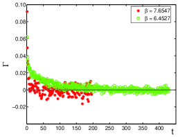
Refer to caption Refer to caption
Figure 7: Autocorrelation pattern of Zspin(2L)subscript𝑍spin2𝐿Z_{\rm spin}(2L) for two quenched simulations with L/a=16𝐿𝑎16L/a=16. Left: Normalized autocorrelation function plotted vs. the separation of measurements t𝑡t. Right: Integrated autocorrelation time τintsubscript𝜏int\tau_{\rm int} vs. the summation window WW{\rm W}. With β=7.6547𝛽7.6547\beta=7.6547 we have g¯2(L)=1.8811superscript¯𝑔2𝐿1.8811\bar{g}^{2}(L)=1.8811 (red asterisks), while for β=6.4527𝛽6.4527\beta=6.4527 we have g¯2(L)=3.480superscript¯𝑔2𝐿3.480\bar{g}^{2}(L)=3.480 (green circles). The vertical lines correspond to the optimal values of WW{\rm W} computed according to [?].
g¯2(L)superscript¯𝑔2𝐿\bar{g}^{2}(L) β𝛽\beta L/a𝐿𝑎L/a action F^μνsubscript^𝐹𝜇𝜈\hat{F}_{\mu\nu} ZspinSF(L)superscriptsubscript𝑍spinSF𝐿Z_{\rm spin}^{\rm SF}(L) ZspinSF(2L)superscriptsubscript𝑍spinSF2𝐿Z_{\rm spin}^{\rm SF}(2L) ΣspinsubscriptΣspin\Sigma_{\rm spin}
0.8873(5) 10.7503 6 1.3188(46) 1.3504(50) 1.0239(52)
0.8873(10) 11.0000 8 1.3218(22) 1.3532(51) 1.0238(42)
0.8873(30) 11.3384 12 1.3268(30) 1.3580(69) 1.0235(57)
0.9944(7) 10.0500 6 EH 1.3651(44) 1.3905(76) 1.0186(64)
0.9944(13) 10.3000 8 EH 1.3514(52) 1.3924(88) 1.0303(76)
0.9944(30) 10.6086 12 EH 1.3608(53) 1.384(12) 1.0171(96)
1.2430(13) 8.8997 6 1.4336(44) 1.4839(65) 1.0351(55)
1.2430(14) 9.1544 8 1.4278(30) 1.4803(56) 1.0367(45)
1.2430(35) 9.5202 12 1.4349(27) 1.474(10) 1.0275(74)
1.3293(12) 8.6129 6 EH 1.4727(57) 1.5116(77) 1.0264(66)
1.3293(21) 8.8500 8 EH 1.4664(71) 1.503(12) 1.0248(95)
1.3293(60) 9.1859 12 EH 1.4528(65) 1.517(13) 1.0438(99)
1.5553(15) 7.9993 6 1.5302(61) 1.6036(48) 1.0480(53)
1.5553(24) 8.2500 8 1.5229(46) 1.5999(78) 1.0506(60)
1.5553(70) 8.5985 12 1.5191(27) 1.579(11) 1.0394(77)
1.8811(22) 7.4082 6 1.6193(74) 1.7208(65) 1.0627(63)
1.8811(28) 7.6547 8 1.6100(55) 1.717(13) 1.0664(91)
1.8811(38) 7.9993 12 1.6015(42) 1.718(14) 1.0726(94)
2.1000(39) 7.1214 6 1.6563(87) 1.792(12) 1.0819(92)
2.1000(45) 7.3632 8 1.652(11) 1.773(11) 1.0732(96)
2.1000(80) 7.6985 12 1.6577(91) 1.751(17) 1.056(12)
2.4484(37) 6.7807 6 1.7618(88) 1.900(13) 1.0786(90)
2.4484(45) 7.0197 8 1.7371(86) 1.898(17) 1.092(11)
2.4484(80) 7.3551 12 1.7141(89) 1.855(17) 1.082(12)
2.770(7) 6.5512 6 1.8317(75) 2.085(19) 1.138(11)
2.770(7) 6.7860 8 1.8067(94) 2.044(17) 1.131(11)
2.770(11) 7.1190 12 1.7975(90) 2.000(23) 1.113(14)
2.770(7) 6.5512 6 HYP2 1.3659(36) 1.501(12) 1.0986(91)
2.770(7) 6.7860 8 HYP2 1.3643(24) 1.505(15) 1.103(11)
2.770(11) 7.1190 12 HYP2 1.3668(63) 1.490(14) 1.090(11)
3.480(8) 6.2204 6 HYP2 1.4329(53) 2.070(29) 1.444(21)
3.480(14) 6.4527 8 HYP2 1.4350(89) 1.975(31) 1.376(23)
3.480(39) 6.7750 12 HYP2 1.4465(61) 1.937(41) 1.339(29)
3.480(8) 6.257 6 1.9864(75) 2.714(32) 1.366(17)
3.480(8) 6.476 8 1.9492(75) 2.608(33) 1.338(18)
3.480(8) 6.257 6 HYP2 1.4297(47) 1.979(26) 1.384(19)
3.480(8) 6.476 8 HYP2 1.4262(29) 1.961(25) 1.375(17)
3.480(9) 6.799 12 HYP2 1.4280(33) 1.864(37) 1.305(26)
Table 5: Raw simulation results. The standard discretization is the HYP2 action of [?] and the clover leaf operator F^μνsubscript^𝐹𝜇𝜈\hat{F}_{\mu\nu}. Deviations from this rule are indicated. The improvement coefficient ctsubscript𝑐tc_{\rm t} is set to its 1-loop value, except for the last five lines, where 2-loop precision is used. The renormalized coupling is reproduced from [?].

As a check that the change of discretization does not introduce unwantedly large a2superscript𝑎2a^{2} effects, we also repeated the computation of σ(2.77)𝜎2.77\sigma(2.77) this way. Figure 2 nicely confirms the expected universality and a2superscript𝑎2a^{2} effects actually turn out to be reduced! We point out that with the Eichten-Hill action the cutoff effects can be directly compared to the expectations of perturbation theory. For the investigated couplings, g¯2=0.9944,1.3293superscript¯𝑔20.99441.3293\bar{g}^{2}=0.9944,1.3293, the agreement is very good.

The large amount of statistically independent measurements needed imposes strong limitations to the application of this method to the theory with dynamical fermions. The raw simulation results are reported in Table 5.

We finally add a remark on error estimates and autocorrelations in our simulations. The autocorrelation function ΓΓ\Gamma of Zspinsubscript𝑍spinZ_{\rm spin}, defined as in [?], falls very quickly for all our mesurements. At all but the largest coupling the integrated autocorrelation time is then easily estimated. However for L0.7fm𝐿0.7fmL\approx 0.7\,{\rm fm}, we observe that ΓΓ\Gamma shows a long tail before approaching zero. This pattern is absent in the smaller volumes, and shows little sensitivity to changes of NORsubscript𝑁ORN_{\rm OR}. Figure 7 (left) plots the ΓΓ\Gamma-function obtained from runs with (L/a,NUP,NOR)=(16,2,4)𝐿𝑎subscript𝑁UPsubscript𝑁OR1624(L/a,N_{\rm UP},N_{\rm OR})=(16,2,4), for two different physical volumes. Figure 7 (right) shows that for β=7.6547𝛽7.6547\beta=7.6547 the integrated autocorrelation time is quite short, i.e. τint=0.86(9)subscript𝜏int0.869\tau_{\rm int}=0.86(9), whereas for β=6.4527𝛽6.4527\beta=6.4527 the tail mentioned above leads to τint=2.15(13)subscript𝜏int2.1513\tau_{\rm int}=2.15(13). The latter translates into an increase of the error by a factor of two, in comparison to the case where no correlation is present (i.e. τint=0.5subscript𝜏int0.5\tau_{\rm int}=0.5).

References

  • [1] E. Eichten and B. Hill, An effective field theory for the calculation of matrix elements involving heavy quarks, Phys. Lett. B234 (1990) 511.
  • [2] B. Grinstein, The static quark effective theory, Nucl. Phys. B339 (1990) 253–268.
  • [3] H. Georgi, An effective field theory for heavy quarks at low energies, Phys. Lett. B240 (1990) 447–450.
  • [4] M. Bochicchio, G. Martinelli, C. R. Allton, C. T. Sachrajda, and D. B. Carpenter, Heavy quark spectroscopy on the lattice, Nucl. Phys. B372 (1992) 403–420.
  • [5] V. Gimenez, G. Martinelli, and C. T. Sachrajda, A high-statistics lattice calculation of λ1subscript𝜆1\lambda_{1} and λ2subscript𝜆2\lambda_{2} in the B-meson, Nucl. Phys. B486 (1997) 227–244, [hep-lat/9607055].
  • [6] JLQCD Collaboration, S. Aoki et. al., Heavy quark expansion parameters from lattice nrqcd, Phys. Rev. D69 (2004) 094512, [hep-lat/0305024].
  • [7] E. Eichten and B. Hill, Static effective field theory: 1/m1𝑚1/m corrections, Phys. Lett. B243 (1990) 427–431.
  • [8] J. M. Flynn and B. R. Hill, B - B splitting: A test of heavy quark methods, Phys. Lett. B264 (1991) 173–177.
  • [9] M. Lüscher, P. Weisz, and U. Wolff, A numerical method to compute the running coupling in asymptotically free theories, Nucl. Phys. B359 (1991) 221–243.
  • [10] ALPHA Collaboration, A. Bode et. al., First results on the running coupling in QCD with two massless flavors, Phys. Lett. B515 (2001) 49–56, [hep-lat/0105003].
  • [11] ALPHA Collaboration, S. Capitani, M. Lüscher, R. Sommer, and H. Wittig, Non-perturbative quark mass renormalization in quenched lattice QCD, Nucl. Phys. B544 (1999) 669, [hep-lat/9810063].
  • [12] ALPHA Collaboration, J. Heitger and R. Sommer, Non-perturbative heavy quark effective theory, JHEP 02 (2004) 022, [hep-lat/0310035].
  • [13] M. Della Morte, N. Garron, M. Papinutto, and R. Sommer, Heavy quark effective theory computation of the mass of the bottom quark, JHEP 01 (2007) 007, [hep-ph/0609294].
  • [14] J. H. Kuhn, M. Steinhauser, and C. Sturm, Heavy quark masses from sum rules in four-loop approximation, hep-ph/0702103.
  • [15] ALPHA Collaboration, J. Rolf and S. Sint, A precise determination of the charm quark’s mass in quenched QCD, JHEP 12 (2002) 007, [hep-ph/0209255].
  • [16] D. Guazzini, R. Sommer, and N. Tantalo, mbsubscript𝑚𝑏m_{b} and fBssubscript𝑓subscript𝐵𝑠f_{B_{s}} from a combination of hqet and qcd, PoS LAT2006 (2006) 084, [hep-lat/0609065].
  • [17] ALPHA Collaboration, M. Kurth and R. Sommer, Renormalization and O(a𝑎a)-improvement of the static axial current, Nucl. Phys. B597 (2001) 488–518, [hep-lat/0007002].
  • [18] M. Della Morte, A. Shindler, and R. Sommer, On lattice actions for static quarks, JHEP 08 (2005) 051, [hep-lat/0506008].
  • [19] ALPHA Collaboration, M. Della Morte et. al., Lattice hqet with exponentially improved statistical precision, Phys. Lett. B581 (2004) 93–98, [hep-lat/0307021].
  • [20] M. Lüscher, S. Sint, R. Sommer, and P. Weisz, Chiral symmetry and O(a𝑎a) improvement in lattice QCD, Nucl. Phys. B478 (1996) 365–400, [hep-lat/9605038].
  • [21] ALPHA Collaboration, J. Heitger, A. Jüttner, R. Sommer, and J. Wennekers, Non-perturbative tests of heavy quark effective theory, JHEP 11 (2004) 048, [hep-ph/0407227].
  • [22] R. Sommer, Non-perturbative qcd: Renormalization, o(a)𝑎(a)-improvement and matching to heavy quark effective theory, hep-lat/0611020.
  • [23] A. F. Falk, B. Grinstein, and M. E. Luke, Leading mass corrections to the heavy quark effective theory, Nucl. Phys. B357 (1991) 185–207.
  • [24] G. Amoros, M. Beneke, and M. Neubert, Two-loop anomalous dimension of the chromo-magnetic moment of a heavy quark, Phys. Lett. B401 (1997) 81–90, [hep-ph/9701375].
  • [25] A. Czarnecki and A. G. Grozin, Hqet chromomagnetic interaction at two loops, Phys. Lett. B405 (1997) 142–149, [hep-ph/9701415].
  • [26] A. Grozin, P. Marquard, J. Piclum, and M. Steinhauser SFB/TR 09, to be published.
  • [27] M. Lüscher, R. Sommer, P. Weisz, and U. Wolff, A precise determination of the running coupling in the SU(3) Yang-Mills theory, Nucl. Phys. B413 (1994) 481–502, [hep-lat/9309005].
  • [28] E. Eichten and F. Feinberg, Spin dependent forces in qcd, Phys. Rev. D23 (1981) 2724.
  • [29] D. Gromes, Spin dependent potentials in qcd and the correct long range spin orbit term, Z. Phys. C26 (1984) 401.
  • [30] N. Brambilla, A. Pineda, J. Soto, and A. Vairo, Effective field theories for heavy quarkonium, hep-ph/0410047.
  • [31] Y. Koma and M. Koma, Spin-dependent potentials from lattice qcd, hep-lat/0609078.
  • [32] E. Eichten and B. Hill, Renormalization of heavy - light bilinears and fbsubscript𝑓𝑏f_{b} for Wilson fermions, Phys. Lett. B240 (1990) 193.
  • [33] M. Della Morte, R. Hoffmann, and F. Knechtli, Discrete symmetries of lattice qcd (and the sf), Internal notes of the ALPHA Collaboration (2005).
  • [34] S. Sint and R. Sommer, The running coupling from the QCD Schrödinger functional: A one loop analysis, Nucl. Phys. B465 (1996) 71–98, [hep-lat/9508012].
  • [35] ALPHA Collaboration, S. Sint and P. Weisz, The running quark mass in the sf scheme and its two loop anomalous dimension, Nucl. Phys. B545 (1999) 529, [hep-lat/9808013].
  • [36] ALPHA Collaboration, M. Della Morte et. al., Non-perturbative quark mass renormalization in two-flavor qcd, Nucl. Phys. B729 (2005) 117–134, [hep-lat/0507035].
  • [37] ALPHA Collaboration, M. Guagnelli, R. Sommer, and H. Wittig, Precision computation of a low-energy reference scale in quenched lattice QCD, Nucl. Phys. B535 (1998) 389, [hep-lat/9806005].
  • [38] A. Huntley and C. Michael, Spin spin and spin - orbit potentials from lattice gauge theory, Nucl. Phys. B286 (1987) 211.
  • [39] ALPHA Collaboration, M. Guagnelli, J. Heitger, C. Pena, S. Sint, and A. Vladikas, Non-perturbative renormalization of left-left four-fermion operators in quenched lattice qcd, JHEP 03 (2006) 088, [hep-lat/0505002].
  • [40] F. Palombi, C. Pena, and S. Sint, A perturbative study of two four-quark operators in finite volume renormalization schemes, JHEP 03 (2006) 089, [hep-lat/0505003].
  • [41] F. Palombi, M. Papinutto, C. Pena, and H. Wittig, A strategy for implementing non-perturbative renormalisation of heavy-light four-quark operators in the static approximation, JHEP 08 (2006) 017, [hep-lat/0604014].
  • [42] C. Pena, Twisted mass qcd for weak matrix elements, PoS LAT2006 (2006) 019, [hep-lat/0610109].
  • [43] ALPHA Collaboration, J. Heitger, M. Kurth, and R. Sommer, Non-perturbative renormalization of the static axial current in quenched qcd, Nucl. Phys. B669 (2003) 173–206, [hep-lat/0302019].
  • [44] M. Della Morte, P. Fritzsch, and J. Heitger, Non-perturbative renormalization of the static axial current in two-flavour qcd, JHEP 02 (2007) 079, [hep-lat/0611036].
  • [45] S. Kurth, The renormalised quark mass in the Schrödinger functional of lattice QCD: A one-loop calculation with a non- vanishing background field, hep-lat/0211011.
  • [46] R. Narayanan and U. Wolff, Two loop computation of a running coupling in lattice yang- mills theory, Nucl. Phys. B444 (1995) 425–446, [hep-lat/9502021].
  • [47] ALPHA Collaboration, A. Bode, P. Weisz, and U. Wolff, Two loop computation of the Schrödinger functional in lattice QCD, Nucl. Phys. B576 (2000) 517–539, [Erratum-ibid.B600:453,2001, Erratum-ibid.B608:481,2001, hep-lat/9911018].
  • [48] P. Weisz, Computation of the improvement coefficient cswsubscript𝑐𝑠𝑤c_{sw} to 1-loop, Internal notes of the ALPHA Collaboration (1996).
  • [49] M. Creutz, Quarks, gluons and lattices, . Cambridge, Uk: Univ. Pr. ( 1983) 169 P. ( Cambridge Monographs On Mathematical Physics).
  • [50] G. M. de Divitiis, R. Frezzotti, M. Guagnelli, and R. Petronzio, Nonperturbative determination of the running coupling constant in quenched su(2), Nucl. Phys. B433 (1995) 390–402, [hep-lat/9407028].
  • [51] N. Cabibbo and E. Marinari, A new method for updating su(n) matrices in computer simulations of gauge theories, Phys. Lett. B119 (1982) 387–390.
  • [52] K. Fabricius and O. Haan, Heat bath method for the twisted eguchi-kawai model, Phys. Lett. B143 (1984) 459.
  • [53] A. D. Kennedy and B. J. Pendleton, Improved heat bath method for monte carlo calculations in lattice gauge theories, Phys. Lett. B156 (1985) 393–399.
  • [54] M. Creutz, Overrelaxation and monte carlo simulation, Phys. Rev. D36 (1987) 515.
  • [55] G. Parisi, R. Petronzio, and F. Rapuano, A measurement of the string tension near the continuum limit, Phys. Lett. 128B (1983) 418.
  • [56] M. Lüscher and P. Weisz, Locality and exponential error reduction in numerical lattice gauge theory, JHEP 09 (2001) 010, [hep-lat/0108014].
  • [57] ALPHA Collaboration, U. Wolff, Monte carlo errors with less errors, Comput. Phys. Commun. 156 (2004) 143–153, [hep-lat/0306017].