A case for variational geomagnetic data assimilation: insights from a one-dimensional, nonlinear, and sparsely observed MHD system 111Article published in Nonlinear Processes in Geophysics, 14, 163–180, 2007. The paper can be freely downloaded from the journal webpage http://www.copernicus.org/EGU/npg/npg.html
Abstract
Secular variations of the geomagnetic field have been measured with a continuously improving accuracy during the last few hundred years, culminating nowadays with satellite data. It is however well known that the dynamics of the magnetic field is linked to that of the velocity field in the core and any attempt to model secular variations will involve a coupled dynamical system for magnetic field and core velocity. Unfortunately, there is no direct observation of the velocity. Independently of the exact nature of the above-mentioned coupled system – some version being currently under construction – the question is debated in this paper whether good knowledge of the magnetic field can be translated into good knowledge of core dynamics. Furthermore, what will be the impact of the most recent and precise geomagnetic data on our knowledge of the geomagnetic field of the past and future? These questions are cast into the language of variational data assimilation, while the dynamical system considered in this paper consists in a set of two oversimplified one-dimensional equations for magnetic and velocity fields. This toy model retains important features inherited from the induction and Navier-Stokes equations: non-linear magnetic and momentum terms are present and its linear response to small disturbances contains Alfvén waves. It is concluded that variational data assimilation is indeed appropriate in principle, even though the velocity field remains hidden at all times; it allows us to recover the entire evolution of both fields from partial and irregularly distributed information on the magnetic field. This work constitutes a first step on the way toward the reassimilation of historical geomagnetic data and geomagnetic forecast.
1 Introduction
The magnetic observation of the earth with satellites has now matured to a point where continuous measurements of the field are available from 1999 onwards, thanks to the Oersted, SAC-C, and CHAMP missions (e.g. Olsen et al., 2000; Maus et al., 2005, and references therein). In conjunction with ground-based measurements, such data have been used to produce a main field model of remarkable accuracy, in particular concerning the geomagnetic secular variation (GSV)(Olsen et al., 2006a). Let us stress that we are concerned in this paper with recent changes in the earth’s magnetic field, occurring over time scales on the order of decades to centuries. This time scale is nothing compared to the age of the earth’s dynamo ( Gyr), or the average period at which the dynamo reverses its polarity (a few hundreds of kyr, see for instance Merrill et al. (1996)), or even the magnetic diffusion time scale in earth’s core, on the order of kyr (e.g. Backus et al., 1996). It is, however, over this minuscule time window that the magnetic field and its changes are by far best documented (e.g. Bloxham et al., 1989).
Downward-projecting the surface magnetic field at the core-mantle boundary, and applying the continuity of the normal component of the field across this boundary, one obtains a map of this particular component at the top of the core. The catalog of these maps at different epochs constitutes most of the data we have at hand to estimate the core state. Until now, this data has been exploited within a kinematic framework (Roberts and Scott, 1965; Backus, 1968): the normal component of the magnetic field is a passive tracer, the variations of which are used to infer the velocity that transports it (e.g. Le Mouël, 1984; Bloxham, 1989). For the purpose of modeling the core field and interpreting its temporal variations not only in terms of core kinematics, but more importantly in terms of core dynamics, it is crucial to make the best use of the new wealth of satellite data that will become available to the geomagnetic community, especially with the launch of the SWARM mission around 2010 (Olsen et al., 2006b).
This best use can be achieved in the framework of data assimilation. In this respect, geomagnetists are facing challenges similar to the ones oceanographers were dealing with in the early Nineteen-nineties, with the advent of operational satellite observation of the oceans. Inasmuch as oceanographers benefited from the pioneering work of their atmosphericist colleagues (data assimilation is routinely used to improve weather forecasts), geomagnetists must rely on the developments achieved by the oceanic and atmospheric communities to assemble the first bricks of geomagnetic data assimilation. Dynamically speaking, the earth’s core is closer to the oceans than to the atmosphere. The similarity is limited though, since the core is a conducting fluid whose dynamics are affected by the interaction of the velocity field with the magnetic field it sustains. These considerations, and their implications concerning the applicability of sophisticated ocean data assimilation strategies to the earth’s core, will have to be addressed in the future. Today, geomagnetic data assimilation is still in its infancy (see below for a review of the efforts pursued in the past couple of years). We thus have to ask ourselves zero-th order questions, such as: variational or sequential assimilation?
In short, one might be naively tempted to say that variational data assimilation (VDA) is more versatile than sequential data assimilation (SDA), at the expense of a more involved implementation -for an enlightening introduction to the topic, see Talagrand (1997). Through an appropriately defined misfit function, VDA can in principle answer any question of interest, provided that one resorts to the appropriate adjoint model. In this paper, we specifically address the issue of improving initial conditions to better explain a data record, and show how this can be achieved, working with a non-linear, one-dimensional magneto-hydrodynamic (MHD) model. SDA is more practical, specifically geared towards better forecasts of the model state, for example in numerical weather prediction (Talagrand, 1997). No adjoint model is needed here; the main difficulty lies in the computational burden of propagating the error covariance matrix needed to perform the so-called analysis, the operation by which past information is taken into account in order to better forecast future model states (e.g. Brasseur, 2006).
Promising efforts in applying SDA concepts and techniques to geomagnetism have recently been pursued: Liu et al. (2007) have performed so-called Observing System Simulation Experiments (OSSEs) using a three-dimensional model of the geodynamo, to study in particular the response (as a function of depth) of the core to surface measurements of the normal component of the magnetic field, for different approximations of the above mentioned error covariance matrix. Also, in the context of a simplified one-dimensional MHD model, which retains part of the ingredients that make the complexity (and the beauty) of the geodynamo, Sun et al. (2007) have applied an optimal interpolation scheme that uses a Monte-Carlo method to calculate the same matrix, and studied the response of the system to assimilation for different temporal and spatial sampling frequencies. Both studies show a positive response of the system to SDA (i.e. better forecasts).
In our opinion, though, SDA is strongly penalized by its formal impossibility to use current observations to improve past data records -even if this does not hamper its potential to produce good estimates of future core states. As said above, most of the information we have about the core is less that yr old (Jackson et al., 2000). This record contains the signatures of the phenomena responsible for its short-term dynamics, possibly hydromagnetic waves with periods of several tens of years (Finlay and Jackson, 2003). Our goal is to explore the VDA route in order to see to which extent high-resolution satellite measurements of the earth’s magnetic field can help improve the historical magnetic database, and identify more precisely physical phenomena responsible for short-term geomagnetic variations. To tackle this problem, we need a dynamical model of the high-frequency dynamics of the core, and an assimilation strategy. The aim of this paper is to reveal the latter, and illustrate it with a simplified one-dimensional nonlinear MHD model. Such a toy model, similar to the one used by Sun et al. (2007), retains part of the physics, at the benefit of a negligible computational cost. It enables intensive testing of the assimilation algorithm.
This paper is organized as follows: the methodology we shall pursue in applying variational data assimilation to the geomagnetic secular variation is presented in Sect. 2; its implementation for the one-dimensional, nonlinear MHD toy model is described in detail in Sect. 3. Various synthetic assimilation experiments are presented in Sect. 4, the results of which are summarized and further discussed in Sect. 5.
2 Methodology
In this section, we outline the bases of variational geomagnetic data assimilation, with the mid-term intent of improving the quality of the past geomagnetic record using the high-resolution information recorded by satellites. We resort to the unified set of notations proposed by Ide et al. (1997). What follows is essentially a transcription of the landmark paper by Talagrand and Courtier (1987) with these conventions, transcription to which we add the possibility of imposing constraints to the core state itself during the assimilation process.
2.1 Forward model
Assume we have a prognostic, nonlinear, numerical model which describes the dynamical evolution of the core state at any discrete time . If denotes the time-step size, the width of the time window considered here is , the initial (final) time being (). In formal assimilation parlance, this is written as
| (1) |
in which is a column vector describing the model state. If relies for instance on the discretization of the equations governing secular variation with a grid-based approach, this vector contains the values of all the field variables at every grid point. The secular variation equations could involve terms with a known, explicit time dependence, hence the dependence of on time in Eq. (1). Within this framework, the modeled secular variation is entirely controlled by the initial state of the core, .
2.2 Observations
Assume now that we have knowledge of the true dynamical state of the core through databases of observations collected at discrete locations in space and time:
| (2) |
in which and are the discrete observation operator and noise, respectively. For GSV, observations consist of (scalar or vector) measurements of the magnetic field, possibly supplemented by decadal timeseries of the length of day, since these are related to the angular momentum of the core (Jault et al., 1988; Bloxham, 1998). The observation operator is assumed linear and time-dependent: in the context of geomagnetic data assimilation, we can safely anticipate that its dimension will increase dramatically when entering the recent satellite era (1999-present). However, will always produce vectors whose dimension is much lower than the dimension of the state itself: this fundamental problem of undersampling is at the heart of the development of data assimilation strategies. The observational error is time-dependent as well: it is assumed to have zero mean and we denote its covariance matrix at discrete time by .
2.3 Quadratic misfit functions
Variational assimilation aims here at improving the definition of the initial state of the core to produce modeled observations as close as possible to the observations of the true state. The distance between observations and predictions is measured using a quadratic misfit function
| (3) |
in which the superscript ‘’ means transpose. In addition to the distance between observations and predictions of the past record, we might as well wish to try and apply some further constraints on the core state that we seek, through the addition of an extra cost function
| (4) |
in which is a matrix which describes the constraint one would like to be subject to. This constraint can originate from some a priori ideas about the physics of the true state of the system, and its implication on the state itself, should this physics not be properly accounted for by the model , most likely because of its computational cost. In the context of geomagnetic data assimilation, this a priori constraint can come for example from the assumption that fluid motions inside the rapidly rotating core are almost invariant along the direction of earth’s rotation, according to Taylor–Proudman’s theorem (e.g. Greenspan, 1990). We shall provide the reader with an example for when applying these theoretical concepts to the 1D MHD model (see Sect. 4.2).
Consequently, we write the total misfit function as
| (5) |
where and are the weights of the observational and constraint-based misfits, respectively. These two coefficients should be normalized; we will discuss the normalization in Sect. 4.
2.4 Sensitivity to the initial conditions
To minimize , we express its sensitivity to , namely . With our conventions, is a row vector, since a change in , , is responsible for a change in , , given by
| (6) |
To compute this gradient, we first introduce the tangent linear operator which relates a change in to a change in the core state at the preceding discrete time, :
| (7) |
The tangent linear operator is obtained by linearizing the model about the state . Successive applications of the above relationship allow us to relate perturbations of the state vector at a given model time to perturbations of the initial state :
| (8) |
The sensitivity of to any expresses itself via
| (9) |
that is
| (10) |
Additionally, after differentiating Eq. (5) using Eqs. (3) and (4), we obtain
Gathering the observational and constraint contributions to originating from every state vector finally yields
which implies in turn that
| (11) | |||||
2.5 The adjoint model
The computation of via Eq. (11) is injected in an iterative method to adjust the initial state of the system to try and minimize . The -th step of this algorithm is given in general terms by
| (12) |
in which is a descent direction, and an appropriate chosen scalar. In the case of the steepest descent algorithm, , and is an a priori set constant. The descent direction is a column vector, hence the need to take the transpose of . In practice, the transpose of Eq. (11) yields, at the -th step of the algorithm,
| (13) | |||||
Introducing the adjoint variable , the calculation of is therefore performed practically by integrating the so-called adjoint model
| (14) |
starting from , and going backwards in order to finally estimate
| (15) |
Equation (14) is at the heart of variational data assimilation (Talagrand, 1997). Some remarks and comments concerning this so-called adjoint equation are in order:
-
1.
It requires to implement the transpose of the tangent linear operator, the so-called adjoint operator, . If the discretized forward model is cast in terms of matrix-matrix and/or matrix-vector products, then this implementation can be rather straightforward (see Sect. 3). Still, for realistic applications, deriving the discrete adjoint equation can be rather convoluted (e.g. Bennett, 2002, Chap. 4).
-
2.
The discrete adjoint equation (Eq. 14) is based on the already discretized model of the secular variation. Such an approach is essentially motivated by practical reasons, assuming that we already have a numerical model of the geomagnetic secular variation at hand. We should mention here that a similar effort can be performed at the continuous level, before discretization. The misfit can be defined at this level; the calculus of its variations gives then rise to the Euler–Lagrange equations, one of which being the continuous backward, or adjoint, equation. One could then simply discretize this equation, using the same numerical approach as the one used for the forward model, and use this tool to adjust . According to Bennett (2002), though, the “discrete adjoint equation” is not the “adjoint discrete equation”, the former breaking adjoint symmetry, which results in a solution being suboptimal (Bennett, 2002, § 4.1.6).
-
3.
Aside from the initial state , one can in principle add model parameters (, say) as adjustable variables, and invert jointly for and , at the expense of expressing the discrete sensitivity of to as well. For geomagnetic VDA, this versatility might be of interest, in order for instance to assess the importance of magnetic diffusion over the time window of the historical geomagnetic record.
-
4.
The whole sequence of core states , has to be kept in memory. This memory requirement can become quite significant when considering dynamical models of the GSV. Besides, even if the computational cost of the adjoint model is by construction equivalent to the cost of the forward model, the variational assimilation algorithm presented here is at least one or two orders of magnitude more expensive than a single forward realization, because of the number of iterations needed to obtain a significant reduction of the misfit function. When tackling ‘real’ problems in the future (as opposed to the illustrative problem of the next sections), memory and CPU time constraints might make it necessary to lower the resolution of the forward (and adjoint) models, by taking parameters values further away from the real core. A constraint such as the one imposed through Eq. (4) can then appear as a way to ease the pain and not to sacrifice too much physics, at negligible extra computational cost.
We give a practical illustration of these ideas and concepts in the next two sections.
3 Application to a one-dimensional nonlinear MHD model
We consider a conducting fluid, whose state is fully characterized by two scalar fields, and . Formally, represents the magnetic field (it can be observed), and is the velocity field (it is invisible).
3.1 The forward model
3.1.1 Governing equations
The conducting fluid has density , kinematic viscosity , electrical conductivity , magnetic diffusivity , and magnetic permeability (). Its pseudo-velocity and pseudo-magnetic field are both scalar fields, defined over a domain of length , . We refer to pseudo fields here since these fields are not divergence-free. If they were so, they would have to be constant over the domain, which would considerably limit their interest from the assimilation standpoint. Bearing this remark in mind, we shall omit the ‘pseudo’ adjective in the remainder of this study.
We choose as the length scale, the magnetic diffusion time scale as the time scale, as the magnetic field scale, and as the velocity scale (i.e. the Alfvén wave speed). Accordingly, the evolution of and is controlled by the following set of non-dimensional equations:
| (16) | |||||
| (17) |
supplemented by the boundary and initial conditions
| (18) | |||||
| (19) | |||||
| (20) |
Eq. (16) is the momentum equation: the rate of change of the velocity is controlled by advection, magnetic forces and diffusion. Similarly, in the induction equation (17), the rate of change of the magnetic field results from the competition between inductive effects and ohmic diffusion.
Two non-dimensional numbers define this system,
which is the Lundquist number (ratio of the magnetic diffusion time scale to the Alfvén time scale), and
which is the magnetic Prandtl number, a material property very small for liquid metals - for earth’s core (e.g. Poirier, 1988).
3.1.2 Numerical model
Fields are discretized in space using one Legendre spectral element of order . In such a framework, basis functions are the Lagrangian interpolants defined over the collection of Gauss–Lobatto–Legendre (GLL) points (for a comprehensive description of the spectral element method, see Deville et al., 2002). Figure 1 shows such a basis function for . Having basis functions defined everywhere over makes it straightforward to define numerically the observation operator (see Sect. 3.3). We now drop the superscript for the sake of brevity. The semi-discretized velocity and magnetic fields are column vectors, denoted with bold fonts
| (21) | |||||
| (22) |

Discretization is performed in time with a semi-implicit finite-differencing scheme of order , explicit for nonlinear terms, and implicit for diffusive terms. As in the previous section, assuming that is the time step size, we define As a result of discretization in both space and time, the model is advanced in time by solving the following algebraic system
| (23) |
where
| (24) | |||||
| (25) | |||||
| (26) | |||||
| (27) |
are the Helmholtz operators acting on velocity field and the magnetic field, and the forcing terms for each of these two, respectively. We have introduced the following definitions :
-
•
, which is the diagonal mass matrix,
-
•
, which is the so-called stiffness matrix (it is symmetric definite positive),
-
•
, which denotes the Hadamard product: ,
-
•
and , the so-called derivative matrix
(28)
the knowledge of which is required to evaluate the nonlinear terms. Advancing in time requires to invert both Helmholtz operators, which we do directly resorting to standard linear algebra routines (Anderson et al., 1999). Let us also bear in mind that the Helmholtz operators are symmetric (i.e. self-adjoint).
In assimilation parlance, and according to the conventions introduced in the previous section, the state vector is consequently equal to , and its dimension is (since the value of both the velocity and magnetic fields are prescribed on the boundaries of the domain).
3.2 The true state
Since we are dealing in this paper with synthetic observations, it is necessary to define the true state of the 1D system as the state obtained via the integration of the numerical model defined in the preceding paragraph, for a given set of initial conditions, and specific values of the Lundquist and magnetic Prandtl numbers, and . The true state (denoted with the superscript ‘’) will always refer to the following initial conditions
| (29) | |||||
| (30) |
along with and . The model is integrated forward in time until (a fifth of a magnetic diffusion time). The polynomial order used to compute the true state is , and the time step size . Figure 2 shows the velocity (left) and magnetic field (right) at initial (black curves) and final (red curves) model times.
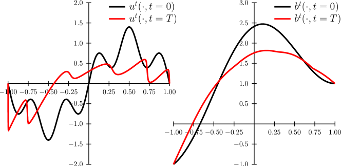
The low value of the magnetic Prandtl number reflects itself in the sharp velocity boundary layers that develop near the domain boundaries, while the magnetic field exhibits in contrast a smooth profile (the magnetic diffusivity being three orders of magnitude larger than the kinematic viscosity). To properly resolve these Hartmann boundary layers there must be enough points in the vicinity of the domain boundaries: we benefit here from the clustering of GLL points near the boundaries (Deville et al., 2002). Besides, even if the magnetic profile is very smooth, one can nevertheless point out here and there kinks in the final profile. These kinks are associated with sharp velocity gradients (such as the one around ) and are a consequence of the nonlinear term in the induction Eq. (17).
3.3 Observation of the true state
In order to mimic the situation relevant for the earth’s core and geomagnetic secular variation, assume that we have knowledge of at discrete locations in space and time, and that the velocity is not measurable. For the sake of generality, observations of are not necessarily made at collocation points, hence the need to define a spatial observation operator (at discrete time ) consistent with the numerical approximation introduced above. If denotes the number of virtual magnetic stations at time , and their locations (), is a rectangular matrix, whose coefficients write
| (31) |
A database of magnetic observations is therefore produced at discrete time via the matrix-vector product
| (32) |
Integration of the adjoint model also requires the knowledge of the transpose of the observation operator (Eq. 14), the construction of which is straightforward according to the previous definition. To construct the set of synthetic observations, we take for simplicity the observational noise to be zero. During the assimilation process, we shall assume that estimation errors are uncorrelated, and that the level of confidence is the same for each virtual observatory. Consequently,
| (33) |
in which is the identity matrix, throughout the numerical experiments.
As an aside, let us notice that magnetic observations could equivalently consist of an (arbitrarily truncated) set of spectral coefficients, resulting from the expansion of the magnetic field on the basis of Legendre polynomials. Our use of stations is essentially motivated by the fact that our forward model is built in physical space. For real applications, a spectral approach is interesting since it can naturally account for the potential character of the field in a source-free region; however, it is less amenable to the spatial description of observation errors, if these do not vary smoothly.
3.4 The adjoint model
3.4.1 The tangent linear operator
As stated in the the previous section, the tangent linear operator at discrete time is obtained at the discrete level by linearizing the model about the current solution . By perturbing these two fields
| (34) | |||
| (35) |
we get (after some algebra)
having introduced the following matrices
| (36) | |||||
| (37) | |||||
| (38) | |||||
| (39) |
Aside from the identity matrix , matrices and notations appearing in these definitions have already been introduced in §3.1.2. In connection with the general definition introduced in the previous section, , is the block matrix
| (40) |
3.4.2 Implementation of the adjoint equation
The sensitivity of the model to its initial conditions is computed by applying the adjoint operator, , to the adjoint variables - see Eq. (14). According to Eq. (40), one gets
| (41) |
with each transpose given by
| (42) | |||||
| (43) | |||||
| (44) | |||||
| (45) |
In writing the equation in this form, we have used the symmetry properties of the Helmholtz and mass matrices, and introduced the transpose of the derivative matrix, . Programming the adjoint model is very similar to programming the forward model, provided that one has cast the latter in terms of matrix-matrix, matrix-vector, and Hadamard products.
4 Synthetic assimilation experiments
Having all the numerical tools at hand, we start out by assuming that we have imperfect knowledge of the initial model state, through an initial guess , with the model parameters and resolution equal to the ones that helped us define the true state of §3.2. We wish here to quantify how assimilation of observations can help improve the knowledge of the initial (and subsequent) states, with particular emphasis on the influence of spatial and temporal sampling. In the series of results reported in this paragraph, the initial guess at model initial time is :
| (46) | |||||
| (47) |
With respect to the true state at the initial time, the first guess is missing the small-scale component of , i.e. the second term on the right-hand side of Eq. (29). In addition, our estimate of has an extra parasitic large-scale component (the third term on the right-hand side of Eq. (47)), a situation that could occur when dealing with the GSV, for which the importance of unmodeled small-scale features has been recently put forward given the accuracy of satellite data (Eymin and Hulot, 2005). Figure 3 shows the initial and final and , along with and at the same epochs for comparison, and the difference between the two, multiplied by a factor of five.
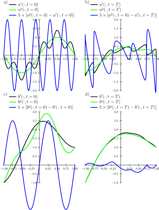
Differences in are not pronounced. Over the time window considered here, the parasitic small-scale component has undergone considerable diffusion. To quantify the differences between the true state and the guess, we resort to the norm
and define the relative magnetic and fluid errors at time by
| (48) | |||||
| (49) |
The initial guess given by Eqs. (46)(47) is characterized by the following errors: and .
4.1 Improvement of the initial guess with no a priori constraint on the state
4.1.1 Regular space and time sampling
Observations of are performed at virtual observatories which are equidistant in space, at a number of epochs evenly distributed over the time interval. Assuming no a priori constraint on the state, we set in Def. 5. The other constant
The minimization problem is tackled by means of a conjugate gradient algorithm, à la Polak–Ribière (Shewchuk, 1994). Iterations are stopped either when the initial misfit has decreased by 8 orders of magnitude, or when the iteration count exceeds 5,000. In most cases, the latter situation has appeared in our simulations. A typical minimization is characterized by a fast decrease in the misfit during the first few tens of iterations, followed by a slowly decreasing (almost flat) behaviour. Even if the solution keeps on getting better (i.e. closer to the synthetic reality) during this slow convergence period, practical considerations (having in mind the cost of future geomagnetic assimilations) prompted us to stop the minimization.
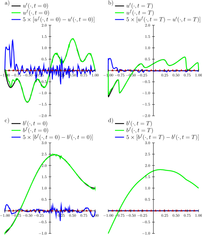
A typical example of a variational assimilation result is shown in Fig. 4. In this case, and . The recovery of the final magnetic field is excellent (see Fig. 4d), the relative error being . The benefit here is double: first, the network of observatories is dense enough to sample properly the field, and second, a measurement is made exactly at this discrete time instant, leaving no time for error fields to develop. When the latter is possible, the recovered fields can be contaminated by small-scale features, that is features that have length scales smaller than the spatial sampling scale. We see this happening in Fig. 4c), in which the magnified difference between the recovered and true , shown in blue, appears indeed quite spiky; has still decreased from an initial value of (Fig. 3c) down to . Results for velocity are shown in Figs. 4a and 4b. The recovered velocity is closer to the true state than the initial guess: this is the expected benefit from the nonlinear coupling between velocity and magnetic field in Eqs. (16)-(17). The indirect knowledge we have of , through the observation of , is sufficient to get better estimates of this field variable. At the end of the assimilation process, and , which were approximately equal to with the initial guess, have been brought down to and %, respectively. The velocity at present time (Fig. 4) is remarkably close to the true velocity, save for the left boundary layer sharp structure, which is undersampled (see the distribution of red triangles).
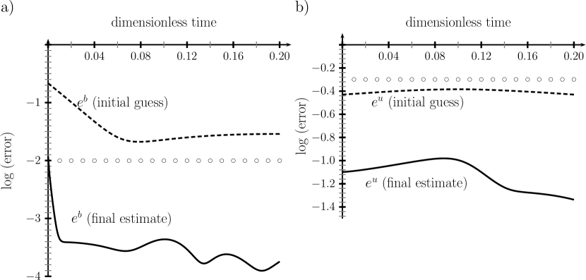
We further document the dynamical evolution of errors by plotting on Fig. 5 the temporal evolution of and for this particular configuration. Instants at which observations are made are represented by circles, and the temporal evolution of the guess errors are also shown for comparison. The guess for the initial magnetic field is characterized by a decrease of the error that occurs over diffusion time scale, that is roughly the time it takes for most of the parasitic small-scale error component to diffuse away, the error being then dominated at later epochs by advection errors, originating from errors in the velocity field. The recovered magnetic field (Fig. 5a, solid line), is in very good agreement with the true field as soon as measurements are available ( of a magnetic diffusion time, see the circles on Fig. 5a). Even though no measurements are available for the initial epoch, the initial field has also been corrected significantly, as discussed above. In the latter parts of the record, oscillations in the magnetic error field are present -they disappear if the minimization is pushed further (not shown).
The unobserved velocity field does not exhibit such a drastic reduction in error as soon as observations are available (Fig. 5b, solid line). Still, it is worth noticing that the velocity error is significantly smaller in the second part of the record, in connection with the physical observation that most of the parasitic small-scale component of the field has decayed away (see above): advection errors dominate in determining the time derivative of in Eq. (17), leaving room for a better assessment of the value of . For other cases (different and ), we find a similar behaviour (not shown). We comment on the effects of an irregular time sampling on the above observations in section 4.1.3.
Having in mind what one gets in this particular configuration, we now summarize in Fig. 6 results obtained by varying systematically these parameters. After assimilation, the logarithmic value of the velocity and magnetic field errors, at the initial and final stages ( and ), are plotted versus , using and virtual magnetic stations. As far as temporal sampling is concerned, can be equal to (having one observation at present time only), , , or .
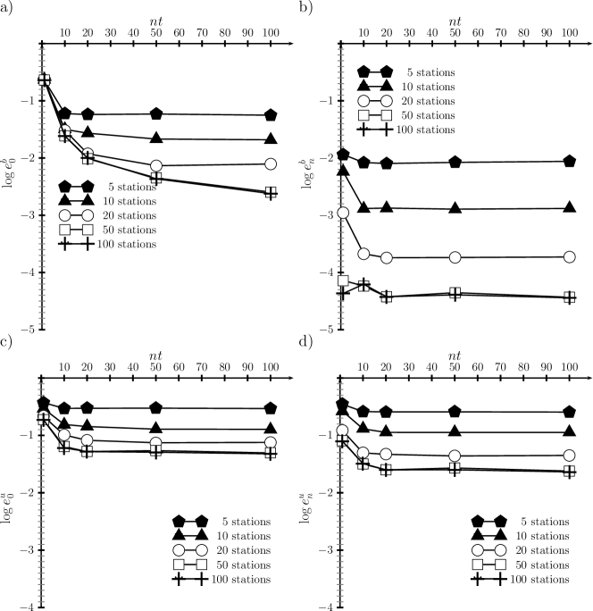
Inspection of Fig. 6 leads us to make the following comments:
-
•
Regarding :
-
–
50 stations are enough to properly sample the magnetic field in space. In this case is sufficient to properly determine , and no real improvement is made when increasing (Fig. 6b). During the iterative process, the value of the field is brought to its observed value at every station of the dense network, and this is it: no dynamical information is needed.
-
–
When, on the other hand, spatial sampling is not good enough, information on the dynamics of helps improve partially its knowledge at present time. For instance, we get a factor of reduction in with , going from to (Fig. 6b, circles). The improvement then stabilizes upon increasing : spatial error dominates.
-
–
This also applies for the initial magnetic field , see Fig. 6a. As a matter of fact, having no dynamical information about () precludes any improvement on , for any density of the spatial network. Improvement occurs for . If the spatial coverage is good enough (), no plateau is reached, since the agreement between the assimilated and true fields keeps on getting better, as it should.
-
–
-
•
Regarding :
- –
-
–
If is increased, the error decreases and reaches a plateau which is again determined by spatial resolution. This holds for and . For the reason stated above, is better known than . The error is dominated in both cases by a poor description of the left boundary layer (see the blue curves in Figs. 4a and 4b). The gradient associated with this layer is not sufficiently well constrained by magnetic observations (one reason being that the magnetic diffusivity is three times larger than the kinematic viscosity). Consequently, we can speculate that the error made in this specific region at the final time is retro-propagated and amplified going backwards in time, through the adjoint equation, resulting in .
4.1.2 Irregular spatial sampling
We have also studied the effect of an irregular spatial sampling by performing a suite of simulations identical to the ones described above, save that we assumed that stations were only located in the left half of the domain (i.e. the segment).
The global conclusion is then the following: assimilation results in an improvement of estimates of and in the sampled region, whereas no benefit is visible in the unconstrained region. To illustrate this tendency (and keep a long story short), we only report in Fig. 7 the recovered and for , which corresponds to the “regular” case depicted in Fig. 4, deprived from its stations located in .
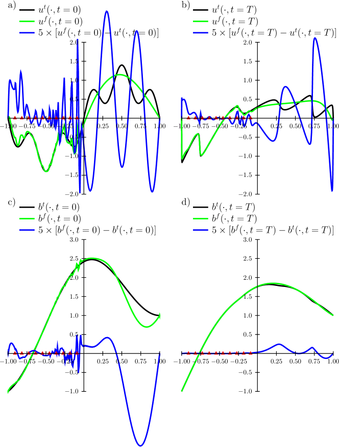
The lack of transmission of information from the left-hand side of the domain to its right-hand side is related to the short duration of model integration ( magnetic diffusion time, which corresponds to advective diffusion time with our choice of ). We shall comment further on the relevance of this remark for the assimilation of the historical geomagnetic secular variation in the discussion.
The lack of observational constraint on the right-hand side of the domain results sometimes in final errors larger than the initial ones (compare in particular Figs. 7a and 7b, with Figs. 4a and 4b).
We also note large error oscillations located at the interface between the left (sampled) and right (not sampled) regions, particularly at initial model time (Figs. 7a and 7c). The contrast in spatial coverage is likely to be the cause of these oscillations (for which we do not have a formal explanation); this type of behaviour should be kept in mind for future geomagnetic applications.
4.1.3 Irregular time sampling
We can also assume that the temporal sampling rate is not constant (keeping the spatial network of observatories homogeneous), restricting for instance drastically the epochs at which observations are made to the last % of model integration time, the sampling rate being ideal (that is performing observations at each model step). Not surprisingly, we are penalized by our total ignorance of the remaining per cent of the record. We illustrate the results obtained after assimilation with our now well-known array of stations by plotting the evolution of the errors in and (as defined above) versus time in Fig. 8.
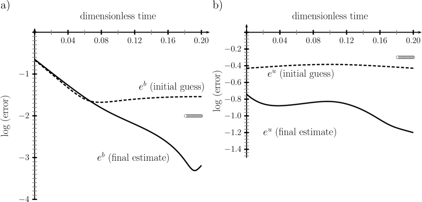
Although the same amount of information () has been collected to produce Figs. 5 and 8, the uneven temporal sampling of the latter has dramatic consequences on the improvement of the estimate of . In particular, the initial error remains large. The error decreases then linearly with time until the first measurement is made. We also observe that the minimum is obtained in the middle of the observation era. The poor quality of the temporal sampling, coupled with the not-sufficient spatial resolution obtained with these 20 stations, does not allow us to reach error levels as small as the ones obtained in Fig. 5, even at epochs during which observations are made. The velocity is sensitive to a lesser extent to this effect, with velocity errors being roughly times larger in Fig. 8 than in Fig. 5.
4.2 Imposing an a priori constraint on the state
As stated in Sect. 2, future applications of variational data assimilation to the geomagnetic secular variation might require to try and impose a priori constraints on the core state. In a kinematic framework, this is currently done in order to restrict the extent of the null space when trying to invert for the core flow responsible for the GSV (Backus, 1968; Le Mouël, 1984).
Assume for instance that we want to try and minimize the gradients of the velocity and magnetic fields, in a proportion given by the ratio of their diffusivities, that is the magnetic Prandtl number , at any model time. The associated cost function is written
| (50) |
in which is the derivative matrix introduced in §3.1.2. The total misfit reads, according to Eq. (5)
with as before, and , in which is the parameter that controls the constraint to observation weight ratio.
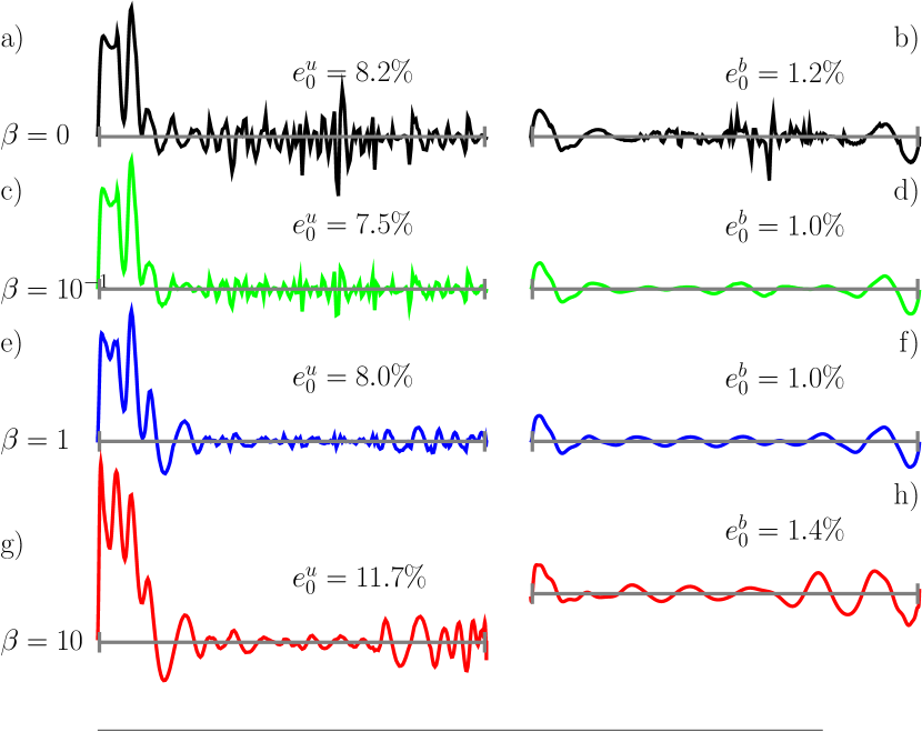
Response of the assimilated model to the imposed constraint is illustrated in Fig. 9, using the reference case of Fig. 4, for three increasing values of the parameter: and , and showing also for reference what happens when . We show the error fields (the scale is arbitrary, but the same for all curves) at the initial model time, for velocity (left panel) and magnetic field (right panel). The errors for each field at the end of assimilation indicate that this particular constraint can result in marginally better estimate of the initial state of the model, provided that the value of the parameter is kept small. For , the initial magnetic field is much smoother than the one obtained without the constraint and makes more physical sense (Fig. 9d). The associated velocity field remains spiky, with peak to peak error amplitudes strongly reduced in the heart of the computational domain (Fig. 9c). This results in smaller errors (reduction of about for and for ). Increasing further the value of leads to a magnetic field that is too smooth (and an error field even dominated by large-scale oscillations, see Fig. 9h), simply because too much weight has been put on the large-scale components of . The velocity error is now also smooth (Fig. 9g), at the expense of a velocity field being further away from the sought solution (%), especially in the left Hartmann boundary layer.
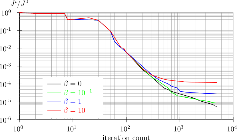
In the case of real data assimilation (as opposed to the synthetic case here, the true state of which we know, and departures from which we can easily quantify), we do not know the true state. To get a feeling for the response of the system to the imposition of an extra constraint, it is nevertheless possible to monitor for instance the convergence behaviour during the descent. On Fig. 10, the ratio of the misfit to its initial value is plotted versus the iteration number in the conjugate gradient algorithm (log-log plot). If is small, the misfit keeps on decreasing, even after 5,000 iterations (green curve). On the other hand, a too strong a constraint (blue and red curves in Fig. 10) is not well accommodated by the model and results in a rapid flattening of the convergence curve, showing that convergence behaviour can be used as a proxy to assess the efficacy of an a priori imposed constraint.
Again, we have used the constraint given by Eq. (50) for illustrative purposes, and do not claim that this specific low-pass filter is mandatory for the assimilation of GSV data. Similar types of constraints are used to solve the kinematic inverse problem of GSV (Bloxham and Jackson, 1991); see also Pais et al. (2004) and Amit and Olson (2004) for recent innovative studies on the subject. The example developed in this section aims at showing that a formal continuity exists between the kinematic and dynamical approaches to the GSV.
4.3 Convergence issues
In most of the cases presented above, the iteration counts had reached before the cost function had decreased by orders of magnitude. Even though the aim of this paper is not to address specifically the matter of convergence acceleration algorithms, a few comments are in order, since is too large a number when considering two- or three-dimensional applications.
-
•
In many cases, a reduction of the initial misfit by only orders of magnitude gives rise to decent solutions, obtained typically in a few hundreds of iterations. For example, in the case corresponding to Fig. 4, a decrease of the initial misfit by orders of magnitude is obtained after iterations. The resulting error levels are already acceptable : , , , and .
-
•
More importantly, in future applications, convergence will be sped up through the introduction of a background error covariance matrix , resulting in an extra term (Ide et al., 1997)
added to the cost function (Eq. (5)). Here, denotes the background state at model time , the definition of which depends on the problem of interest. In order to illustrate how this extra term can accelerate the inversion process, we have performed the following assimilation experiment: we take the network of virtual observatories of Fig. 4, and define the background state at model time to be zero for the velocity field (which is not directly measured), and the polynomial extrapolation of the magnetic observations made at the stations on the GLL grid points for the magnetic field (resorting to Lagrangian interpolants defined by the network of stations). The background error covariance matrix is chosen to be diagonal, without cross-covariance terms. This approach enables a misfit reduction by orders of magnitude in 238 iterations, with the following error levels : , , , and . This rather crude approach is beneficial for a) the computational cost and b) the estimate of the magnetic field. The recovery of the velocity is not as good as it should be, because we have made no assumption at all on the background velocity field. In future applications of VDA to the GSV, some a priori information on the background velocity field inside the core will have to be introduced in the assimilation process. The exact nature of this information is beyond the scope of this study.
5 Summary and conclusion
We have laid the theoretical and technical bases necessary to apply variational data assimilation to the geomagnetic secular variation, with the intent of improving the quality of the historical geomagnetic record. For the purpose of illustration, we have adapted these concepts (well established in the oceanographic and atmospheric communities) to a one-dimensional nonlinear MHD model. Leaving aside the technical details exposed in section 3, we can summarize our findings and ideas for future developments as follows:
-
•
Observations of the magnetic field always have a positive impact on the estimate of the invisible velocity field, even if these two fields live at different length scales (as could be expected from the small value of the magnetic Prandtl number).
-
•
With respect to a purely kinematic approach, having successive observations dynamically related by the model allows one to partially overcome errors due to a poor spatial sampling of the magnetic field. This is particularly encouraging in the prospect of assimilating main geomagnetic field data, the resolution of which is limited to spherical harmonic degree (say), because of (remanent or induced) crustal magnetization.
-
•
Over the model integration time ( % of an advection time), regions poorly covered exhibit poor recoveries of the true fields, since information does not have enough time to be transported there from well covered regions. In this respect, model dynamics clearly controls assimilation behaviour. Concerning the true GSV, the time window we referred to in the introduction has a width of roughly a quarter of an advective time scale. Again, this is rather short to circumvent the spatial limitations mentioned above, if advective transport controls the GSV catalog. This catalog, however, could contain the signature of global hydromagnetic oscillations (Hide, 1966; Finlay and Jackson, 2003), in which case our hope is that problems due to short duration and coarse spatial sampling should be alleviated. This issue is currently under investigation in our simplified framework, since the toy model presented here supports Alfvén waves.
-
•
A priori imposed constraints (such as the low-pass filter of Sect. 4.2) can improve assimilation results. They make variational data assimilation appear in the formal continuity of kinematic geomagnetic inverse problems as addressed by the geomagnetic community over the past years.
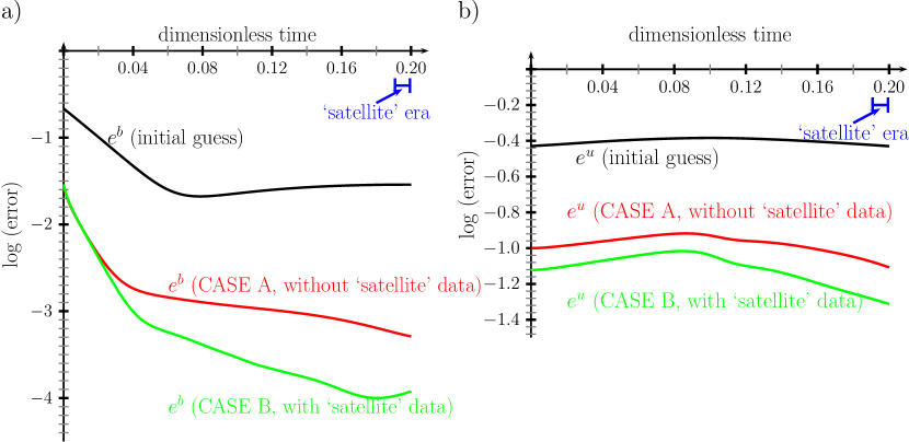
Finally, in order to illustrate the potential interest of applying VDA techniques to try and improve the recent GSV record, we show in Fig. 11 the results of two synthetic assimilation experiments. These are analogous to the ones described in great length in Sect. 4 (same physical and numerical parameters, constraint parameter ). In both cases, observations are made by a network of evenly distributed stations during the first half of model integration time (the logbooks era, say). The second half of the record is then produced by a network of stations for case A (the observatory era). For case B, this is also the case, save that the last % of the record are obtained via a high-resolution network of stations. The two records therefore only differ in the last % of model integration time. Case B is meant to estimate the potential impact of the recent satellite era on our description of the historical record.
The evolution of the magnetic error backwards in time (Fig. 11a) shows that the benefit due to the dense network is noticeable over three quarters of model integration time, with an error reduction of roughly a factor of . The velocity field is (as usual) less sensitive to the better quality of the record; still, it responds well to it, with an average decrease of on the order of %, evenly distributed over the time window.
Even if obtained with a simplified model (bearing in particular in mind that real geomagnetic observations are only available at the core surface), these results are promising and indicate that VDA should certainly be considered as the natural way of using high-quality satellite data to refine the historical geomagnetic record in order to ‘reassimilate’ (Talagrand, 1997) pre-satellite observations. To do so, a good initial guess is needed, which is already available (Jackson et al., 2000); also required is a forward model (and its adjoint) describing the high-frequency physics of the core. This model could either be a full three-dimensional model of the geodynamo, or a two-dimensional, specific model of short-period core dynamics, based on the assumption that this dynamics is quasi-geostrophic (Jault, 2006). The latter possibility is under investigation.
Acknowledgements
We thank Andrew Tangborn and an anonymous referee for their very useful comments, and Élisabeth Canet, Dominique Jault, Alexandra Pais, and Philippe Cardin for stimulating discussions. AF also thanks Éric Beucler for sharing his knowledge of inverse problem theory, and Élisabeth Canet for her very careful reading of the manuscript.
This work has been partially supported by a grant from the Agence Nationale de la Recherche (”white” research program VS-QG, grant reference BLAN06-2_155316).
All graphics were produced using the freely available pstricks and pstricks-add packages.
References
- Amit and Olson (2004) Amit, H. and Olson, P.: Helical core flow from geomagnetic secular variation, Phys. Earth Planet. Inter., 147, 1–25, doi:10.1016/j.pepi.2004.02.006, 2004.
- Anderson et al. (1999) Anderson, E., Bai, Z., Bischof, C., Blackford, S., Demmel, J., Dongarra, J., Du Croz, J., Greenbaum, A., Hammarling, S., McKenney, A., and Sorensen, D.: LAPACK Users’ Guide, Society for Industrial and Applied Mathematics, Philadelphia, PA, third edn., 1999.
- Backus (1968) Backus, G. E.: Kinematics of geomagnetic secular variation in a perfectly conducting core, Proc. Roy. Soc. London, A263, 239–266, 1968.
- Backus et al. (1996) Backus, G. E., Parker, R., and Constable, C.: An Introduction to Geomagnetism, Cambridge Univ. Press, 1996.
- Bennett (2002) Bennett, A. F.: Inverse Modeling of the Ocean and Atmosphere, Cambridge Univ. Press, Cambridge, 2002.
- Bloxham (1989) Bloxham, J.: Simple models of fluid flow at the core surface derived from field models, Geophys. J. Int., 99, 173–182, 1989.
- Bloxham (1998) Bloxham, J.: Dynamics of angular momentum of the Earth’s core, Annu. Rev. Earth Planet. Sci., 26, 501–517, 1998.
- Bloxham and Jackson (1991) Bloxham, J. and Jackson, A.: Fluid flow near the surface of Earth’s outer core, Rev. Geophys., 29, 97–120, 1991.
- Bloxham et al. (1989) Bloxham, J., Gubbins, D., and Jackson, A.: Geomagnetic Secular Variation, Philos. Trans. Roy. Soc. London, A329, 415–502, 1989.
- Brasseur (2006) Brasseur, P.: Ocean Data Assimilation using Sequential Methods based on the Kalman Filter, in: Ocean Weather Forecasting: An Integrated View of Oceanography, edited by Chassignet, E. and Verron, J., pp. 271–316, Springer–Verlag, 2006.
- Deville et al. (2002) Deville, M. O., Fischer, P. F., and Mund, E. H.: High-Order Methods for Incompressible Fluid Flow, vol. 9 of Cambridge monographs on applied and computational mathematics, Cambridge Univ. Press, Cambridge, 2002.
- Eymin and Hulot (2005) Eymin, C. and Hulot, G.: On core surface flows inferred from satellite magnetic data, Phys. Earth Planet. Inter., 152, 200–220, doi:10.1016/j.pepi.2005.06.009, 2005.
- Finlay and Jackson (2003) Finlay, C. C. and Jackson, A.: Equatorially dominated magnetic field change at the surface of earth’s core, Science, 300, 2084–2086, 2003.
- Greenspan (1990) Greenspan, H. P.: The Theory of Rotating Fluids, Breukelen Press, Brookline, MA, second edn., 1990.
- Hide (1966) Hide, R.: Free hydromagnetic oscillations of the Earth’s core and the theory of the geomagnetic secular variation, Philos. Trans. Roy. Soc. London, A259, 615–647, 1966.
- Ide et al. (1997) Ide, K., Courtier, P., Ghil, M., and Lorenc, A. C.: Unified Notation for Data Assimilation: Operational, Sequential and Variational, J. Meteorol. Soc. Japan, 75, 181–189, 1997.
- Jackson et al. (2000) Jackson, A., Jonkers, A., and Walker, M.: Four Centuries of Geomagnetic Secular Variation from Historical Records, Proc. Roy. Soc. London, A358, 957–990, 2000.
- Jault (2006) Jault, D.: On Dynamical Models of the secular variation of the earth’s magnetic field, in: Proceedings of the first Swarm International Science meeting, Nantes, 2006.
- Jault et al. (1988) Jault, D., Gire, C., and Le Mouël, J. L.: Westward drift, core motions and exchanges of angular momentum between core and mantle, Nature, 333, 353–356, doi:10.1038/333353a0, 1988.
- Le Mouël (1984) Le Mouël, J.-L.: Outer core geostrophic flow and secular variation of Earth’s magnetic field, Nature, 311, 734–735, 1984.
- Liu et al. (2007) Liu, D., Tangborn, A., and Kuang, W.: Observing System Simulation Experiments in Geomagnetic Data Assimilation, J. Geophys. Res., submitted, 2007.
- Maus et al. (2005) Maus, S., Lühr, H., Balasis, G., Rother, M., and Mandea, M.: Introducing POMME, the POstam Magnetic Model of the Earth, in: Earth observations with CHAMP, edited by Reigber, C., Lühr, H., Schwintzer, P., and Wickert, J., pp. 293–298, Springer, Berlin, 2005.
- Merrill et al. (1996) Merrill, R., McElhinny, M., and McFadden, P.: The magnetic field of the Earth, Academic Press, New York, 1996.
- Olsen et al. (2000) Olsen, N., Holme, R., Hulot, G., Sabaka, T., Neubert, T., Tøffner-Clausen, L., Primdahl, F., Jørgensen, J., Léger, J.-M., Barraclough, D., Bloxham, J., Cain, J., Constable, C., Golovkov, V., Jackson, A., Kotzé, P., Langlais, B., Macmillan, S., Mandea, M., Merayo, J., Newitt, L., Purucker, M., Risbo, T., Stampe, M., Thomson, A., and Voorhies, C.: Ørsted initial field model, Geophys. Res. Lett., 27, 3607–3610, doi:10.1029/2000GL011930, 2000.
- Olsen et al. (2006a) Olsen, N., Lühr, H., Sabaka, T. J., Mandea, M., Rother, M., Tøffner-Clausen, L., and Choi, S.: CHAOS-a model of the Earth’s magnetic field derived from CHAMP, Ørsted, and SAC-C magnetic satellite data, Geophys. J. Int., 166, 67–75, doi:10.1111/j.1365-246X.2006.02959.x, 2006a.
- Olsen et al. (2006b) Olsen, N., Haagmans, R., Sabaka, T., Kuvshinov, A., Maus, S., Purucker, M., Rother, M., Lesur, V., and Mandea, M.: The Swarm End-to-End mission simulator study: A demonstration of separating the various contributions to Earth’s magnetic field using synthetic data, Earth Planets Space, 58, 359–370, 2006b.
- Pais et al. (2004) Pais, M. A., Oliveira, O., and Nogueira, F.: Nonuniqueness of inverted core-mantle boundary flows and deviations from tangential geostrophy, J. Geophys. Res., 109, 8105–+, doi:10.1029/2004JB003012, 2004.
- Poirier (1988) Poirier, J.-P.: Transport properties of liquid metals and viscosity of the Earth’s core, Geophys. J. Roy. Astron. Soc., 92, 99–105, 1988.
- Roberts and Scott (1965) Roberts, P. H. and Scott, S.: On analysis of the secular variation, Journal of geomagnetism and geoelectricity, 17, 137–151, 1965.
- Shewchuk (1994) Shewchuk, J. R.: An Introduction to the Conjugate Gradient Method Without the Agonizing Pain, Tech. rep., Carnegie Mellon University, Pittsburgh, PA, USA, 1994.
- Sun et al. (2007) Sun, Z., Tangborn, A., and Kuang, W.: Data assimilation in a sparsely observed one-dimensional modeled MHD system, Nonlin. Processes Geophy., submitted, 2007.
- Talagrand (1997) Talagrand, O.: Assimilation of observations, an introduction, J. Meteorol. Soc. Japan, 75, 191–209, 1997.
- Talagrand and Courtier (1987) Talagrand, O. and Courtier, P.: Variational assimilation of meteorological observations with the adjoint vorticity equation. I: Theory, Quart. J. Roy. Meteorol. Soc., 113, 1311–1328, 1987.