SLE in the three-state Potts model - a numerical study

Abstract

The scaling limit of the spin cluster boundaries of the Ising model with domain wall boundary conditions is SLE with $\kappa=3$. We hypothesise that the three-state Potts model with appropriate boundary conditions has spin cluster boundaries which are also SLE in the scaling limit, but with $\kappa=10/3$. To test this, we generate samples using the Wolff algorithm and test them against predictions of SLE: we examine the statistics of the Loewner driving function, estimate the fractal dimension and test against Schramm’s formula. The results are in support of our hypothesis.

1 Introduction

Much of the recent interest in Schramm Loewner evolution (SLE) stems from the description it offers of cluster boundaries in critical statistical mechanics models. These models are conjecturally described by conformal field theories, which determines expectation values of products of local operators. However, non-local objects such as cluster boundaries do not have a natural expression in the field theory language. These curves are of great interest as, for example, they describe percolation cluster boundaries, level lines of height models and spin cluster boundaries. Recently, the scaling limit of the spin cluster boundary in the Ising model with appropriate boundary conditions has been proven to be SLE with $\kappa=3$ [8].

The Ising model corresponds to the $q$-state Potts model with $q=2$. We may ask, therefore, whether spin boundaries in the critical Potts model with other values of $q$ have SLE as their scaling limit. The Fortuin-Kastelyn (FK) cluster representation [4] of the Potts model contains closed loops which may be taken to be the contours of a suitably defined height model. The scaling limit of this model is supposed to be a field theory (CFT) called the Coulomb gas which possesses a single parameter $g$, where $\sqrt{q}=-2\cos(\pi g)$. The connection with SLE is that the winding angle of these loops in the Coulomb gas are equivalent to that seen in radial SLE for $\kappa=4/g$. Therefore, we have reason to believe that the FK cluster boundaries should correspond to SLE in the scaling limit, with

$$\kappa=\frac{4}{1-\arccos(\sqrt{q}/2)/\pi}\,.$$ (1)

The spin cluster boundaries are related to these FK cluster boundaries in a non-trivial way, however, and it is therefore interesting to investigate the properties of these spin boundaries in the scaling limit. For the Ising model, these spin cluster boundaries are also described by SLE at the dual value $\kappa^{\prime}=16/\kappa$ [8].

Besides $q=1$ (corresponding to percolation), there are two other integer values of $q$ for which the Potts model displays a continuous phase transition: $q=3$ and $q=4$ (for $q>4$ the transition is first order). In this paper, we investigate the case $q=3$ and test for agreement of numerically simulated lattice spin cluster boundaries with known predictions of SLE. The dual value of $\kappa$ for $q=3$ is, from equation 1 above, $\kappa^{\prime}=16/\kappa=10/3$. We may hypothesise, therefore, that the spin cluster boundaries, properly defined, of the $q=3$ Potts model are SLE with $\kappa=10/3$. This paper is a numerical investigation of that prediction.

The set-up of chordal SLE requires that the curves connect fixed points on the boundary of a simply connected domain. This is ensured by careful choice of the boundary conditions. For example, consider the following boundary conditions for the Ising model: divide the boundary into two connected subsets (‘left’ and ‘right’). Let the left boundary spins be spin up and the right boundary spins be spin down. This ensures that a spin cluster boundary runs from one fixed point on the boundary to another, for every configuration of the bulk spins. The Gibbs distribution induces a measure on these curves. The case of the $q=3$ Potts model is similar, although there are now two types of interesting boundary conditions. If the boundary conditions are chosen as for the Ising model, with those on the left part being of spin type $1$ (say) and those on the right of spin type $2$, the right boundary curve of the cluster connected to the boundary spins of type $1$ does not everywhere coincide with the right boundary curve of those of type $2$. In other words, the spin cluster boundary may split around regions of spin type $3$, which themselves may contain islands of the other spin types, ad infinitum. One possibility for the scaling limit is that the two cluster boundaries are distinct, with probability one. This might then be expected to correspond to two-curve SLE. We therefore simulate numerically a set of samples with these boundary conditions and compare to predictions from two-curve SLE: the fractal dimensions and the formulae describing the expected spatial distribution of the curves in the bulk [5]. The other choice for boundary conditions is to fix the left set of the boundary spins to be of type $1$ and to allow those on the right to fluctuate between the other two spin types. In this case, we may consider the right boundary of the cluster connected to the boundary spins of type $1$, which forms a curve connecting the two fixed points on the boundary. The measure on this set of curves is, as before, induced by the Gibbs distribution. We also simulate Potts models with these boundary conditions to test against two predictions of single-curve SLE: the fractal dimension and Schramm’s formula. For the single curve case, we also examine the statistics of the driving function by undoing the sequence of conformal transformations which uniquely determine the form of the curve through the Loewner equation. This driving function should be Brownian motion with diffusivity $\kappa$ if the curves correspond to SLE.

The layout of the paper is as follows: In section 2, we summarise the definition and important features of the Potts model, explaining in detail the boundary conditions required to generate cluster boundaries. In section 3, we recall the definition of SLE and describe the predictions of SLE which we will test our samples against. In section 4 we describe the details of the numerical simulations we performed, explaining how the fractal dimension and other data are extracted from the generated samples. In section 5, we present the results of our numerical simulations and conclude in section 6. The appendix contains details of the Wolff algorithm used for all simulations.

2 The Potts model

The $q$-state Potts model is a lattice spin model. The spins may take values from the set $\{1,2...,q\}$ and have nearest neighbour interactions, such that the partition function takes the form

$$Z=\textrm{Tr}\,e^{J\,\sum_{r,r^{\prime}}{\delta_{s(r),s(r^{\prime})}}}\,.$$ (2)

$J$ is the reduced coupling constant and $\delta_{i,j}$ is the Kronecker delta. The case $q=2$ is equivalent to the Ising model, up to a constant. For $q>2$, therefore, the Potts model describes a generalisation of the Ising model to systems with more than two spin types. For a given $q\leq 4$ and choice of lattice, there exists a value of the coupling constant, $J_{c}$, at which the model has a continuous transition; the two point correlation function of the spins decays as a power law and the scaling limit of the model is supposed to be described by a conformal field theory. For later reference, these values for the two lattice types considered in this work are [11]

• Square lattice $e^{J_{c}}=\sqrt{q}+1$.

• Triangular lattice $e^{J_{c}}=2\cos(\frac{2}{3}\cos^{-1}(\sqrt{q}/2))$.

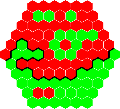
Let us consider spin cluster boundaries in the Ising model arising from a specific choice of boundary conditions. Namely, let those spins on a connected piece of the boundary be of spin type $1$ and elsewhere on the boundary, the spins be of type $2$. This is demonstrated in figure 1, where spin type $1$ is represented by the colour red and type $2$ spins are coloured green. Then, for every configuration of the spins in the bulk, there exists a unique curve starting and ending at two fixed points on the boundary. Immediately to one side of the curve, all the spins are green. To the other side, the spins are red. The measure on these curves is derived from the Gibbs distribution.

Figure 1: The Ising model with boundary conditions as in the text. The spins are represented by hexagons, so that there are six nearest neighbours for each spin in the bulk. Half of the boundary spins are of type $1$ (coloured red, or dark grey on black and white printouts) and the others of type $2$ (green or light grey). There exists a boundary of the cluster connected to the bottom edge (the thick black line) which coincides with the boundary of the cluster connected to the top edge. This curve connects the same two points on the boundary for every configuration of the bulk spins.

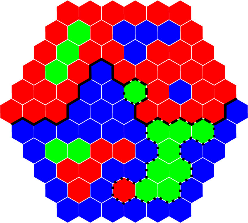
Let us consider how to define the boundary conditions for the $q=3$ Potts model in such a way as to guarantee the existence of cluster boundary curves propagating through the sample. The natural extension of the boundary conditions for the Ising model is to fix a connected set of the boundary spins to be of (say) spin type $1$ (red or dark grey on black and white printouts), with the remaining spins of type $3$ (blue or black), as in figure 2. The particular choice of spins is, of course, arbitrary due to the $S_{3}$ symmetry of the model. We shall refer to these boundary conditions as ‘fixed’ boundary conditions. However, the situation is different from the Ising model, since in this case the boundary curve of the cluster containing the red boundary spins does not always coincide with the boundary of the cluster containing the blue boundary spins. In the figure, the dotted line is the boundary of the cluster containing the blue boundary spins, the dashed line is the boundary of the cluster containing the red boundary spins and where the two curves are both present along an edge, a thick black line has been drawn. This black line is reminiscent of the single cluster boundary in the Ising model, with spins immediately to one side of it red and those on the other side being blue, but the dotted and dashed lines are of a new type. The dotted line has blue spins to one side and either green (light grey on black and white printouts) or red to the other. The dashed line has red spins to one side and either green or blue to the other side. In this paper, we shall refer to the thick black lines as the ‘composite’ cluster boundaries and the dashed and dotted lines as the ‘split’ cluster boundaries. Note that the ‘composite’ cluster boundary splits into two ‘split’ cluster boundaries whenever it encounters a vertex with all three spin types, and that a pair of ‘split’ cluster boundaries recombine only at such three spin vertices.

Figure 2: The $q=3$ Potts model with ‘fixed’ boundary conditions. The clusters connected to the bottom and top edges are no longer everywhere overlapping. The dashed and dotted lines are ‘split’ cluster boundaries. The thick black line is the ‘composite’ cluster boundary.

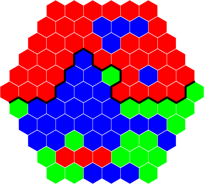
There exists another choice of boundary conditions for the $q=3$ Potts model which we will refer to as ‘fluctuating’ boundary conditions. A connected set of the boundary spins are set to be of spin type $1$ (red). The remaining boundary spins are allowed to fluctuate with the spins in the bulk, but are not permitted to be of type $1$. They are therefore of type $2$ (green) or $3$ (blue), see figure 3. The cluster boundary of the red spin cluster connected to the top edge now coincides with the boundary of a cluster comprised of green and blue spins connected to the bottom edge, which is defined as follows: replace all green and blue spins with a new spin type $x$ and consider the boundary of the cluster of $x$ spins connected to the bottom edge. That these two cluster boundaries always coincide may be readily seen by analogy with configurations of the Ising model with spin types red and $x$. The reader will note the lack of reflection symmetry in the boundary conditions. This may be expected to lead to non-reflection symmetric spin cluster boundary curves. However, we shall present evidence that these curves are actually reflection symmetric in the scaling limit.

Figure 3: The $q=3$ Potts model with ‘fluctuating’ boundary conditions. There exists a single uniquely defined boundary curve between the red (dark grey) cluster and the green (light grey) and blue (black) cluster, as defined in the text.

3 Schramm Loewner evolution

We expect the cluster boundary curves of critical statistical models to be described by measures which are invariant under conformal transformations, due to the conformal invariance of the action associated to these models. This argument can be made more precise; the changes in boundary conditions described in the previous section have been shown [2, 6] to be produced by the insertion of boundary $\phi_{1,2}$ operators in the appropriate conformal field theory. Expectation values of observables therefore correspond to correlation functions with a pair of these boundary condition changing operators inserted. It may be shown, for a specific choice of observables, that the partial differential equations for these correlation functions arising from the null state associated with the $\phi_{1,2}$ operators are the same as those coming from the mathematical theory of random curves with conformally invariant measure, known as Schramm Loewner evolution (SLE).

Let us summarise the main features of the theoretical physicist’s version[3, 1] of SLE. A curve in the upper half plane from the origin to infinity is considered as being grown dynamically as a function of time $t$, which therefore parameterizes distance along the curve. Let $K_{t}$ be the set consisting of the curve as grown up to time $t$ (as well as all points enclosed by the curve and between the curve and the real axis) so that the complement of this set in the upper half plane is simply connected. Let $g_{t}(z)$ be the (unique) conformal mapping of this complement to the whole upper half plane, normalised such that $g_{t}(z)=z+O(1/z)$ as $z\to\infty$. The coefficient of the $O(1/z)$ term is increasing with $t$, so ‘time’ can be reparametrised such that this coefficient is exactly $2t$. Then, $t$ is known as the capacity. The image of the growing tip of the curve under $g_{t}$ is a point $a_{t}$ on the real axis. Loewner showed that the time-evolution of $g_{t}$ satisfies a differential equation, which is named after him:

$$\frac{dg_{t}(z)}{dt}=\frac{2}{g_{t}(z)-a_{t}}\,.$$ (3)

Any suitably continuous function $a_{t}$ generates a curve. Schramm[7] showed that for this process to generate a conformally invariant measure on curves, the driving function must be $a_{t}=\sqrt{\kappa}B_{t}+a_{0}$, with $B_{t}$ being a standard Brownian motion.

There remains a single parameter in the theory, $\kappa$, which is the diffusivity of the Brownian motion. A small value of $\kappa$ results in a measure which favours curves with few turns, whereas a large value of $\kappa$ leads to a measure favouring curves which wind more frequently, touching themselves and the real axis. The value of $\kappa$ is conjecturally related to the central charge of the conformal field theory it describes via the formula:

$$c=\frac{(3\kappa-8)(6-\kappa)}{2\kappa}\,.$$ (4)

From this formula, it is clear that the central charge associated to an SLE with diffusivity $\kappa$ is equal to that of the dual SLE with $\kappa^{\prime}=16/\kappa$.

We will now describe some properties of SLE curves.

3.1 The fractal dimension

If $N(r)$ is the number of discs of radius $r$ required to cover an object, this number scales as $N(r)\sim r^{-d_{f}}$ for small $r$, where the exponent $d_{f}$ is known as the fractal dimension. SLE curves are fractal objects, with

$$d_{f}=1+\frac{\kappa}{8}\,,\quad\textrm{for}\,\kappa\leq 8\,.$$ (5)

The total length of the curve, $S$, measured in units of the lattice spacing, $a$, obeys a scaling relation as a function of system size, $L$, as $L/a\rightarrow\infty$

$$S\sim a\left(\frac{L}{a}\right)^{d_{f}}\,.$$ (6)

3.2 Schramm’s formula

Schramm’s formula relates to the following question: given an SLE connecting two boundary points, what is the probability that the curve passes to one side of a point, $\xi(z)$, in the interior? If the domain is mapped to the upper half plane such that the SLE connects $0$ to $\infty$, this probability may be expressed as the solution to a second order partial differential equation. Let us consider the probability that the curve passes to the left of a point, $P_{\rm left}$. By this we mean that there is a continuous path from the point to the positive real axis which does not intersect the SLE curve. The solution is found by applying appropriate boundary conditions to the solution to the differential equation, which is a function only of $t\equiv{\textrm{R}e}(\xi)/{\textrm{I}m}(\xi)$ due to the conformal invariance of the measure:

$$P_{\rm left}(t)=\frac{1}{2}-\frac{\Gamma(\frac{4}{\kappa})}{\sqrt{\pi}\Gamma(\frac{8-\kappa}{2\kappa})}t\,_{2}F_{1}(\frac{1}{2},\frac{4}{\kappa};\frac{3}{2};-t^{2})\,.$$ (7)

The two domains considered in this work are related to the upper half plane by simple transformations, hence this result may be re-expressed easily in terms of the conventional coordinates in these domains.

The generalisation of this result to the two-SLE case, was the subject of a recent paper[5]. Given a pair of SLEs both connecting $0$ to $\infty$ in the upper half plane, there are three possibilities: an interior point, $\xi(z)$, may be to the left of both curves, between them or to the right hand side of both. There is a probability for the curve to belong to each class, which is a function only of $t\equiv Re(\xi)/Im(\xi)$, just as for the single curve case. The probability of each class obeys a third order linear partial differential equation, with solutions which are integrals of hypergeometric functions. The particular solution of interest is found by imposing a natural set of boundary conditions, namely the asymptotic behaviour as the point approaches the positive and negative real axis. The solutions are

$$P_{\textrm{left}}(t)=\frac{\Gamma(\frac{4}{\kappa})\Gamma(\frac{8}{\kappa})}{2^{2-8/\kappa}\pi\Gamma(\frac{12}{\kappa}-1)}\int_{t}^{\infty}S(t^{\prime})\textrm{d}t^{\prime}\,,$$ (8)

where

$$S(t)=\frac{\,{}_{2}F_{1}(\frac{1}{2}+\frac{4}{\kappa},1-\frac{4}{\kappa};\frac{1}{2};-t^{2})-\frac{2\Gamma(1+\frac{4}{\kappa})\Gamma(\frac{4}{\kappa})}{\Gamma(\frac{1}{2}+\frac{4}{\kappa})\Gamma(-\frac{1}{2}+\frac{4}{\kappa})}\,t\,_{2}F_{1}(1+\frac{4}{\kappa},\frac{3}{2}-\frac{4}{\kappa};\frac{3}{2};-t^{2})}{(1+t^{2})^{\frac{8}{\kappa}-1}}\,,$$

and

$$P_{\textrm{middle}}(t)=1-\frac{\Gamma(\frac{4}{\kappa})\Gamma(\frac{8}{\kappa})}{2^{2-8/\kappa}\pi\Gamma(\frac{12}{\kappa}-1)}\Big{[}\int_{t}^{\infty}S(t^{\prime})dt^{\prime}+\int_{-t}^{\infty}S(t^{\prime})dt^{\prime}\Big{]}\,.$$ (9)

The probability that the curves are both to the right of a point may be deduced from the other two cases. Throughout this paper, we shall refer to these equations as the two-curve formulae. As for the single curve formula, the results may be transferred to the domains of interest via a conformal transformation.

3.3 4-leg operators

Consider the $q=3$ Potts model with ‘fixed’ boundary conditions. There are a pair of cluster boundary curves in this case, which initially overlap, taking the form of a ‘composite’ cluster boundary. This may be expected to split around a cluster of spins which is not connected to the boundary. We may ask about the relevance, in a renormalization group sense, of the operator responsible for the recombination of these ‘split’ curves. This operator is familiar from the height representation of the $O(n)$ model, where it is known as the 4-leg operator. The scaling dimension of this 4-leg operator is

$$x_{4}=2g-\frac{(g-1)^{2}}{2g}\,$$ (10)

where $g=1-\arccos{(\sqrt{q}/2)}/\pi$. For $q=4$, which we do not consider in this paper, the 4-leg operator is therefore marginal with $x_{4}=2$, since $g=1$ in this case. For $q=3$, the scaling dimension is $x_{4}=99/60$, which means it is irrelevant. As the system size increases, the ‘split’ boundary curves are therefore expected to collide less frequently. We may expect the scaling limit in this case to correspond to a pair of non-intersecting SLE curves. Note that the joining of two ‘split’ curves and a ‘composite’ curve at a point does not correspond to the insertion of a 3-leg operator, since the two types of curves are inequivalent. Indeed, we shall see that the ‘composite’ curve has a different fractal dimension.

4 Numerical simulations

We use the algorithm described in appendix B to generate a representative set of spin configurations at the critical point of the $q$-state Potts model for both $q=2$ and $q=3$ in two domains. The first is the square lattice on the rectangle with aspect ratio $3:1$, the second is the triangular lattice on the disc.

As explained in section 2, if the boundary conditions for $q=2$ (the Ising model) are chosen appropriately, a continuous boundary curve separating the two spin clusters runs between two points on the boundary. This ensemble of curves has recently been proven to converge to SLE₃ [8]. It is therefore a useful check to show that the set of boundary curves obtained from our algorithm for $q=2$ satisfy the expected properties of SLE, as outlined in section 3.

The main aim of this paper is to gather numerical support for the spin boundaries of the 3-state Potts model with appropriate boundary conditions becoming SLE in the scaling limit. There are two types of boundary conditions: ‘fluctuating’ boundary conditions (see section 2) lead to a single curve running between two boundary points. ‘Fixed’ boundary conditions lead to a pair of ‘split’ curves running between two fixed points on the boundary, which may overlap to form a ‘composite’ curve. In section 3.3 we presented an argument for only the ‘split’ curves being present in the scaling limit. We test the validity of this argument by comparing the fractal dimensions of the two types of curves.

The geometries chosen for the simulations are the square lattice on a narrow rectangular sample, and the triangular lattice on a disc. The first is chosen so that Schramm’s formula (see section 3.2) may be compared with that on an infinite strip. The second geometry is chosen for the ease of obtaining the driving function of single curves (see section 4.4). The two are complimentary in the sense that the measure on curves in the two domains should be related by the conformal transformation between them. That critical statistical models are conformally invariant is an accepted conjecture, but this does provide another useful check of the robustness of the algorithm, as well as a further demonstration that properties of the scaling limit of the curves are consistent with those of SLE.

The remainder of this section is dedicated to a technical discussion of the methods of obtaining data from the samples.

4.1 Identifying the cluster boundaries

Given a configuration of spins, the first step to identifying the boundary curves is to identify the extent of the cluster containing a given boundary spin. This is done using the following algorithm:

1. Start at the boundary spin of interest, marking it as belonging to the cluster

2. Mark all neighbours if they are of the same spin type

3. Repeat step 2 for all neighbours of marked spins

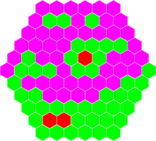
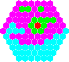
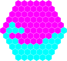
4. Identify all connected sets of unmarked spins which are surrounded by a closed path of marked spins. Mark all such sets of spins.

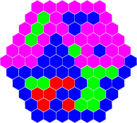
This process is demonstrated in figure 4 for an Ising sample.

      

                              (a)                                       (b)

      

                              (c)                                       (d)

Figure 4: (a) shows a spin configuration in the Ising model. To obtain (b), recolour a red boundary spin at the top of the sample purple. Recolour all its red neighbours purple and repeat for all their neighbours et cetera. To obtain (c), recolour a green spin on the bottom edge cyan. Recolour all its non-purple neighbours cyan and repeat for all their neighbours et cetera. Finally, to obtain (d), recolour all remaining green and red spins purple.

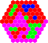
It is sufficient to identify a single cluster boundary for the Ising model and $q=3$ model with ‘fluctuating’ boundary conditions, since the cluster boundaries of the top and bottom clusters overlap everywhere in these cases (see section 2). For the case $q=3$ with ‘fluctuating’ boundary conditions, as in figure 3 for example, the first step to identifying the mixed spin cluster boundary is to replace all blue spins throughout the sample with green spins. Then, the algorithm is the same as that for the Ising model.

       

                 (a)                               (b)                               (c)

       

                 (d)                               (e)                               (f)

Figure 5: Figure (a) shows a $q=3$ Potts model spin configuration with ‘fixed’ boundary conditions. To obtain (b), recolour a red boundary spin at the top of the sample purple. Recolour all its red neighbours purple and their red neighbours purple et cetera. To obtain (c), recolour a blue spin on the bottom edge cyan and all its non-purple neighbours also. Repeat for all their non-purple neighbours et cetera. Recolour purple all the remaining red, blue and green spins. To identify the cluster containing the blue boundary spins, start again from figure (a). Fig (d) shows the result of starting with a blue spin on the bottom edge and recolouring all its blue neighbours purple, et cetera. Fig (e) is obtained after recolouring cyan all non-purple neighbours starting from a red spin at the top edge. Lastly, recolour all remaining red, blue and green spins purple. The two clusters connected to the boundary are coloured differently in figures (c) and (e). But some spins are cyan in both (c) and (e). These are yellow in figure (f). The top cluster is pink and the bottom cluster is grey.

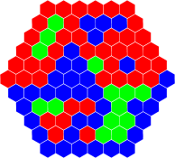
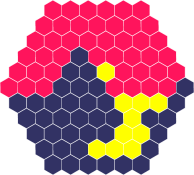
For the $q=3$ model with ‘fixed’ boundary conditions, however, this process must be run twice to identify both the cluster connected to the bottom edge of the sample and that connected to the top edge, see figure 5. The result is figure 5(f), which shows all three types of clusters present. Note that the example figures are for the triangular lattice case. The same algorithms to determine the cluster boundaries are employed for samples generated on the square lattice.

4.2 Estimating the fractal dimension

For the Ising model and the $q=3$ Potts model with ‘fluctuating’ boundary conditions, there is a single curve running between two fixed points on the boundary. First, identify the cluster containing one set of boundary spins, as outlined in section 4.1. This results in a configuration of the type shown in figure 4(d). Then, the length of the cluster boundary curve is deduced as follows. For each site on the sample, compare the colour at that site to each of its nearest neighbours. If the nearest neighbour is of the same colour (and therefore connected to the same cluster) there is not a cluster boundary separating the two spins. Otherwise, if it is of the other colour, add one half to the total length of the cluster boundary curve (since each link will be counted twice by this algorithm).

The situation for $q=3$ with ‘fixed’ boundary conditions involves the fractal dimension of two types of cluster boundaries: the ‘composite’ cluster boundaries and the ‘split’ cluster boundaries, see section 2. Identify the clusters containing the two types of boundary spin and also the clusters which do not contain a boundary spin. This leads to a cluster configuration similar to that shown in figure 5(f). The total length of ‘composite’ boundaries is found by summing over all sites, adding one half to a running total wherever a pink site is adjacent to a grey site. The total length of ‘split’ cluster boundaries is found by identifying all sites where a grey site is adjacent to a yellow site or a pink site is adjacent to a yellow site, adding one half to a different running total for each such occurence.

In this way, we may deduce the expected length of curves as a function of system size. Comparison to equation 6 allows an estimation of the fractal dimension of the curves.

4.3 Comparison to Schramm’s formula and its generalisation to two curves

Firstly, for the Ising model and $q=3$ Potts model with ‘fluctuating’ boundary conditions, the starting point is the cluster configuration picture, as in figure 4(d). Recall that the boundary conditions are chosen such that the curve starts and ends at opposite points on the boundary. There is a path which is equidistant from these two points, which is shown in figure 6 for the rectangle. For each site along this path, calculate the percentage of the samples for which the site is coloured cyan. This yields the fraction of samples for which this point is connected to the bottom cluster. This may be compared to the predictions of Schramm’s formula.

For the $q=3$ Potts model with ‘fixed’ boundary conditions, the procedure is to deduce the cluster picture, as in figure 5(f). Two separate quantities may be measured, the percentage of the samples for which each point along the path is connected to the bottom cluster (coloured grey) and the percentage which are in the central, yellow cluster. In the former case, the point is to one side of both curves (the left hand side say), whereas in the latter example, the points are between the two curves. These results are to be compared to the generalisation of Schramm’s formula to two curves, the two-curve formulae (see section 3.2).

4.4 The driving function

The third test is to analyse the driving function of the curves for the Ising model and $q=3$ Potts model samples with ‘fluctuating’ boundary conditions. The spin boundary curves have a natural discretisation provided by the lattice itself, so a curve may be approximated by the set of ordered lattice points which it passes through. It is easiest to consider the set of conformal mappings of the curve back to the boundary in the upper half plane, so the first step is to transform domains using a conformal transformation. For the disc, for example, this is the following Mobius transformation:

$$h(z)=\frac{z-1}{i(z+1)}\,.$$ (11)

For the rectangle, the transformation to the upper half plane is not so convenient; the derivative of the conformal map at the corners is large. The effect of this cannot be simply and systematically removed.

The curve grown up to a point $\gamma$ may be mapped back to the real axis by a series of vertical slit maps for each successive discretized point, $\chi_{i}$, along the curve

$$g_{i,t}(z)=\textrm{Re}(\chi_{i})+\sqrt{((z-\textrm{Re}(\chi_{i}))^{2}+\textrm{Im}(\chi_{i})^{2})}\,.$$ (12)

This maps the point $\chi_{i}$ to $\textrm{Re}(\chi_{i})$ on the real axis, which is therefore the value of the driving function, $a_{t}$, at the time when this point is the tip of the growing curve. The change in $t$ associated with this piece of curve is found from the expansion of the map as $z\rightarrow\infty$:

$$g_{t}(z\rightarrow\infty)=z+\frac{\textrm{Im}(\chi)^{2}/2}{z}+\ldots$$

The change in $t$ is therefore $\delta t=\textrm{Im}(\chi_{i})^{2}/4$. For SLE, the driving function should be a multiple of Brownian motion. In particular, the expectation value of $a_{t}$ should vanish and the variance should be $\kappa$. On a plot of frequency of step lengths (normalised by $\sqrt{\delta t}$) the distribution should be Gaussian with variance $\kappa t$. Our lattice curves are only supposed to approximate SLE at scales much larger than the lattice spacing. Therefore, effective steps equivalent to $10$ lattice steps are considered. $\delta B$ is then the change in the driving function as a result of an effective step, and $\delta t$ is the capacity change, totalled over the $10$ component steps. We also plot $\langle a_{t}^{2}\rangle$ as a function of $t$, with a view to equating the gradient to $\kappa$.

5 Results

In this section, we present a comparison between the results from the numerical simulations and predictions from SLE. The algorithm used to generate samples is described in appendix B.

5.1 Ising model on the rectangle

This section describes the results from the Ising model on the rectangle on a square lattice of aspect ratio $1:3$. Four system sizes are used: $40\times 120$, $60\times 180$, $80\times 240$ and $100\times 300$, where the lengths are in multiples of the lattice spacing. These will be referred to by their smaller dimension. The boundary conditions are as described in section 2, with one spin type fixed along a long edge and half each of the shorter sides, and the other spin type elsewhere. The geometry is therefore as shown in figure 6.

Figure 6: The geometry used for the Ising model on the rectangle of aspect ratio $1:3$ with a square lattice. The boundary conditions are shown, but the bulk spins left grey. The path used to test against Schramm’s formula is shown as the blue dashed line.

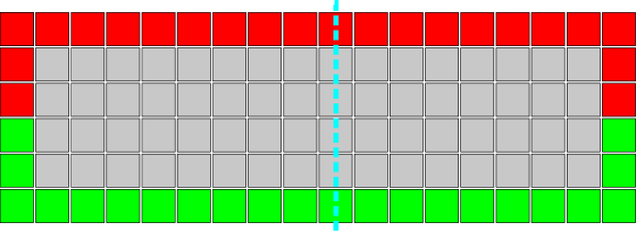
A cluster boundary curve runs from the centre of one short edge of the rectangle to the centre of the other short edge. $50,000$ independent samples of each system size are used to estimate the fractal dimension of the curves, by determining the average length as a function of system size. This process is explained in section 4.2. The results are plotted in figure 7. The error bars are shown, but are only just discernible at this magnification.

Figure 7: The fractal dimension of the Ising model on the rectangle. The system size is defined as the number of lattice spacings across the smaller side of the rectangle. The curve length is measured in multiples of lattice spacings.

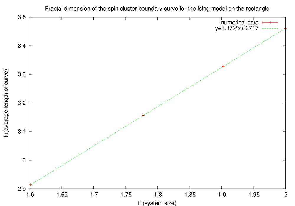
The linear fit is in good agreement with the data, with reduced $\chi^{2}$ equal to $0.7$. It shows a fractal dimension of $d_{f}=1.372\pm 0.002$. Using formula 5, this would correspond to SLE with $\kappa=2.976\pm 0.02$. The known value of $\kappa=3$ for the Ising model lies just outside these error bars.

The fit to Schramm’s formula is via the logarithmic map from the upper half plane to the infinite strip:

$$w(z)=\frac{\ln{z}}{\pi}\,.$$ (13)

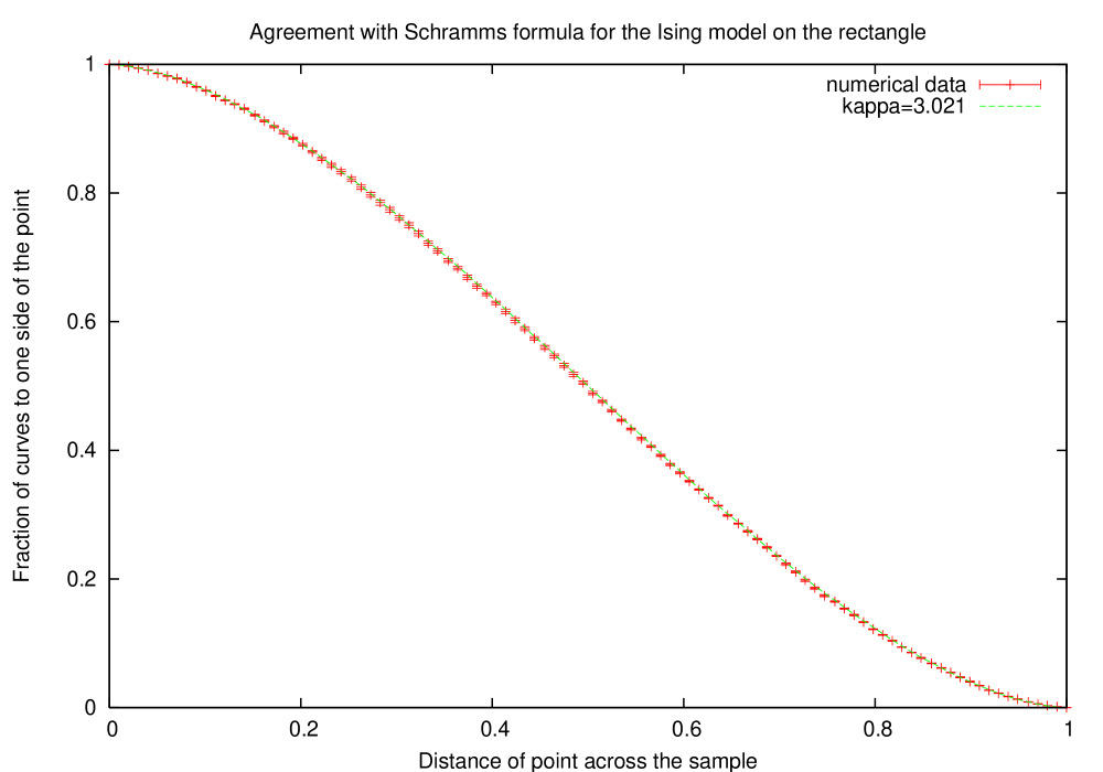
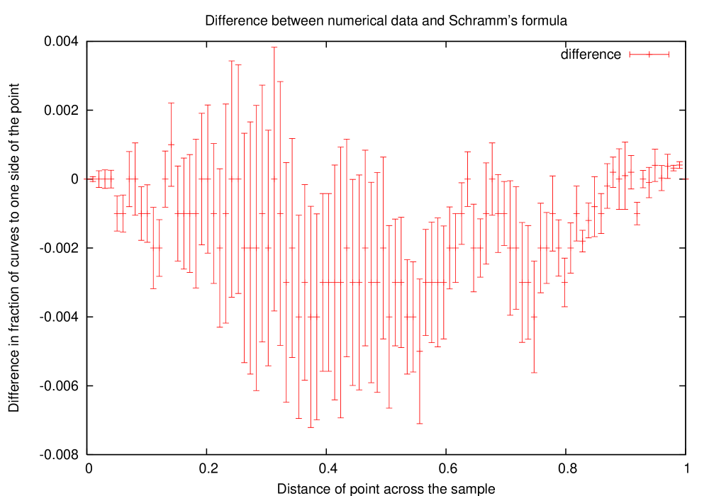
The assumption that the strip is effectively infinitely long is valid only if the boundary curve at the centre of the sample is independent of the boundary conditions at the ends of the rectangle. We tested this by generating system sizes of aspect ratios $1:5$ and $1:6$. The differences in the data are smaller than the error in the measurements. In terms of a coordinate, $s$, which describes the fractional distance across the strip, $t$ is given by $t=\cot(\pi s)$ in equation 7. This follows from equation 13. The results from the numerical data are the expectation value for the point at a fractional distance $s$ across the strip being connected to the bottom spin cluster. Figure 8 shows the comparison to the best fit value of $\kappa=3.021\pm 0.015$. Once more, the known value lies just outside this range. We should not be surprised, therefore, it the predicted value of $10/3$ for $q=3$ Potts model also lies just outside the range obtained from the numerics. The average is again over $50,000$ independent samples.

Figure 8: Fit to Schramm’s formula on the strip for the Ising model, system size $100\times 300$. The smaller system sizes also show good agreement with Schramm’s formula with $\kappa\approx 3.0$. The agreement is to approximately 1%, as shown in the lower figure.

5.2 $q=3$ on the rectangle

The geometry is the same as for the Ising model above, with sample sizes $40\times 120$, $60\times 180$, $80\times 240$ and $100\times 300$. First, let us examine the case of ‘fluctuating’ boundary conditions, when there is a single curve connecting two boundary points at the centre of each short end of the rectangle. The boundary conditions are like those in figure 6 except that the boundary spins on the bottom half are permitted to be either blue or green and to fluctuate with the spins in the bulk. The fractal dimension comes from the average length of the curves as a function of system size, where $50,000$ independent samples have been generated for each sample size. The results are shown in figure 9.

Figure 9: The fractal dimension of the $q=3$ Potts model on the rectangle with fluctuating boundary conditions. System size is the shorter side of the rectangle in units of lattice spacing. The curve length is in units of lattice spacings.

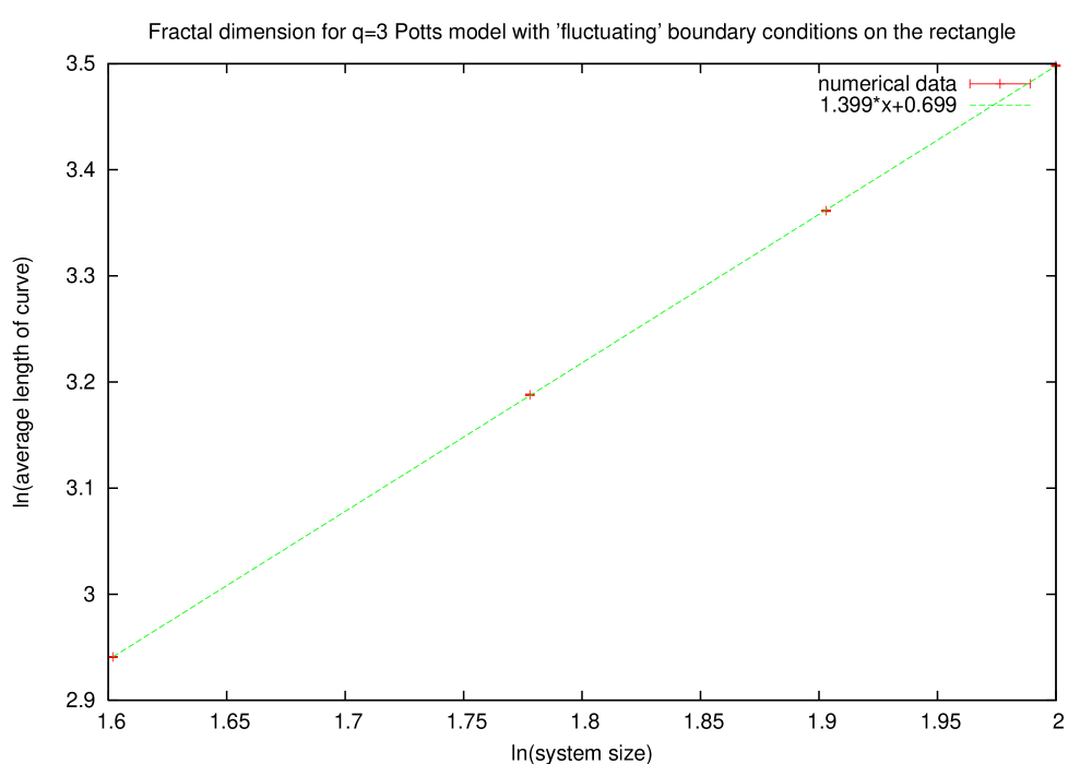
The linear fit shows the fractal dimension to be $d_{f}=1.399\pm 0.002$, which would correspond to SLE with $\kappa=3.192\pm 0.02$.

Figure 10: Schramm’s formula for $q=3$ on the rectangle for system size $100\times 300$. The distance across the sample is from the fluctuating boundary toward the spin $1$ boundary.

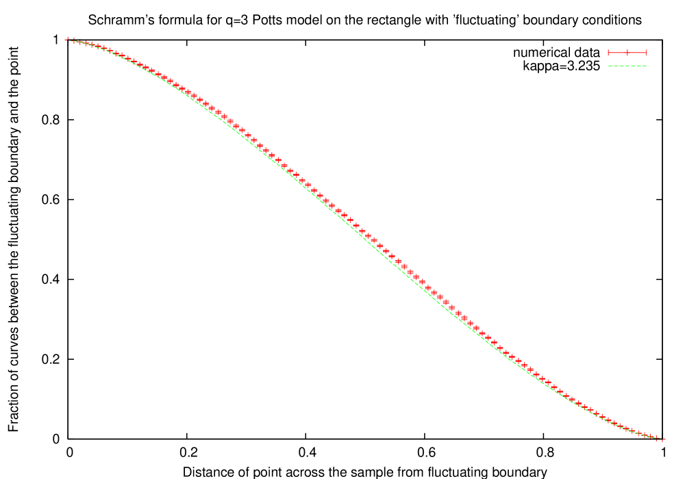
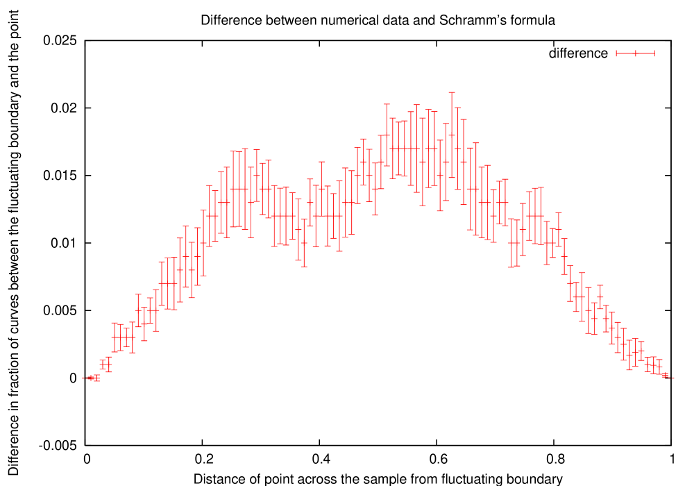
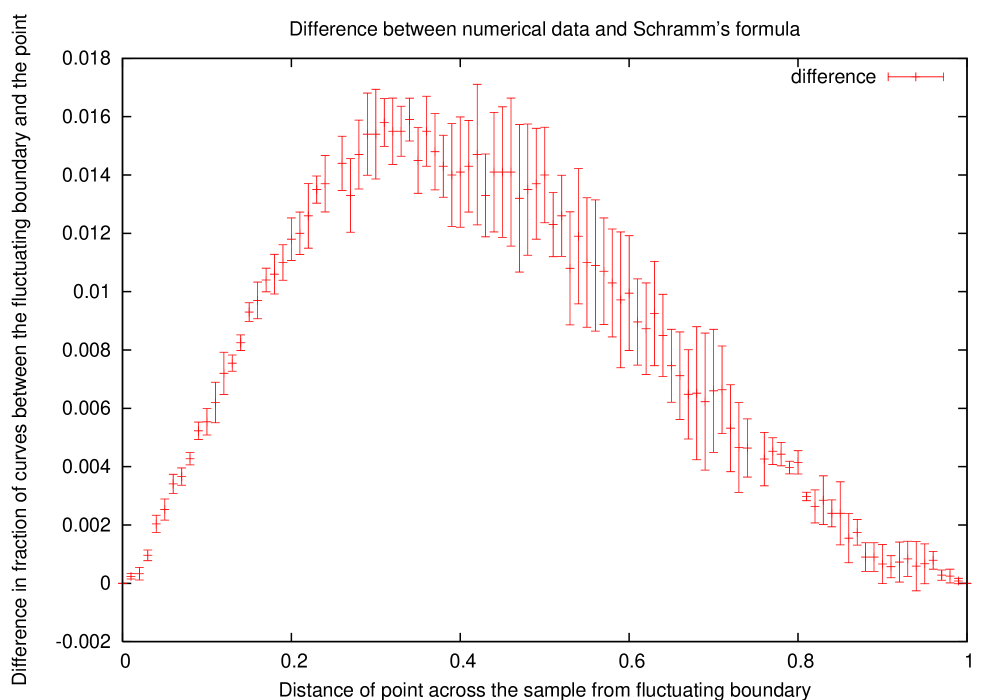
The fit to Schramm’s formula, figure 10, shows that on average, the curve is closer to the fluctuating spins boundary than would be expected. Equivalently, a point of fractional distance $0\leq s\leq 1$ across the sample from the fluctuating boundary towards the fixed boundary is more likely to be connected to the fixed spin cluster than would be expected from Schramm’s formula. Perhaps this is not surprising; whereas the two types of boundary conditions in the Ising model are reflection symmetric, the boundary conditions for $q=3$ with fluctuating boundary conditions are not. It is only in the scaling limit that we might expect to recover reflection symmetry. The best fit value is $\kappa=3.235\pm 0.01$. We shall see that this asymmetry is a result of non-zero average of the driving function, but that this effect is localised to the neighbourhood of the boundary spins, and therefore is unimportant in the scaling limit.

An alternative set of boundary conditions are the ‘fluctuating’ boundary conditions described in section 2. These lead to the existence of two cluster boundary curves; the boundary of the cluster containing one set of boundary spins and the boundary of the cluster containing the other boundary spins. Wherever the two curves overlap, this is labelled a ‘composite’ part of the curve. Where they are distinct they are labelled ‘split’ curves. In order to ascertain the fractal dimensions of the two types of curves, the expected total length of the two types of curves as a function of system size is plotted, see figure 11.

Figure 11: Fractal dimension of ‘composite’ and ‘split’ boundary types for $q=3$ Potts model on the rectangle with fixed boundary conditions. The system size is the length of the smaller side of the rectangle in units of lattice spacing.

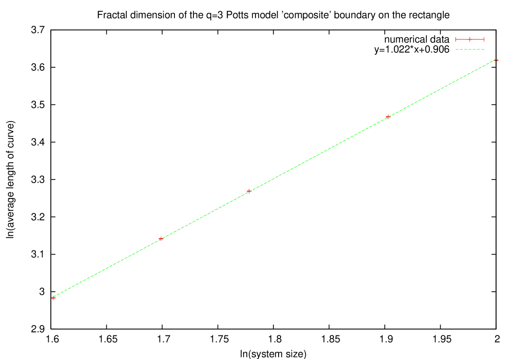
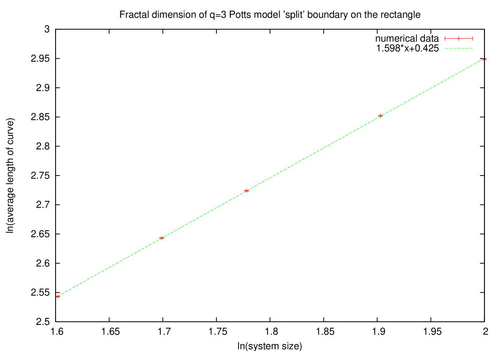
$65,000$ independent samples are generated for each sample size. The fractal dimension of the ‘composite’ boundary type is $d_{f}=1.022\pm 0.003$, which would correspond to SLE with $\kappa=0.18\pm 0.02$. The reduced $\chi^{2}$ of this linear fit is $9.7$ however, which is indicative of non-linearity in the results. Closer investigation reveals convexity resulting from the fractal dimension diminishing as system size increases. The ‘split’ boundary type has a larger fractal dimension of $d_{f}=1.598\pm 0.008$, which would result from SLE with $\kappa=4.78\pm 0.06$. This supports the hypothesis that the ‘split’ boundary types dominate in the scaling limit, resulting in a pair of curves running between the boundary points. The value of $\kappa$ is a little surprising; it is close to the dual value for $\kappa=10/3$, namely $\kappa^{\prime}=16/\kappa=4.8$.

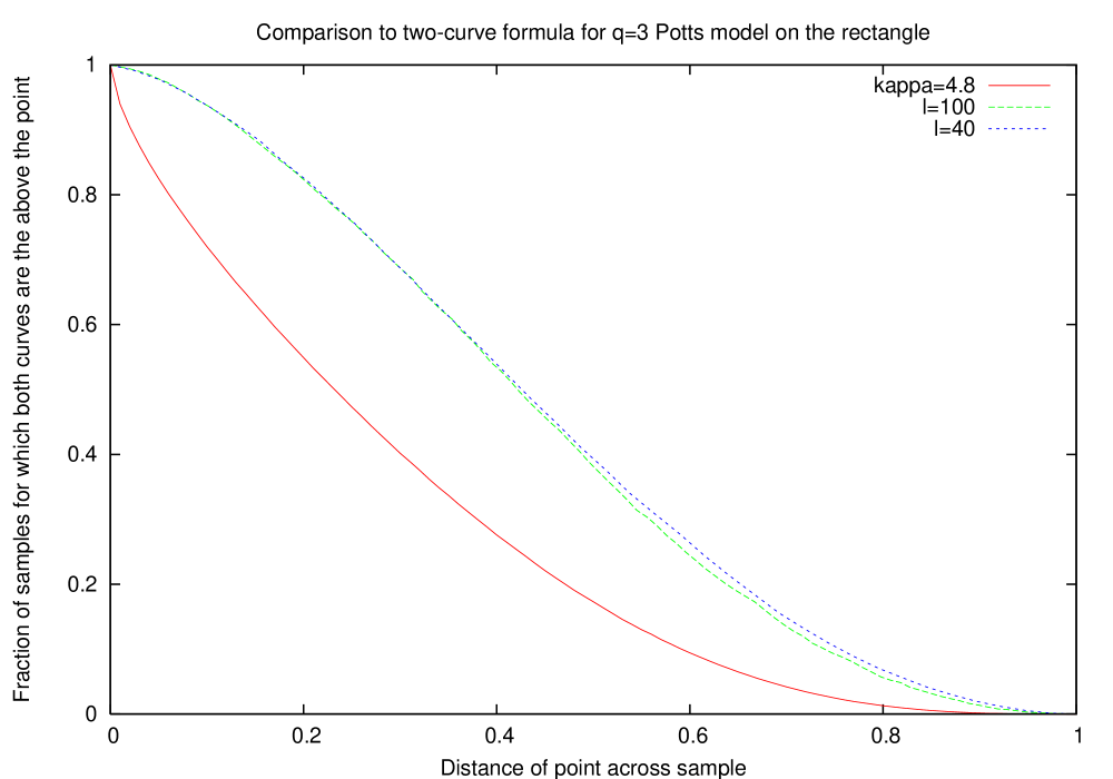
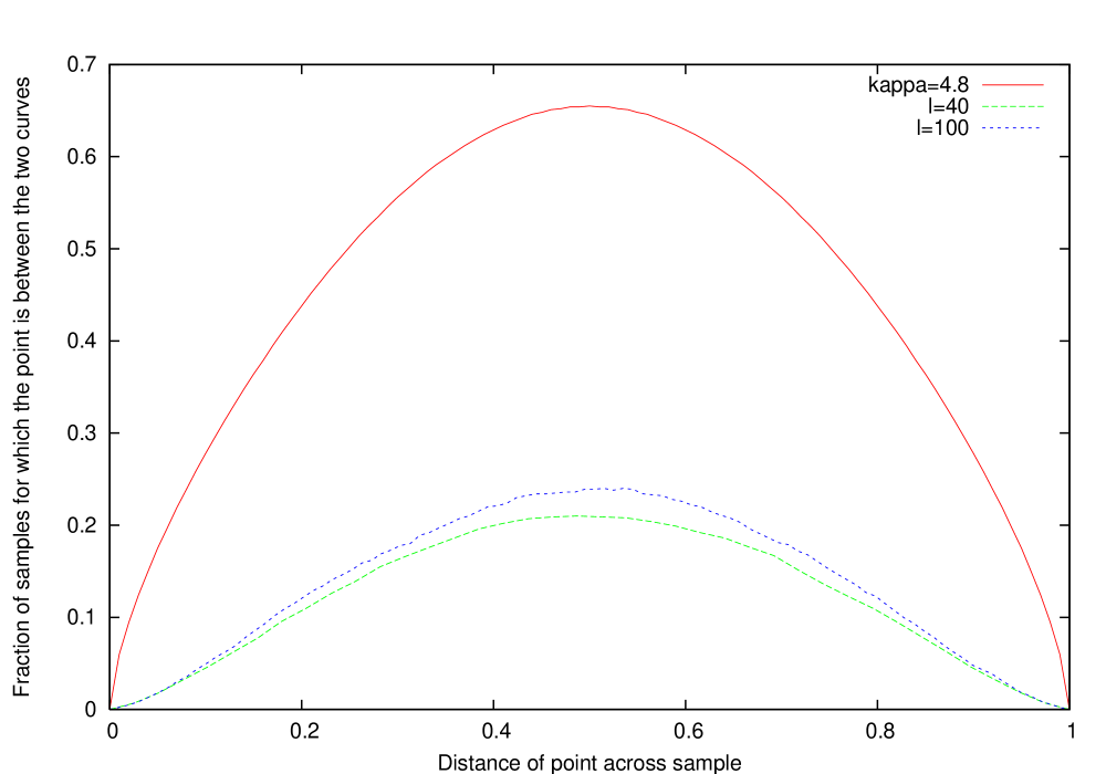
Figure 12 shows the agreement with the generalisation of Schramm’s formula to two curves, again from $65,000$ independent samples. The path used is the same as for the single curve case, namely the dashed line in figure 6. As a function of the distance of a point upwards from the bottom boundary, we may determine the expected fraction of the samples for which both cluster boundary curves are above the point (top figure) and the fraction for which the point is between the two curves (bottom figure). The fit to the two-curve formula is poor for the lattice sizes considered, as may have expected; for finite lattice size, there is a non-zero contribution from ‘composite’ cluster boundaries, which reduce the proportion of points which lie between the two curves and increase the proportion of points to one side of both curves as a result.

Figure 12: Comparison to the two-curve formula for the three-state Potts model on the rectangle. The agreement with the prediction of $\kappa=4.8$ from the fractal dimension is poor. Two system sizes are shown, $l=40$ and $l=100$, where $l$ is the smaller of the sides of the rectangle.

5.3 Ising model on the disc

The spins lie on the triangular lattice so that each spin has six nearest neighbours and the spin boundaries lie on the edges of the honeycomb lattice (the sides of the hexagons). Initially, four system sizes are considered, characterised by the maximum number of rows across the central vertical diameter: $101$, $153$, $201$ and $253$. Spins are included if the centre of the hexagon is a distance away from the centre of less than or equal to the radius of this vertical column. The geometry is shown in figure 13 with the boundary conditions used for the Ising model.

Figure 13: The geometry for the Ising model on the disc. The figure would be classified as size $13$ as this is the number of spins across the largest vertical diameter. Boundary spins are fixed as shown and bulk spins left grey. The path used for the comparison to Schramm’s formula is shown as the dashed cyan line.

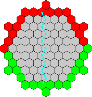
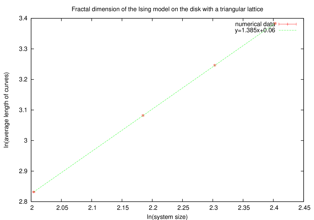
The fractal dimension of the curve in this geometry is $d_{f}=1.38\pm 0.002$, which would correspond to SLE with $\kappa=3.08\pm 0.02$, see figure 14. This result is obtained from $10,000$ independent samples for each system size.

Figure 14: The fractal dimension of the Ising model on the disc with a triangular lattice from $10,000$ samples of each system size. The size of the system is the number of spins across the central vertical diameter.

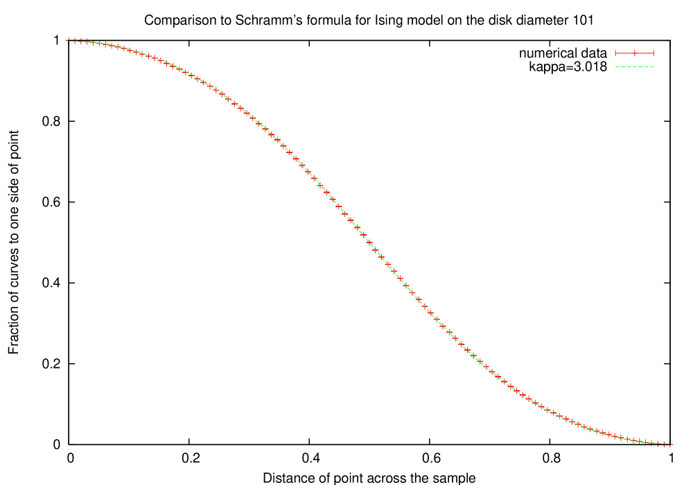
The fit to Schramm’s formula is via the Mobius transformation from the upper half plane to the disc

$$r(z)=-\frac{z-i}{z+i}\,.$$ (14)

The value of $t$ in equation 7 is related to the fractional distance $0\leq s\leq 1$ upwards along the vertical diameter by the formula

$$t=\frac{2s-1}{2s(1-s)}\,.$$ (15)

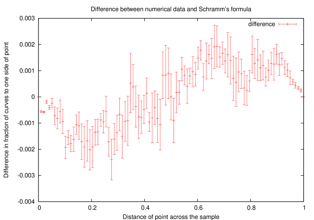
The best fit for the largest system size considered would correspond to SLE with $\kappa=3.018\pm 0.007$, as shown in figure 15. The reason that only the largest system size is shown is that the plot is quantitatively similar for all system sizes. Over the range of system sizes tested, the value of $\kappa$ fluctuates around a constant value. This appears inconsistent with the hypothesis that the value should be converging to $\kappa=3$ as system size increases, but is likely to be a result of the small range of system sizes considered. Larger systems are computationally demanding to simulate, but would offer further insight into this problem.

Figure 15: The best fit to Schramm’s formula for the Ising model on the disc with $101$ spins across the vertical diameter.. The agreement is to better than 1%, see the lower figure.

The third test against SLE is to extract driving functions for each curve and to examine their statistics as a function of system size. This process is described in section 4.4. An example, for diameter $253$, is shown in figure 16. The results are from $50,000$ independent samples. For each sample, only the part of the curve corresponding to capacity $t\leq 1/3$ was used, since the error introduced by the series of conformal maps may be expected to grow exponentially. This would result in inaccurate values for the driving function from later points on the curve.

Figure 16: The frequency of step distribution for the Ising model on the disc, diameter 253. The plot takes data from $50,000$ independent samples. The y-scale is an arbitrary measure of frequency.

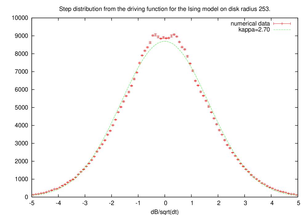
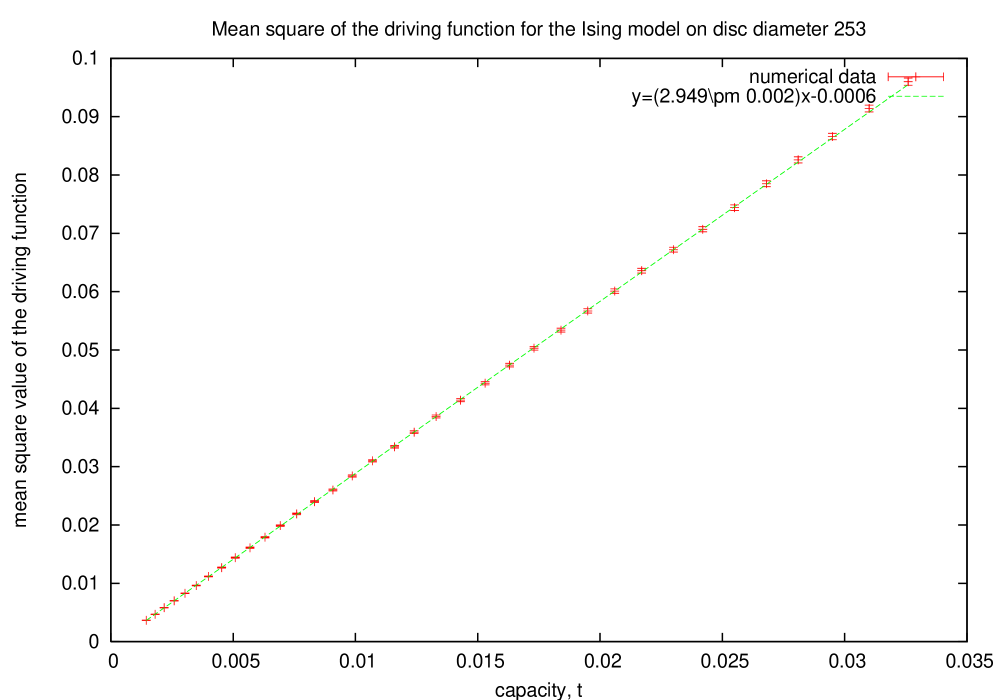
The form should be Gaussian, but the finite lattice is apparently responsible for a bi-modality for small steps $\delta B_{t}/\sqrt{\delta t}$. A second test is to examine the expected squared value of the driving function as a function of capacity, $t$. Each system size has a linear fit with a gradient which would correspond to $\kappa$. The results for diameter $253$ is shown in figure 17. The linear fit is excellent, with reduced $\chi^{2}=0.01$.

Figure 17: The expected value of $a_{t}^{2}$ plotted against capacity, $t$, for the Ising model on the disc diameter $253$. The fit is excellent, with reduced $\chi^{2}=0.01$. The data comes from $40,000$ independent samples.

The value of this best fit as a function of the inverse system size is plotted in figure 18. The approach to the scaling limit appears to be complicated; it is not a simple power law at these lattice sizes.

Figure 18: The mean gradient of the linear fit of $a_{t}^{2}$ to $t$ for the Ising model as a function of system size. The fit shown is linear, which is clearly inadequate; the approach to the scaling limit is not a simple power law at these scales.

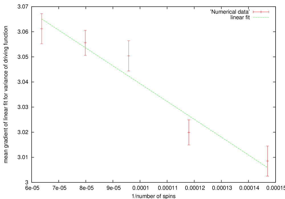
Smaller system sizes and larger numbers of independent samples are used for this test, as large numbers of samples are required to obtain results to a desirable accuracy. The table below shows the system sizes used, with the corresponding values of the inverse number of spins and number of samples generated.

System size	Inverse number of spins	Number of samples used
101	$1.47\times 10^{-4}$	760,000
113	$1.18\times 10^{-4}$	920,000
125	$9.58\times 10^{-5}$	720,000
137	$7.98\times 10^{-5}$	1,040,000
153	$6.37\times 10^{-5}$	580,000

5.4 $q=3$ Potts model on the disc

Firstly, we examine the case of ‘fluctuating’ boundary conditions, such that a single cluster boundary propagates through each sample. System sizes are again characterised by the number of spins along the central vertical diameter. System sizes considered are $101$, $153$, $201$ and $253$. The fractal dimension, obtained as usual by determining the expected curve length as a function of system size, is plotted in figure 19.

Figure 19: The fractal dimension of the $q=3$ Potts model on the disc. System size is the number of spins across the central vertical diameter.

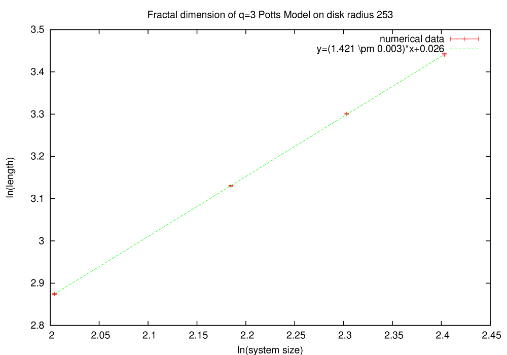
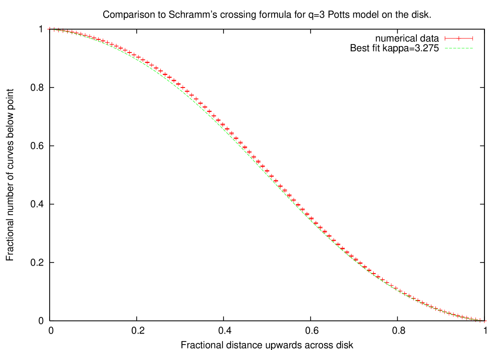
The value for the fractal dimension obtained is $d_{f}=1.4216\pm 0.0007$, which would correspond to SLE with $\kappa=3.373\pm 0.006$. This comes from considering $10,000$ independent samples of each system size. The fit to Schramm’s formula, as for the Ising model, fluctuates with system size across the range of sample sizes considered. For the largest system size considered, the best fit is to the predictions from SLE with $\kappa=3.275\pm 0.003$. This is shown in figure 20.

Figure 20: Best fit to Schramm’s formula for the $q=3$ Potts model on the disc diameter $101$. The same asymmetry is seen as for the model on the rectangle.

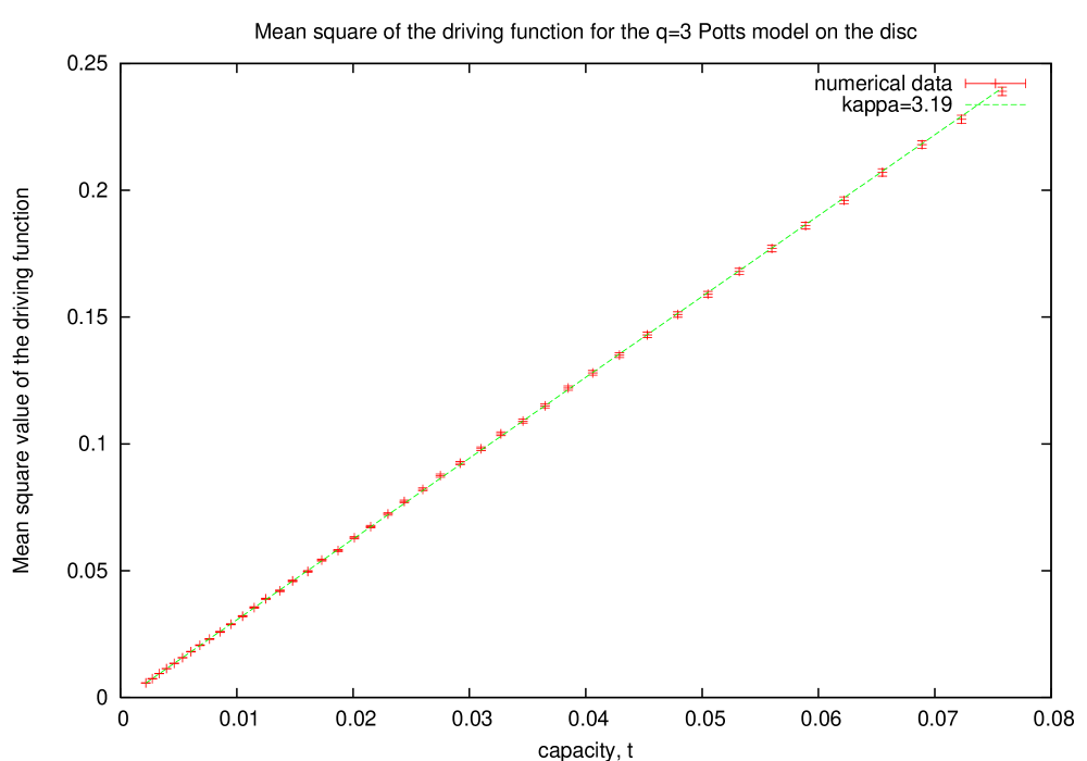
The driving function may be obtained by considering the series of conformal maps which undo the curve up to capacity, $t$, as for the Ising model in the previous subsection. A similar agreement with a Gaussian fit is again seen, with the same characteristic bi-modal behaviour at small $\delta B_{t}/\sqrt{\delta t}$. It is more instructive to examine $\langle B_{t}^{2}\rangle$ as a function of $t$ (the variance of the distribution) and to extract the gradient of the linear fit. Each system size shows linear behaviour to a high degree of accuracy. A typical plot is as in figure 21, which has reduced $\chi^{2}=0.01$.

Figure 21: The mean square value of the driving function as a function of capacity, $t$. The system is the disc of diameter $201$ and $40,000$ independent samples are used. Agreement with the linear fit is excellent.

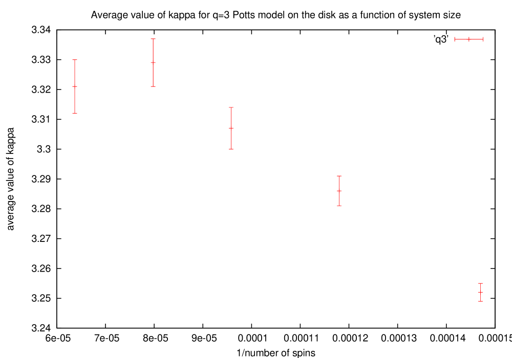
The values of the gradient of the linear fit to $\langle a_{t}^{2}\rangle$ against capacity, as a function of inverse system size, is shown in figure 22. As for the Ising model, smaller system sizes are used for this test because large number of independent samples are required to keep the error manageable. As for the Ising model, the system does not show a power law approach to the scaling limit at these system sizes.

System size	Inverse number of spins	Number of samples used
101	$1.47\times 10^{-4}$	800,000
113	$1.18\times 10^{-4}$	800,000
125	$9.58\times 10^{-5}$	800,000
137	$7.98\times 10^{-5}$	640,000
153	$6.37\times 10^{-5}$	720,000

Figure 22: The gradient of the linear fit to the mean square value of the driving function against capacity, plotted against inverse system size. The approach to the scaling limit is not a simple power law.

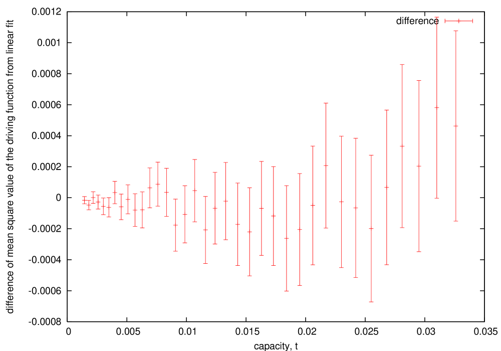
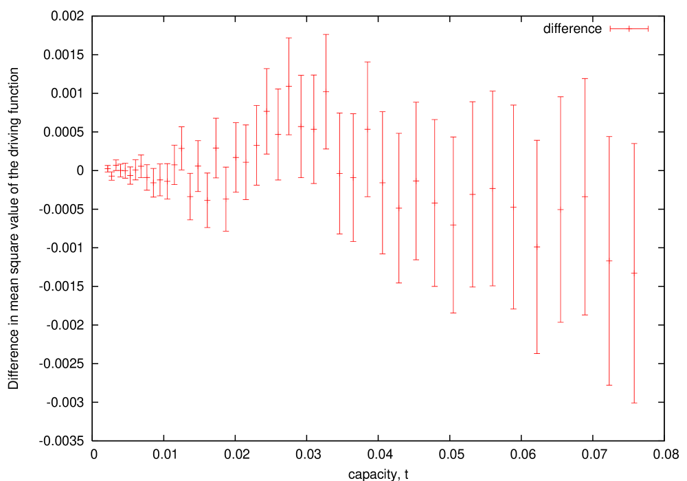
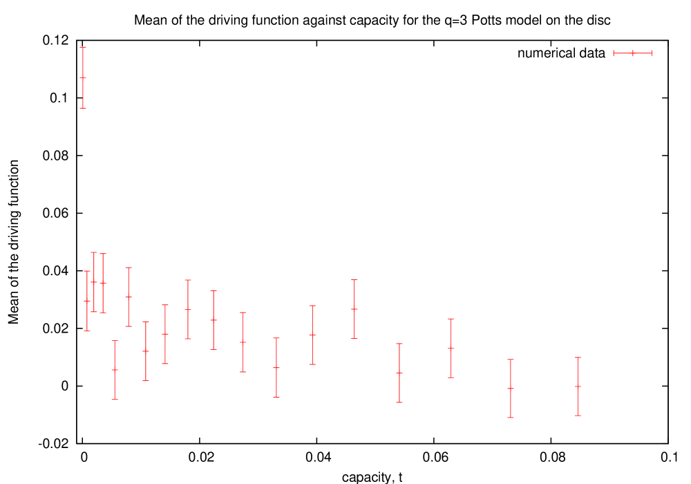
Recall that, by comparison to the fit to Schramm’s formula, the spin boundary curve of the $q=3$ Potts model with ‘fluctuating’ boundary conditions displays asymmetry. The curve is more likely to pass close to the fluctuating boundary than is predicted by SLE. This asymmetry is not surprising; the boundary conditions are not reflection symmetric, as they are in the Ising model. However, this asymmetry must vanish in the scaling limit if the curve is to become SLE. Figure 23 shows the mean of the driving function for the curve on the disc of diameter $253$ as a function of capacity, $t$. It is clear that the asymmetry is a result of the behaviour of the curve at small $t$. This is encouraging, since it suggests that this is a boundary effect, whose contribution would therefore become irrelevant in the scaling limit.

Figure 23: Mean of the driving function as a function of capacity for the $q=3$ Potts model on the disc diameter 253.

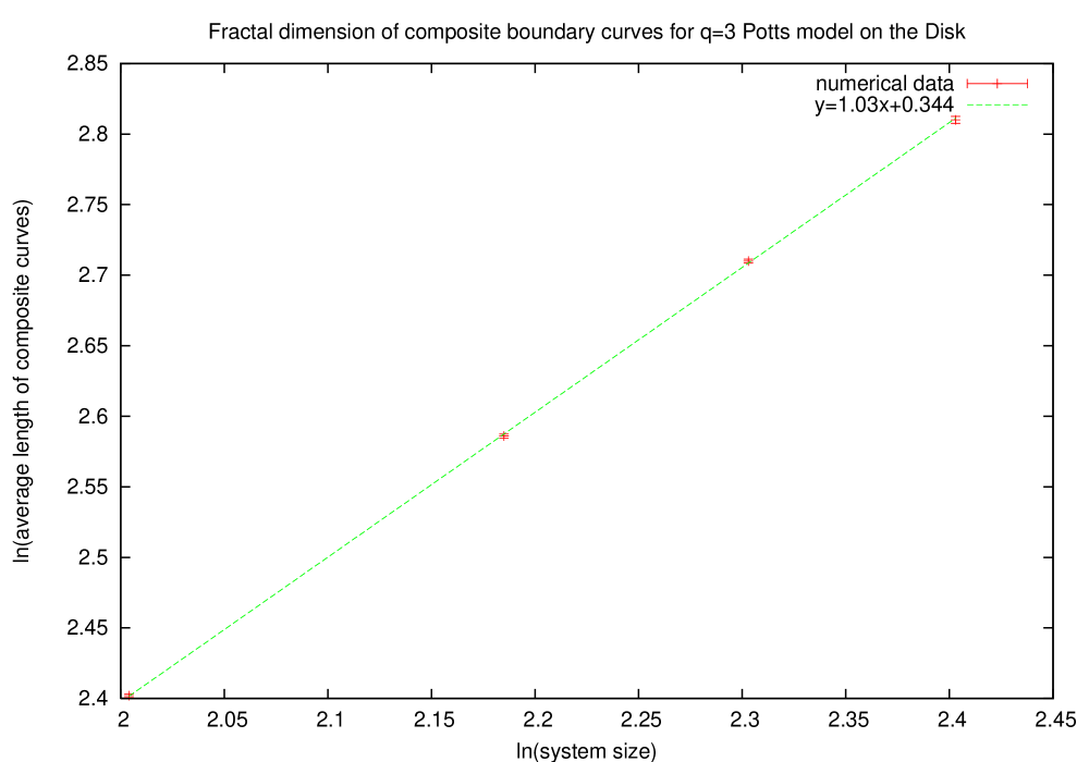
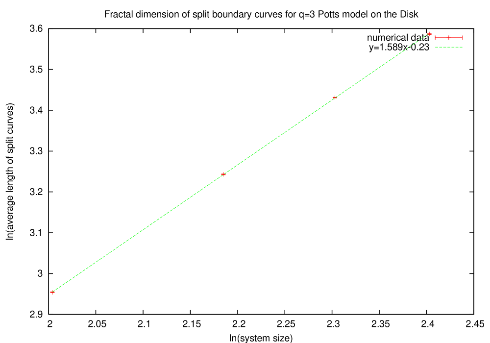
The case of ‘fixed’ boundary conditions may be tested for fractal dimension of the two types of boundary, the ‘composite’ and ‘split’ boundaries. A plot of the fractal dimension of each of these is shown in figure 24. $40,000$ independent samples of each system size were used. The fractal dimension of ‘composite’ curves is not constant but diminishing as system size increases, just as was seen for the model on the rectangle. The fractal dimension of the ‘split’ curves $d_{f}=1.589\pm 0.005$ would correspond to SLE with $\kappa=4.71\pm 0.04$. The fractal dimension of the the ‘composite’ curves is $d_{f}=1.03\pm 0.01$ ($\kappa=0.24\pm 0.08$).

Figure 24: The fractal dimensions of the ‘composite’ (top figure) and ‘split’ (bottom figure) boundaries for the $q=3$ Potts model on the disc.

6 Summary and Conclusions

Recall our hypothesis, that the scaling limit of spin cluster boundaries in the three-state Potts model is SLE with $\kappa=10/3$. The numerical results from the simulations with ‘fluctuating’ boundary conditions, and hence with single curves propagating across the samples, shows encouraging support for this hypothesis. The data should be compared to that from the Ising model, which has been proven to correspond to $SLE_{3}$. The results are summarised in the table below for the tests of the fractal dimension and best fit to Schramm’s formula, both on the rectangle and the disc.

Rectangle	Ising	$q=3$
Fractal dimension	$2.976\pm 0.02$	$3.192\pm 0.02$
Schramm’s formula	$3.02\pm 0.02$	$3.235\pm 0.01$

disc	Ising	$q=3$
Fractal dimension	$3.08\pm 0.02$	$3.373\pm 0.006$
Schramm’s formula	$3.018\pm 0.007$	$3.275\pm 0.003$

The value for the fractal dimension is the more robust result, since it incorporates data from the whole range of system sizes. Notice that the known value of $\kappa=3$ lies just outside the range obtained from the fractal dimension of the numerical simulations on the rectangle. The values obtained are a little too low for the Ising model, but also for the three-state Potts model, compared to our prediction of $\kappa=10/3$. However, on the disc, the Ising model shows a fractal dimension which is larger than the known value. In this case, the fractal dimension of the Potts model is also larger than our prediction. Qualitative agreement with Schramm’s formula for a single system size ($100\times 300$ on the rectangle and diameter $253$ on the disc) is also encouraging. We have demonstrated that the asymmetry of the curve (it is more likely to be close to the fluctuating boundary than the prediction from SLE) is a result of the behaviour of the curve at small capacity, as may be seen from a plot of the mean of the driving function against capacity. This asymmetry may be assumed, therefore, to be a boundary effect, which would be irrelevant in the scaling limit. This infers that reflection symmetry is recovered in the scaling limit, consistent with the curves being SLE.

Since the results from the variance of the driving functions do not appear to approach the scaling limit as a simple power law, it is not clear how to extract a value for $\kappa$ from the data. If we simply average over the values obtained from all system sizes considered, we find $\kappa=3.04$ for the Ising model and $\kappa=3.30$ for the $q=3$ Potts model. This figure is, of course, an arbitrary one and is supposed only to give a guide to the order of magnitude of the variance in the scaling limit. The fact that this figure is close to the predicted value is, however, encouraging.

We also considered the three-state Potts model with fixed boundary conditions, which leads to a pair of cluster boundaries, coinciding in some places. The results for $\kappa$ from the fractal dimension of these two curve types on the rectangle and the disc are summarised below.

2 Curves	Composite	Split
Rectangle	$0.18\pm 0.02$	$4.78\pm 0.06$
disc	$0.24\pm 0.08$	$4.71\pm 0.04$

The ‘split’ boundaries have a larger fractal dimension. This is consistent with the hypothesis that they dominate in the scaling limit, supported by the irrelevance of the 4-leg operator. For the sample sizes considered, the agreement with the two-curve formula (the generalisation of Schramm’s formula to two-curve SLE) is poor. This is unsurprising, as the presence of ‘composite’ cluster boundaries reduces the frequency of points being between the two curves and redistributes this to the probability that a point is to one side of ‘both’ curves.

Acknowledgements: The authors would like to thank Benjamin Doyon, Tom Kennedy, Valentina Riva, Federico Camia and David Wilson for helpful discussions and encouragement. This work was supported in part by EPSRC Grants GR/R87712/01 and EP/D050952/1. It was carried out in part at the program on ‘Stochastic Geometry’ at the Kavli Institute for Theoretical Physics, whose hospitality is gratefully acknowledged.

Appendix A The Fortuin-Kastelyn cluster representation

There exists a well known mapping of the partition function to a cluster model, which will be referred to in the appendix describing the Wolff algorithm. Up to a multiplicative factor, the partition function is

$$Z=\textrm{Tr}\prod_{r,r^{\prime}}(1-p+p\delta_{s(r),s(r^{\prime})})\,,$$ (16)

with $e^{-\beta J}=1-p$. The product may be expanded into a sum of $2^{N}$ terms ($N$ is the number of nearest neighbours) by choosing either $(1-p)$ or $p\delta_{s(r),s(r^{\prime})}$ from each bracket. If a line is drawn on the edge between each pair of spins for which the term $p\delta_{s(r),s(r^{\prime})}$ was chosen, the partition function is seen to correspond to a sum over all graphs on the edges of the original lattice. The spins in each connected cluster are constrained to take the same value, so taking the trace leads to

$$Z=\sum_{G}p^{|G|}(1-p)^{|\overline{G}|}Q^{||G||}\,.$$ (17)

The sum is over all graphs, $|G|$ is the number of edges in a given graph, $|\overline{G}|$ is the number in the complement and $||G||$ is the number of connected components, known as Fortuin-Kastelyn (FK) clusters.

Appendix B The Wolff algorithm

The Monte Carlo algorithm used throughout to generate samples was the Wolff algorithm [10, 9]. It is a Monte Carlo algorithm with the following update procedure:

1. Pick a lattice site at random.

2. Visit all neighbouring sites, adding them to the cluster with a probability $p$ if the spin is of the same type.

3. Repeat step (2) for all the newly included sites, adding their neighbours with the same probability if they are also of the same type.

4. Repeat (3) until no new sites may be added.

5. Change all spins in the cluster to a randomly chosen new spin type.

There is always a sequence of single spin flips from any configuration to any other. The probability, $p$, is related to the reduced coupling by (cf equation 16)

$$p=\frac{e^{\beta J}-1}{e^{\beta J}}\,.$$ (18)

It is the conditional probability that two neighbouring spins of the same type belong to the same FK cluster. The algorithm is therefore equivalent to isolating a single FK cluster and changing all included spins to a new type. The benefit of using this algorithm is that the phenomenon of critical slowing down is eliminated. However, the average computational time required for an update increases as the critical temperature is approached due to increasing average cluster sizes.

This procedure describes a single update. To generate a sample, we start with a random initial configurations of spins which are consistent with the boundary conditions. Then the update algorithm is run a sufficient number of times for the energy of the system to equilibriate. In this way, we arrive at the first sample. To calculate the number of updates required to produce a second, independent sample, we examine the autocorrelation function:

$$G(t_{j})=\frac{1}{t_{i}}\sum_{t_{i}}{(s_{1}(t_{i})-\langle s_{1}\rangle)(s_{1}(t_{i}+t_{j})-\langle s_{1}\rangle)}\,,\ \textrm{with}\ s_{1}=\sum_{i}{\delta_{s_{i},1}}\,,$$

for a number of samples such that the average over $t_{i}$ yields convergent results for large enough $t_{j}$. Note that $\langle s_{1}\rangle$ is also a time average. This autocorrelation function decays exponentially as $G(t_{j})\sim e^{-t_{j}/\tau}$. The correlation time, $\tau$, is a function of system size. Samples are deemed independent after 3 correlation times.

In this paper, we consider two boundary types. The first is fixed to spin type 1 (say). If a cluster generated by the Wolff algorithm connects with such a boundary, we do not flip the spins. That is to say we ignore step (5), thus keeping the boundary spins fixed to the only allowed type. The other choice of boundary condition considered is for the spins not to be allowed to be spin type 1 (say). If a cluster generated by the algorithm connects with a boundary of this type, then the allowed spin flips in step (5) of the algorithm are constrained to not be spin type 1. In this way, the boundary spins fluctuate with the sample, but never take the value 1.

References

- [1] Bauer M and Bernard D, 2D growth processes: SLE and Loewner chains, 2006 Phys. Rept. 432, 115-221 [math-ph/0602049]
- [2] Cardy J, Boundary conditions, fusion rules and the Verlinde formula, 1989, Nucl. Phys. B 324 581
- [3] Cardy J, SLE for Theoretical Physicists, 2005 Annals of Physics 318 81 [cond-mat/0503313]
- [4] Fortuin C and Kasteleyn P, On the random-cluster model, 1972, Physica 57 536
- [5] Gamsa A and Cardy J, The scaling limit of two cluster boundaries in critical lattice models, 2005, J. Stat. Mech. P12009 [math-ph/0509004]
- [6] Saleur H and Bauer M, On some relations between local height probabilities and conformal invariance, 1989, Nucl. Phys. B 320 591
- [7] Schramm O, Scaling limits of loop-erased random walks and uniform spanning trees, 2000 Israel J. Math. 118 221 [math.PR/9904022]
- [8] Smirnov S, Towards conformal invariance of 2D lattice models, 2006, Proceedings of the Inter- national Congress of Mathematicians (Madrid, August 22-30, 2006), European Mathematical Society 2 1421-1451
- [9] Swendsen R and Wang J-S, Nonuniversal critical dynamics in Monte Carlo simulations , 1987 Phys. Rev. Lett. 58, 86-88
- [10] Wolff U, Collective Monte Carlo Updating for Spin Systems, 1989 Phys. Rev. Lett. 62, 361-364
- [11] Wu F, The Potts model , 1982, Rev. Mod. Phys. 54 235 - 268