Roughness of undoped graphene and its short-range induced gauge field

Abstract

We present both numerical and analytical study of graphene roughness with a crystal structure including $500\times 500$ atoms. The roughness can effectively result in a random gauge field and has important consequences for its electronic structure. Our results show that its height fluctuations in small scales have scaling behavior with a temperature dependent roughness exponent in the interval of $0.6<\chi<0.7$. The correlation function of height fluctuations depends upon temperature with characteristic length scale of $\approx 90{\AA}$ (at room temperature). We show that the correlation function of the induced gauge field has a short-range nature with correlation length of about $\simeq 2-3{\AA}$. We also treat the problem analytically by using the Martin-Siggia-Rose method. The renormalization group flows did not yield any delocalized-localized transition arising from the graphene roughness. Our results are in good agreement with recent experimental observations.

I Introduction

An isolated two dimensional (2D) sheet of carbon atoms having a simple honeycomb structure is known as graphene wallace . According to the recent detailed measurements, these 2D zero-gap semiconductors reveal new features in their electronic properties. In particular, the low-energy quasi-particles of the system can formally be described by the massless Dirac-like fermions novoselov . Doped graphene sheets are pseudo-chiral 2D Fermi liquids with abnormal effective electron-electron interaction physics yafis . From the experimental point of view, the melting temperature of thin films decreases with decreasing thickness and become unstable when their thickness reduces to a few atomic layers evens . This observation supports the theoretical prediction that states: No strictly 2D crystal can be thermodynamically stable at finite temperatures  mermin . Consequently, the expectation of not observing a free 2D material in nature lived on till the Geim’s group discovered graphene mayer . Furthermore, because of the existing coupling between bending and stretching energy modes in any 2D material, one expects to observe a measurable undulations or at least very small roughness on the graphene sheet and will reduce electronic transport in graphene and affecting its thermal conductivity novoselov ; mayer .

In this paper, we are interested in determining the temperature dependence of graphene roughness. Here roughness is defined as the variance of the height fluctuations in graphene due to temperature. Our numerical treatments suggest that its height fluctuations have a scaling behavior in small scale with a temperature dependent roughness exponent. We also determine the temperature dependence of the amplitudes of the height structure function. We show that the induced random gauge field has a short- range correlation function with correlation length $\simeq 2-3{\AA}$. Finally, we formulate a field theoretical method to investigate the electron dynamics of the undoped graphene in such a random gauge field and show that there is no disorder-induced transition from delocalized to localized states⁷. This important result is in good agreement with the experimental observation that due to the graphene roughness localization is suppressed morozov .

The rest of this paper is organized as follows. In Sec. II, we introduce an effective interaction between carbon atoms that enters the molecular dynamic simulation to model the roughness of graphene . Section III contains our numerical calculations of graphene simulation and then using the latest results calculating the $\beta$ function analytically by using the field theory of Martin-Siggia-Rose method. We finally conclude in Sec. IV with a brief summary.

II Roughness Exponent

To study and arrive at a quantitative information of a graphene surface one may consider a surface with size $L$ and define the mean height of the surface, $\overline{h}(L,\lambda)$, and its roughness, $w(L,t,\lambda)$, by the expressions like $\overline{h}(L,\lambda)=\frac{1}{L}\int_{-\frac{L}{2}}^{\frac{L}{2}}h(\bf{x},\lambda)dx$ and $w(L,t,\lambda)=(<(h-\overline{h})^{2}>)^{(\frac{1}{2})}$, respectively. The symbol $<...>$ denotes an ensemble averaging. Here, $\lambda$ is an external factor which could be temperature in this problem  sang and $t$ is the time. In the limit of large $t$, the roughness saturates and behaves as $w(L,\lambda)\sim L^{\chi(\lambda)}$. The roughness exponent, $\chi$, characterizes the self-affine geometry of the surface. The common procedure for measuring the roughness exponents of a rough surface is to use a surface structure function, $S(r)=<|h(x+r)-h(x)|^{2}>$ which depends on the length scale $\Delta x=r$. The surface structure function is equivalent to the statistics of height-height correlation function, $C(r)$, and are related by $S(r)=2w^{2}(1-C(r))$ for stationary surfaces. The second order structure function $S(r)$ scales with $r$ as $r^{\xi_{2}}$ where $\chi=\xi_{2}/2$  bara ; jafari .

The atomic structure of graphene will force us to define two scaling exponents in $x-$ (zig-zag) and $y-$ (arm-chairs) directions. The exponents can be found via the second order structure functions, $S_{x}(r_{x})=<|h(x+r_{x},y)-h(x,y)|^{2}>$ and $S_{y}(r_{y})=<|h(x,y+r_{y})-h(x,y)|^{2}>$. The different scaling exponents in the zigzag and arm-chairs directions show the anisotropic nature of the roughness in graphene. We have used the empirical inter-atomic interaction potential, i.e., carbon-carbon interaction in graphite brenner , which has in addition three-body interaction for molecular dynamics simulation of graphene sheet to investigate its morphology and its dependence of roughness exponents on temperature. The two-body potential gives a description of the formation of a chemical bond between two atoms. Moreover, the three-body potential favors structures in which the angle between two bonds is made by the same atom. Many-body effects of electron system, in average, is considered in the Brenner potential, through the bond-order and furthermore, the potential depends on the local environment.

It is well known that the harmonic approximation resulting in bending instabilities due to soft wavelength phonons leads to crumpling of a membrane. It is important to note that the Brenner potential has anharmonic coupling between bending and stretching modes which prevents crumpling. We have considered a graphene sheet including a size of $500\times 500$ atoms with periodic boundary condition. Considering the canonical ensemble (NVT), we have employed Nosé-Hoover thermostat to control temperature. Our simulation time step is $1~{}fs$ in all cases and the thermostat’s parameter is $5~{}fs$. Therefore, we have found a stable 2D graphene sheet in our simulation.

III Numerical results

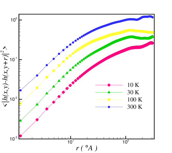
In the top graph of Fig. 1, we have shown a snapshot of the graphene fluctuations at temperature $300K$. Moreover, the magnetic field induced by the roughness is shown in the bottom graph to emphasize the randomness of the surface structure. Order of height fluctuations are about $\sim 5{\AA}$ which is in good agreement with experimental observationmayer . In Fig. 2, we have plotted (in log-log scales), the structure function in the arm-chairs direction, namely $S_{y}(r_{y})$, simulated at temperatures $10,30,100$ and $300$ $K$. Fig. 2 shows that for some characteristic length scales, the scaling behavior of the structure functions do not exist. The typical characteristic length scales are approximately $90{\AA}$ at room temperature which is in good agreement with experimental findings mayer that is in the range of $50-100{\AA}$.

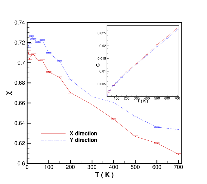
In Fig. 3, the temperature dependence of the scaling exponents, $\chi$‘s, in both zigzag and arm-chairs directions are given. As shown at low temperatures, the exponents for zigzag- and armchairs- directions are about $0.7$ (see also Ref. L ). However, the exponent for armchairs direction is greater than the one for zigzag direction at large enough temperatures. We have also used the bond order potential proposed by Ghiringhelli et al. los , and found good agreement between the results of the two potentials  Faso . This is physically understandable, since our simulation has been performed for $T<700K$ and the two potentials mainly differ at higher temperatures. Fig. 3 (inset) shows also the amplitude of the second moments, $C_{x}$ and $C_{y}$, which are defined as, $S_{x}(r_{x})=C_{x}r_{x}^{{\xi_{2}}_{x}}$ and $S_{y}(r_{y})=C_{y}r_{y}^{{\xi_{2}}_{y}}$ in the scaling region, in terms of temperature.

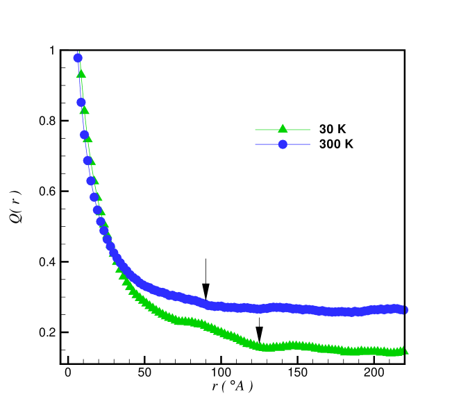
To determine the characteristic length scales, we define the quantity $Q(r)$ as the difference between the joint probability distribution function (PDF) of height fluctuations at two points. For instance, given $y$ and $y+r$ points, the $Q(r)$ is calculated by $P(h_{1},y;h_{2},y+r)$ and product of two PDFs, $P(h_{1},y)$ and $P(h_{2},y+r)$ CMB . Thus,

$$Q(r)=\int dh_{1}dh_{2}|P(h_{1},y;h_{2},y+r)-P(h_{1},y)P(h_{2},y+r)|~{}.$$ (1)

In Fig. 4 we have shown $Q(r)$ as a function of $r$. This figure clearly indicates that the height fluctuations at scales of $90{\AA}$ and $125{\AA}$ for $T=300K$ and $T=30K$, respectively, are almost independent. Obviously, the $Q(r)$ becomes $r-$ independent after these values of $r$ (by considering its error bars). Furthermore, we have found the same value for correlation length for graphene with fixed boundary condition. As a consequence, this length scale is not an artifact of boundary conditions.

IV MARTIN-SIGGIA-ROSE EFFECTIVE ACTION

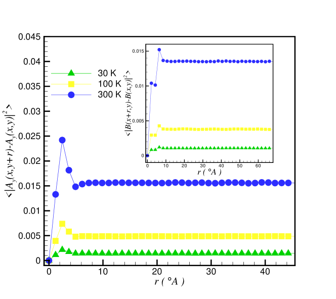
Roughness of graphene results in a random gauge field and affects its electronic structure iordanskii . The dependence of the hopping integral $\Gamma$ on the deformation tensor is expressed by $\Gamma=\Gamma_{0}+\frac{\partial\Gamma}{\partial u_{ij}}u_{ij}$, where $u_{ij}$ nelson is given by $u_{ij}=\frac{1}{2}\{\frac{\partial u_{i}}{\partial x_{j}}+\frac{\partial u_{j}}{\partial x_{i}}+\frac{\partial u_{k}}{\partial x_{i}}\frac{\partial u_{k}}{\partial x_{j}}+\frac{\partial h}{\partial x_{i}}\frac{\partial h}{\partial x_{j}}\}$. Here, $x_{i}\equiv(x,y)$ are coordinates in the plane and $u_{i}$ are the corresponding components of the displacement vector. In the presence of roughness, an effective Dirac Hamiltonian describes the electron states near the K-point, $H=v_{F}\sigma(-i\hbar\nabla-\frac{e}{c}\bf A)$, where $v_{F}=\sqrt{3}\Gamma_{0}a/2\hbar$ and $\bf A$ is the gauge field. The gauge field can be written in terms of the hopping integral $\Gamma$ as: $A_{x}=\frac{c}{2ev_{F}}(\Gamma_{2}+\Gamma_{3}-2\Gamma_{1}$ ) and $A_{y}=\frac{\sqrt{3}c}{2ev_{F}}(\Gamma_{3}-\Gamma_{2})$ katsnelson . Labels $1,2$ and $3$ refer to the nearest neighbors atoms with vectors $(-a/\sqrt{3},0),(a/2\sqrt{3},-a/2)$ and $(a/2\sqrt{3},a/2)$, respectively. In Fig. 5, we have plotted the structure function of the gauge field $\bf A$, namely $S_{A}(r)=<|(\bf A(\bf x+\bf r)-\bf A(\bf x))\cdot\hat{x}|^{2}>$ versus the scale in $y$-direction. The vectors $\bf r$ and $\hat{\bf x}$ can be chosen in $x-$ and $y-$ directions. Therefore, we have four different types of structure functions. As shown in Fig. 5, the gauge field and the related magnetic field have small scale correlation with correlation length $l_{c}\simeq 2-3{\AA}$. We have checked the other three structure functions of the induced gauge field and their cross correlation functions and find that they have small scale correlation and are almost statistically independent.

In what follows we have developed a renormalization group analysis to investigate the Dirac equation in random gauge field and show that no delocalization-localization transition occurs for electrons in such a random gauge potential^20,21.

The Lagrangian of Dirac fermions in (2+1) dimensions and in the presence of gauge potential $A_{\mu}$ is given by: ${\mathcal{L}}=i\int dt\int d^{2}{\bf x}\bar{\psi}\gamma^{\mu}(\partial_{\mu}-A_{\mu})\psi$, in which $\gamma^{0}=\sigma_{z},\gamma^{1}=i\sigma_{y},\gamma^{2}=-i\sigma_{x}$, $\sigma$’s are the Pauli matrices and $\gamma$’s satisfy the Clifford algebra $\{\gamma^{\mu},\gamma^{\nu}\}=2g^{\mu\nu}$. The wave functions $\psi(\bf x,t)$ and $\bar{\psi}(\bf x,t)$ are 2D Dirac spinors and $A_{\mu}$ is a static random gauge field with a Gaussian distribution having zero mean value. The covariance is given by $\langle(A_{i}({\bf x})A_{j}({\bf x}^{\prime})\rangle=2D_{0}\delta_{ij}\delta({\bf x}-{\bf x}^{\prime})$ where $i,j\equiv 1,2$ and $D_{0}$ is the intensity of its spatial fluctuations. This relation shows the spatially uncorrelated nature of the gauge filed. We note that the Fermi velocity of electrons in graphene is of the order of $10^{6}$ m/s and the typical velocity of the height fluctuations is of the order of $30$ m/s. Therefore, the random gauge potential will act as a quenched random field on electrons. Focusing on a single mode with energy $\epsilon$ we get the following expression for the Lagrangian:

$${}{\mathcal{L}}=\int d^{2}{\bf x}\bar{\psi}(i\gamma^{k}\partial_{k}-i\gamma^{k}A_{k}+\epsilon\gamma^{0})\psi~{}.$$ (2)

The expectation value of any operator $\mathcal{O}$ can be calculated as follows

$$\langle{\mathcal{O}}\rangle=\frac{\int{\mathcal{D}}\psi{\mathcal{D}}{\bar{\psi}}{\mathcal{O}}\exp(-i{\mathcal{L}})}{Z}~{},$$ (3)

in which $Z$ the partition function is defined by

$$Z = \int{\mathcal{D}}\psi{\mathcal{D}}{\bar{\psi}}{\mathcal{O}}\exp(\int d^{2}{\bf x}\bar{\psi}(-\gamma^{k}\partial_{k}+\gamma^{k}A_{k}-i\epsilon\gamma^{0})\psi)$$ (4)

$$= \det(-\gamma^{k}\partial_{k}+\gamma^{k}A_{k}-i\epsilon\gamma^{0})~{}.$$

Introducing the Dirac bosons $\chi$ and ${\bar{\chi}}$, one can re-expressing the above determinant as follows

$$Z^{-1}=\int{\mathcal{D}}\chi{\mathcal{D}}{\bar{\chi}}\exp\left(-\int d^{2}{\bf x}\bar{\chi}(-\gamma^{k}\partial_{k}+\gamma^{k}A_{k}-i\epsilon\gamma^{0})\chi\right),$$ (5)

and implicitly we have

$$\langle{\mathcal{O}}\rangle=\int{\mathcal{D}}\psi{\mathcal{D}}{\bar{\psi}}{\mathcal{D}}\chi{\mathcal{D}}{\bar{\chi}}{\mathcal{O}}\exp\{\int d^{2}{\bf x}\bar{\psi}(-\gamma^{k}\partial_{k}+\gamma^{k}A_{k}-i\epsilon\gamma^{0})\psi-\int d^{2}{\bf x}\bar{\chi}(-i\gamma^{k}\partial_{k}+\gamma^{k}A_{k}-i\epsilon\gamma^{0})\chi\}.$$ (6)

Now by integrating the above result over the Gaussian variable $A_{\mu}$ whose probability density function is given by

$$P\propto\exp(-\frac{1}{4D_{0}}\int d{\bf x}A_{k}^{2}),$$ (7)

one reaches the following result for the averaging of expectation values over quenched random gauge

$$\langle\langle{\mathcal{O}}\rangle\rangle=\int{\mathcal{D}}\psi{\mathcal{D}}{\bar{\psi}}{\mathcal{D}}\chi{\mathcal{D}}{\bar{\chi}}{\mathcal{O}}\exp(-S_{0}-S_{int})~{},$$ (8)

where the free part of the effective action is

$$S_{0}=\int d^{2}{\bf x}\bar{\psi}(\gamma^{k}\partial_{k}+i\epsilon\gamma^{0})\psi+\int d^{2}{\bf x}\bar{\chi}(\gamma^{k}\partial_{k}+i\epsilon\gamma^{0})\chi~{},$$ (9)

and the interaction part

$$S_{int}=-D_{0}\int d^{2}{\bf x}\left[\left({\bar{\psi}}\gamma^{k}\psi+{\bar{\chi}}\gamma^{k}\chi)\right)\cdot\left({\bar{\psi}}\gamma^{k}\psi+{\bar{\chi}}\gamma^{k}\chi\right)\right]~{},$$ (10)

where $k=1,2$. The $\beta$ function of the coupling $D_{0}$ will determine its behavior under changing the scale. We found that in one-loop order the correction to the short-range roughness intensity ($D_{0}$) is proportional to $k^{2}$ , therefore this correction vanishes in long-wave length limit. One can see that the same will happen at higher order of of perturbation, leading us to the conclusion that the vanishing of the beta function in all orders should be the consequence of the Ward identity due the conservation of Dirac current which leads to an incompressible flow of electrons in the low energy limit( $\epsilon\sim 0$).

This result shows that the resistance against the electron flow due the interaction of Dirac fermions and roughness of the Graphene, remains unchanged under renormalization group flow towards large scales, and this in turn, excludes the possibility of the localization of low energy states (For more details, see for instance Ref[morpurgo, ; morozov, ; demartino, ; aleiner, ; ziegler, ]).

V Summary

In Conclusion, we find the temperature dependence of the roughness exponents in different directions of a graphene sheet by simulating the surface within molecular dynamics approach. We have used the Brenner empirical inter-atomic interactions for graphite which is a semiconductor. The point we are making in this publication is the further detailed explanations raised in Ref.[Faso, ] which roughness could affect. We answer the question whether the roughness could lead to localized electrons in graphene or not?. The correlation function of height fluctuations shows that depending on the temperature, there are characteristic length scales in the order of $\approx 90{\AA}$ at room temperature. We show that the induced gauge field has a short- range nature with correlation lengths approximately $\simeq 2-3{\AA}$. More importantly, roughness essentially can affect to the electronic properties like conductivity and modulation of the hopping integrals castro . We treat the problem analytically by using the Martin-Siggia-Rose method. The renormalization group flows do not yield any delocalized-localized transition due to roughness. In the present work, the effect of Dirac-like electrons on roughness are not considered. It would be of intrest to develop our work may use the quantum molecular dynamics simulation or ab initio Car-Parinnello molecular dynamics for Dirac-like electrons to investigate the dependence of Dirac-like electron on the graphene roughness.

Figure 1: (color online) Snapshot of the graphene surface at $300K$ (upper graph). The sample contains a lattice size of $500\times 500$ atoms. In the lower graph, we have plotted the induced magnetic field due to the roughness of graphene surface.

Figure 2: (color online) Log-log plot of the second moment of height difference as a function of $r$, in $y$ (arm-chairs) direction, which shows that for samples with temperatures $10,30,100$ and $300$ $K$ the hight fluctuations have scaling behavior in small scales. It indicates that the roughness exponent (the slope of the plots) decreases with temperature, and means that the surface will be rough at high temperatures. A similar figure can be found for the height-height structure function in $x$ (zigzag) direction.

Figure 3: (color online) The temperature dependence of the roughness exponents show that graphene is smoother in arm-chairs direction as compared to zigzag direction. For very smooth surface the exponent will be $\sim 1.0$. At high temperature limit the exponents approach a random noise exponent (i.e. 0.5). The anisotropy of the graphene is due to the fact that the lattice spacing in arm-chairs and zigzag directions are different. It shows that (inset) the amplitude of the second moments, $C_{x}$ and $C_{y}$, are increasing function of temperature.

Figure 4: (color online)Scale dependence of $Q(r)$, defined by Eq.(1) as a function of $r$. It shows that the height fluctuations have characteristic scales of $90{\AA}$ and $125{\AA}$ for $T=300K$ and $T=30K$, respectively.

Figure 5: (color online) Log-log plot of the second moment of the induced gauge field (inset structure function of magnetic field) in $y$ direction, for samples with temperatures $30,100$ and $300$ $K$. The correlation length is about $2-3{\AA}$. Similar figures can be found for the other three gauge field structure functions.