Wang-Landau molecular dynamics technique to search for low-energy conformational space of proteins
Abstract
Multicanonical molecular dynamics (MD) is a powerful technique for sampling conformations on rugged potential surfaces such as protein. However, it is notoriously difficult to estimate the multicanonical temperature effectively. Wang and Landau developed a convenient method for estimating the density of states based on a multicanonical Monte Carlo method. In their method, the density of states is calculated autonomously during a simulation. In this paper, we develop a set of techniques to effectively apply the Wang-Landau method to MD simulations. In the multicanonical MD, the estimation of the derivative of the density of states is critical. In order to estimate it accurately, we devise two original improvements. First, the correction for the density of states is made smooth by using the Gaussian distribution obtained by a short canonical simulation. Second, an approximation is applied to the derivative, which is based on the Gaussian distribution and the multiple weighted histogram technique. A test of this method was performed with small polypeptides, Met-enkephalin and Trp-cage, and it is demonstrated that Wang-Landau MD is consistent with replica exchange MD but can sample much larger conformational space.
pacs:
02.70.Ns, 87.15.-vI Introduction
Computer simulation has been established as a technique for studying the systems with many degrees of freedom such as spin glasses and proteins. The difficulties in studying such systems stem from the fact that the conformational space is very large and there exist a huge number of local minimum energy states. For studying interesting phenomena or calculating quantities such as the transition of states or the free energy of the system, a global sampling of the conformational space and uniform sampling on energy space is desired. Canonical simulations at high temperatures realize the global sampling but low energy states are poorly sampled. At low temperatures, simulations can sample low energy states but the global search is difficult. In order to overcome these difficulties, many generalized-ensemble algorithms have been developed such as the multicanonical algorithm Berg and Neuhaus (1991) and the replica exchange method (REM) Hukushima and Nemoto (1996); Sugita and Okamoto (1999).
The multicanonical method is based on artificial weight factor by which a simulation realizes a flat energy histogram. This weight factor is not known a priori and has to be determined by iterating simulations and estimations. If the value of the weight factor is partially too large or small, then it causes to disturb a random walk in energy space. Therefore, the multicanonical weight factor needs to be fairly accurate. However, obtaining an accurate weight factor is often difficult and requires a great deal of expertise. In REM, a number of non-interacting replicas of the original system at different temperatures are simulated independently and simultaneously. Every few steps the temperatures of pairs of replicas are exchanged, subject to a detailed balance condition. As the system size increases, however, the required number of replicas also greatly increases. In such a huge simulation system, it takes an unrealistically long CPU time for a replica to traverse the entire temperature range.
Wang and Landau Wang and Landau (2001) proposed a simulation method to sample conformational space efficiently. In their method (hereafter referred to as the WL method), the weight factor is automatically estimated while the multicanonical simulation is performed. This method is originally based on a Monte Carlo (MC) algorithm.
In this paper, we focus on efficient sampling over the conformational space of an all-atom model of protein. Molecular dynamics (MD) and MC are the standard techniques for all atom protein simulations. It is recognized that the sampling efficiency of the MC method is comparable, or sometimes superior to MD for liquid simulations. In protein simulations, however, MD shows about 1.5 times better sampling efficiency Yamashita et al. (2001). This difference is attributed to the inertia force term in MD, which does not exist in MC.
Recently, MD with the WL method was applied to simulations of solutions Åberg et al. (2004) in which the original WL algorithm was applied to MD simulations in a straightforward manner. As we mention in detail later, the simple application of the WL method to MD does not work well for a protein system for a number of reasons. First, in the multicanonical MD or related methods such as the WL MD, not only the density of states but its derivative are required. In the WL method, the density of states is rugged, so that its derivative is of poor accuracy. Second, as the WL method realizes quick random walk in energy space then for a polymer such as a protein, temperature changes occur in a time scale shorter than is necessary for a change of the structure of the whole molecule. Eventually it takes a long time for a meaningful structural change to occur. In this paper, we present techniques for implementing an efficient WL MD method to circumvent these problems.
This paper is organized as follows. We describe a detailed formulation of the Wang-Landau molecular dynamics (WLMD) method in Sec. II. In Sec. III, we introduce the model system for the present study, the Met-enkephalin, a 5-residue peptide, and the Trp-cage, a 20-residue protein. Next, we compare the sampling efficiency of the current method with that of the replica exchange MD (REMD) method in Sec. IV.
II Method
II.1 The Wang-Landau method
Wang and Landau have developed a very powerful MC simulation technique for efficiently sampling conformational space. In their method, the transition probability from energy to is given by
| (1) |
where is the density of states. This is the same as in the standard multicanonical MC method. Since is not known a priori, one has to determine it by some means. In conventional multicanonical simulations, it is determined by iterating short preliminary simulations using
| (2) |
where and are the density of states and the histogram in the th simulation, respectively, and is a set of allowed energy levels. What is unique of the WL method resides in the scheme for updating . When an energy level, , is visited at the time step, , the existing is modified by a modification factor , i. e.,
| (3) |
For a given energy, , if is smaller than the true density of state, , the energy state is sampled intensively so that is updated to approach the true value, . On the contrary, if , the sampling of the energy state, , is suppressed and other energy states are extensively sampled. Although is unknown at the very beginning of simulation, approaches the true value quickly and automatically. Since is updated every step, it is possible for the system to escape local minima in a very short period of time.
II.2 The Wang-Landau molecular dynamics
We apply the WL method to MD simulations. The equation of motion for the multicanonical MD is given by Hansmann et al. (1996); Nakajima et al. (1997)
| (4) | |||||
| (5) |
where , , and represent mass, velocity, and coordinate of th atom, and the inverse temperature, ( is the Boltzmann constant), with the simulation temperature, . is referred to as the multicanonical temperature. In a straightforward application of the WL method to MD, the density of states, , could be estimated according to Eq. (3). However, such a simple method does not work well in practice. It is necessary to accurately estimate not only but also its derivative . In numerical calculation, is divided into bins, and each bin is given a discrete value. In general, the estimate of is of low accuracy due to the ruggedness between neighboring bins. In order to smooth this ruggedness, we approximate canonical energy distribution at various temperatures by the Gaussian distribution and combine them with the weighted histogram method (WHAM) Kumar et al. (1992) for updating and estimating the multicanonical temperature.
In the canonical ensemble at an inverse temperature, , the distribution of energy is written as
| (6) |
where is the density of states and
| (7) |
The last equation [Eq. (7)] defines the partition function. The canonical distribution usually has a bell-like shape. At the energy corresponding to the peak of the distribution, the equation is satisfied. This is rewritten as
| (8) |
By comparing Eqs. (5) and (8), one can see that the multicanonical temperature at energy is the temperature of a canonical ensemble whose peak energy is . If and are known, it is possible to solve Eq. (8) for . However, it is difficult to evaluate since is inaccurate if is estimated from a simulation (which is the case in practice). On the other hand, it is relatively easy to estimate the thermal average as
| (9) |
where is the density of states estimated from the simulation. The variance of the energy can be estimated in the same manner,
| (10) |
Hansmann Hansmann (1997) suggested using instead of . In his prescription, is determined from the table of . The canonical distribution of the systems that we are interested in is similar to the Gaussian distribution. Using and the deviation at , we assume that the following approximation holds:
| (11) |
which can be rearranged, using Eqs. (6) and (11), to
| (12) |
It is possible to calculate the right-hand side from a canonical simulation, but the accuracy decrease as increases. In order to keep the accuracy for a wide energy range, is estimated by using the WHAM technique with a number of temperatures,
| (13) |
where
| (14) |
and ’s are appropriate weight factors (see below). and can be obtained by solving Eqs. (13) and (14) iteratively. From Eqs. (11) and (13), it follows that
| (15) |
which can be further reduced, by using Eq. (6), to
| (16) |
Both and vanish in this expression. We use this equation for estimating the multicanonical temperatures. Note that Eq. (11) is not exact. This implies that our method may not be suitable for a system with doubly peaked distribution, for example. Nevertheless, such an error should be small if we use a sufficiently large number of temperatures.
In a WLMD simulation, we need to specify the lowest and highest temperatures for the system ( and , respectively),
and prepare energy bins and temperatures corresponding to each energy bin.
The initial estimate of the density of states, , is obtained as
follows.
We first run a short (say, 100 steps) canonical MD simulation at the inverse temperature (corresponding to the highest temperature),
and calculate the average and variance of the energy from this short simulation.
We then apply Eqs. (12) and (7) iteratively, which
yields the initial estimate .
The rest of a WLMD proceeds as follows.
(1) Set and .
(2) A canonical MD is performed for a very short period of time (say, 100 steps) according to Eq. (5) with fixed . During this period, the time average and the variance of the energy are estimated. The Gaussian energy distribution based on these values is denoted . Let the energy value of the last step of this canonical simulation be . Let and .
(3) The average and variance of energy at the inverse temperature are estimated using all the energy values that have been visited with up to this time step. Using these values, the Gaussian distribution is obtained. Similarly, the Gaussian distribution at , , is estimated. is set to zero if the simulation has never visited this temperature.
(4) For each energy bin, , calculate the corresponding temperature according to Eq. (16) with the Gaussians , , , and . The weight is set to 1 except for for which the weight is set to a specified modification factor [this factor corresponds to in Eq. (3)]. (Note that, for , is not yet defined and is set to zero.)
(5) Using the temperatures obtained in the previous step, calculate, from Eqs. (9) and (10) as well as the current estimate of the density of states , the average and variance, and , and the Gaussian distribution, .
(6) Iterate steps 4 and 5 until all the ’s converge.
(7) Update the density of states using Eqs. (13) and (14) and the Gaussians to obtain the next estimate .
(8) Estimate the next multicanonical temperature according to Eq. (16) at the energy of the last canonical MD step, . If or , is evaluated at or , respectively. This is necessary for a stable simulation.
(9) Set and go back to step 2.
In order to avoid numerical overflow in the calculation of in the step 7, we limit the summation in Eq. (13) to those inverse temperatures satisfying
| (17) |
Recently, Kim et al. Kim et al. (2003) developed the method to determine the multicanonical temperature automatically. The notable points in their method are the short period update and adding the derivative of histogram to the multicanonical temperature. While their method is different from our method in the way to update the histogram, the idea of the short term update is common. They use the finite difference of raw data (energy histogram) for update. Since the present method uses the Gaussian mask and the WHAM technique to estimate the density of states and its derivative, it is expected to be more robust.
II.3 Separation of bond and non-bond interaction
When we first applied the above method to a protein system, a random walk in the energy space was readily realized. However, the protein conformation changed very little in the whole process. It was found that the energy change predominantly originated from the bond length and the bond angle deviations. As a result, the bond energy almost solely contributed to . To avoid this artifact, we separated the bond interaction from the non-bond interaction, and applied the multicanonical ensemble only to the non-bond interaction. The energies of bond and non-bond interactions are written as and , respectively, i. e.,
| (18) |
Using and , density of state is represented as . The equations of motion with the is now expressed as
| (19) |
with
| (20) | |||||
| (21) |
Then it is possible to give different temperatures for bond and non-bond interactions. In order to suppress the motion due to the bond interaction and to facilitate global conformational changes, is fixed whereas is varied according to the WLMD scheme from a low to high temperature.
III Model for Numerical Calculation
We carried out simulations using a customized version of the PRESTO molecular simulation package Morikami et al. (1992), in which the all-atom version of the AMBER force-field parameters (C96) Kollman et al. (1997) was used.
III.1 Met-enkephalin
We used the Met-enkephalin [Protein Data Bank (PDB) code: 1PLW; amino acid sequence: YGGFM] as a model system for checking the correctness of the method. Eight independent WLMD simulations were conducted for 10 ns (80 ns in total), starting from the extended conformation with the temperature ranging between 200 and 700 K. No solvent effect was included but a distance-dependent dielectric constant was used (, where is the inter-atomic distance). The density of states was updated every 1000 steps (unit time step was 0.5 fs). The objective of these simulations is to check whether the present method can yield a plausible density of states compared to the REMD simulations. Therefore, the modification factor for the density of states was initially set to which was decreased by the factor of 0.8 every 1 ns. This procedure is analogous to that proposed originally by Wang and Landau Wang and Landau (2001).
For comparison, we carried out an extensive REMD simulation with eight replicas, each running 100 ns. Temperatures ranged between 200 and 700 K, and were distributed exponentially. Replica-exchanges were tried every 20 steps. The average exchange acceptance ratio was approximately %. For the calculation of principal components and density of states, those conformations generated during the first 1 ns of the simulation were discarded.
III.2 Trp-cage
The protein used for demonstrating the efficiency of the method is a 20-residue protein, Trp-cage (PDB code: 1L2Y; amino acid sequence: NLYIQ WLKDG GPSSG RPPPG), which was derived from the C-terminal fragments of a 39-residue exendin-4 peptide Neidigh et al. (2002). Physicochemical studies showed that Trp-cage folds spontaneously and cooperatively. It contains a short -helix in residues 2-9, a -helix in residues 11-14, and a C-terminal polyproline II helix to pack against the central tryptophan (Trp-6). Several simulation studies on this Trp-cage have already been published Simmerling et al. (2002); Chowdhury et al. (2003); Zhou (2003); Ota et al. (2004).
An implicit solvent model Ooi et al. (1987) was used with the dielectric constant was set equal to , where is distance between point charges. Furthermore, we employed an empirical dihedral angle potential which was developed in our laboratory Kinjo et al. . The simulations were started from an extended conformation. The unit time step was set to 0.5 fs, and we ran MD simulations for 10 ns. We set K, K, K, the multicanonical temperature was updated every 400 steps (0.2 ps). The number of energy bins was set to 256. We carried out 24 runs with different random initial velocities. The modification factor for the density of states is set such that .
For comparison, an alternative simulation with REMD was performed under the equivalent condition, that is, 24 replicas each running for 10 ns. Temperatures exponentially varied from 200 to 700 K and swapping was carried out every 400 steps. The average acceptance ratio was %.
The run time required for one WLMD simulation was 184–193 h (189 h on average) on an Intel Pentium III (1GHz) processor. For REMD, the run time per CPU was 207 h. WLMD seems slightly more efficient than REMD in spite of the extra effort required for the WHAM iterations. The lower computational efficiency of REMD is caused by the synchronization process which is necessary for different replicas to exchange.
IV Results and Discussion
In order to check the correctness of WLMD, we first compare the results of WLMD and REMD for a small peptide Met-enkephalin. Figure 1 shows that the conformational spaces sampled by the two methods closely overlap, indicating that WLMD can sample the conformational space as widely as REMD. However, it should be noted that 10 times more points are plotted for REMD than WLMD: if we plot the same number of points, the REMD result looks much more sparse.
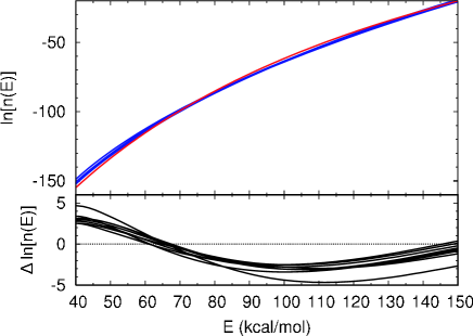
For a WLMD simulation to work at all, good estimate of the density of states should be obtained as the simulation proceeds. We compare the density of states obtained by eight WLMD simulations with that obtained by a long REMD simulation in Fig. 2. Again, we see that the results of the two methods agree quite well. A close examination reveals that WLMD slightly overestimates the density of low energy ( kcal/mol) states (Fig. 2, lower part) compared to REMD. Nevertheless, such difference is of a small fraction () of the entire range of the density of states. Since WLMD is simply a method to efficiently estimate the density of states for multicanonical MD, we can always further refine the density of states using an ordinary multicanonical MD procedure.
We next turn to our main application of WLMD: sampling of low-energy conformations of Trp-cage.

In order to check if the density of states is still accurately estimated for this bigger protein, we plotted the density of states obtained by three independent WLMD simulations (Fig. 3). Although we cannot know the exact density of states, the consistency among these estimates of density of states suggests that the present scheme is at least self-consistent. In order to calculate thermodynamic quantities, one should gradually decrease the value of toward zero and set for the production run, as suggested by Wang and Landau Wang and Landau (2001). In the present example with Trp-cage, our purpose is efficient sampling of low energy conformations but not calculating thermodynamic quantities so that is always kept greater than 0.
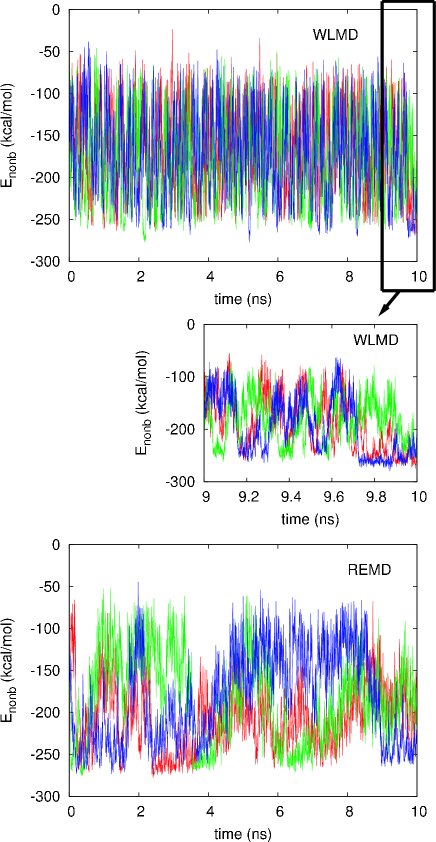
We next compare the (non-bond) energy trajectories of WLMD and REMD simulations (Fig. 4). We selected three trajectories arbitrarily from 24 simulations or replicas. It is immediately apparent that the WLMD trajectories (Fig. 4, upper panel) traverse a wide range of energy very rapidly compared to the REMD trajectories (Fig. 4, lower panel). In fact, one trajectory of REMD seems to be trapped in a local minimum.
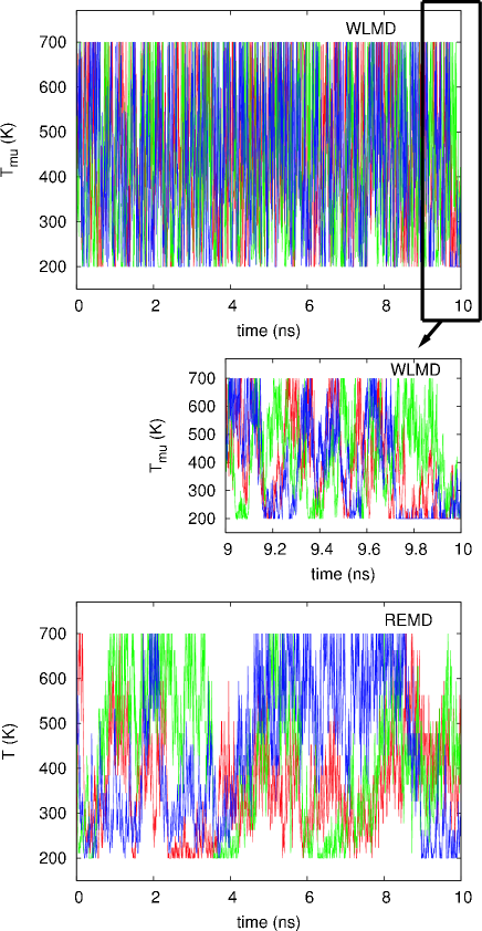
A similar trend is also observed for temperature trajectories (Fig. 5). The multicanonical temperature changes very rapidly but smoothly in WLMD (Fig. 5, upper panel) while the temperature changes rather slowly in REMD (Fig. 5, lower panel). One reason for such a behavior in WLMD is that the multicanonical temperature can vary continuously between (200 K) and (700 K) as it is determined by Eq. (16). On the other hand, in REMD, there are only 24 allowed and fixed temperatures if we use 24 replicas so that the acceptance ratio of temperature swapping can be arbitrarily small.
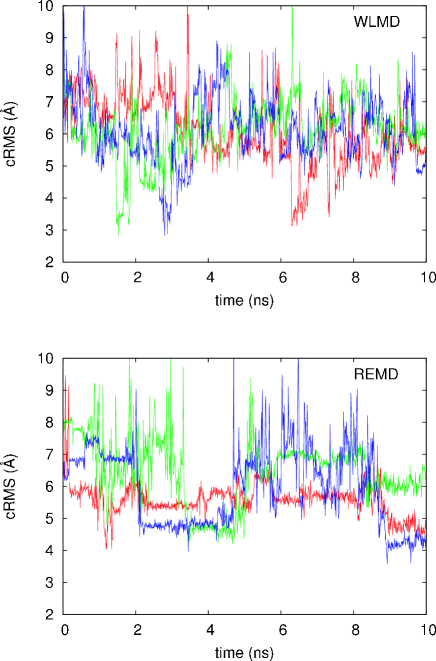
Although rapid traversal of a wide energy or temperature range is necessary, it is not sufficient for efficient sampling of conformational space. In fact, rapid energy change may be associated with very localized motions such as bond stretching. In order to examine the sampling efficiency of WLMD, we first checked the trajectories of the coordinate root mean square deviation (cRMS) from the native structure of Trp-cage (Fig. 6). As expected, cRMS changes more slowly (Fig. 6) than might be suggested by the energy trajectories (Fig. 4) in both WLMD and REMD. Nevertheless, WLMD is much less prone to being trapped in local minima and conformations appear to keep moving compared to REMD. A similar trend was observed for the trajectories of end-to-end distance (not shown).
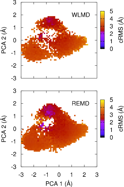
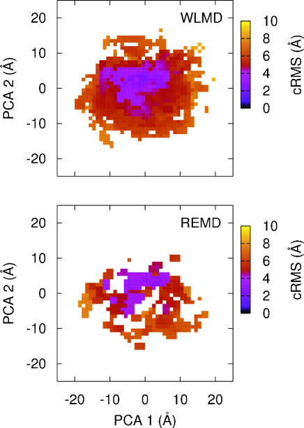
In order to visualize the efficiency of conformational sampling, we carried out principal component analysis Kitao and Go (1999). Out of 1 200 000 conformations saved during 24 WLMD simulations, 50 000 lowest energy conformations were extracted, to which 50 000 lowest energy conformations out of 1 200 000 saved during the REMD simulation (24 replicas) were added. These 100 000 conformations were used to define the principal axes. Conformations sampled in WLMD and REMD were then projected onto the principal space (Fig. 7). It is apparent from Fig. 7 that WLMD covers much more space than REMD. To confirm this observation more quantitatively, we divided the space spanned by the first three principal axes (each from -25 to 25 Å) into small cells (1.0 1.0 1.0 Å3), and counted the number of occupied cells. Out of 125 000 cells, 4 335 (including the cell containing the native structure) were occupied by WLMD while only 1 174 by REMD and the native structure cell was not occupied. Therefore, in terms of the cell occupancy, WLMD is 3.7 times more efficient than REMD for sampling protein conformations.
In summary, we formulated the Wang-Landau molecular dynamics method. In so doing, we adopted the Gaussian masking for updating the density of states, and developed a technique to reliably estimate the multicanonical temperature. It was shown that the WLMD method indeed samples conformational space of a protein more efficiently than the replica exchange MD method. Apart from the inaccuracy in the molecular force field, the present method will serve as a useful tool for simulation studies of protein molecules.
Acknowledgements.
This work was supported in part by a grant-in-aid from the MEXT, Japan.References
- Berg and Neuhaus (1991) B. A. Berg and T. Neuhaus, Phys. Rev. Lett. 68, 9 (1991).
- Hukushima and Nemoto (1996) K. Hukushima and K. Nemoto, J. Phys. Soc. Jpn. 65, 1604 (1996).
- Sugita and Okamoto (1999) Y. Sugita and Y. Okamoto, Chem. Phys. Lett. 314, 141 (1999).
- Wang and Landau (2001) F. Wang and D. P. Landau, Phys. Rev. E 64, 056101 (2001).
- Yamashita et al. (2001) H. Yamashita, S. Endo, H. Wako, and A. Kidera, Chem. Phys. Lett. 342, 382 (2001).
- Åberg et al. (2004) K. M. Åberg, A. P. Lyubartsev, S. P. Jacobsson, and A. Laaksonen, J. Chem. Phys. 120, 3770 (2004).
- Hansmann et al. (1996) U. H. E. Hansmann, Y. Okamoto, and F. Eisenmenger, Chem. Phys. Lett. 259, 321 (1996).
- Nakajima et al. (1997) N. Nakajima, H. Nakamura, and A. Kidera, J. Phys. Chem. B 101, 817 (1997).
- Kumar et al. (1992) S. Kumar, D. Bouzida, R. H. Swendsen, P. A. Kollman, and J. M. Rosenberg, J. Comput. Chem. 13, 1011 (1992).
- Hansmann (1997) U. H. E. Hansmann, Phys. Rev. E 56, 6200 (1997).
- Kim et al. (2003) J. G. Kim, Y. Fukunishi, A. Kidera, and H. Nakamura, Phys. Rev. E 68, 021110 (2003).
- Morikami et al. (1992) K. Morikami, T. Nakai, A. Kidera, M. Saito, and H. Nakamura, Comput. Chem. 16, 243 (1992).
- Kollman et al. (1997) P. Kollman, R. Dixon, W. Cornell, T. Fox, C. Chipot, and A. Pohorille, in Computer Simulation of Biomolecular Systems, edited by A. Wilkinson, P. Weiner, and W. V. Gunsteren (Kluwer/ESCOM, The Netherlands, 1997), Vol. 3, p. 83.
- Neidigh et al. (2002) J. W. Neidigh, R. M. Fesinmeyer, and N. H. Andersen, Nat. Struct. Biol. 9, 408 (2002).
- Simmerling et al. (2002) C. Simmerling, B. Strockbine, and A. E. Roitberg, J. Am. Chem. Soc. 124, 11258 (2002).
- Chowdhury et al. (2003) S. Chowdhury, M. C. Lee, G. Xiong, and Y. Duan, J. Mol. Biol. 327, 711 (2003).
- Zhou (2003) R. Zhou, Proc. Natl. Acad. Sci. USA 100, 13280 (2003).
- Ota et al. (2004) M. Ota, M. Ikeguchi, and A. Kidera, Proc. Natl. Acad. Sci. USA 101, 17658 (2004).
- Ooi et al. (1987) T. Ooi, M. Oobatake, G. Nemethy, and H. A. Scheraga, Proc. Natl. Acad. Sci. USA 84, 3086 (1987).
- (20) A. R. Kinjo, T. Mitsui, T. Nagasima, and K. Nishikawa (unpublished).
- Kitao and Go (1999) A. Kitao and N. Go, Curr. Opin. Struct. Biol. 9, 164 (1999).