Quantum entanglement of decohered two-mode squeezed states in absorbing and amplifying environment

Phoenix S. Y. Poon and C. K. Law Department of Physics and Institute of Theoretical Physics, The Chinese University of Hong Kong, Shatin, Hong Kong SAR, China
Abstract

We investigate the properties of quantum entanglement of two-mode squeezed states interacting with linear baths with general gain and loss parameters. By explicitly solving for ρ𝜌\rho from the master equation, we determine analytical expressions of eigenvalues and eigenvectors of ρTAsuperscript𝜌subscript𝑇𝐴\rho^{T_{A}} (the partial transposition of density matrix ρ𝜌\rho). In Fock space, ρTAsuperscript𝜌subscript𝑇𝐴\rho^{T_{A}} is shown to maintain a block diagonal structure as the system evolves. In addition, we discover that the decoherence induced by the baths would break the degeneracy of ρTAsuperscript𝜌subscript𝑇𝐴\rho^{T_{A}}, and leads to a novel set of eigenvectors for the construction of entanglement witness operators. Such eigenvectors are shown to be time-independent, which is a signature of robust entanglement of two-mode squeezed states in the presence of noise.

pacs:
03.67.Mn, 03.65.Yz, 42.50.Dv, 42.50.Lc

I Introduction

Optical two-mode squeezed vacuum (TMSV) has been a major source of continuous-variable entanglement for quantum communication braunstein . In recent years, intriguing applications such as quantum teleportation teleport1 ; teleport2 ; teleport3 ; teleport4 ; teleport5 and quantum dense coding dense1 ; dense2 have been demonstrated experimentally with TMSV. Theoretically, it is also known that TMSV maximizes the EPR correlation when a fixed amount of entanglement is given cirac2 . In order to exploit fully the non-classical properties of such entangled light fields, it is important to understand decoherence effects as they propagate through noisy environments hiroshima ; positionspace1 ; dodd ; welsch ; Enk ; wigner0 ; ban ; wigner1 ; wigner2 ; char1 . This belongs to a more subtle topic involving the characterization and quantification of mixed state entanglement in general.

For bipartite systems, Peres and Horodecki have developed a powerful criterion of entanglement, which is known as the PPT (positive partial transposition) criterion PPTperes ; PPThoro1 ; PPThoro . If the partial transposition of a density matrix (denoted by ρTAsuperscript𝜌subscript𝑇𝐴\rho^{T_{A}}) has one or more negative eigenvalues, then the state is an entangled state. Physically, the partial transposition for separable states can be considered as a time-reversal operation, and one can construct a variety of uncertainty relations serving as indicators of entanglement Agarwal ; vogel . For two-mode Gaussian states such as TMSV, PPT provides a necessary and sufficient condition of separability Simon ; LMDuan .

The dynamics of disentanglement of TMSV in various noisy situations has been addressed by several authors recently hiroshima ; positionspace1 ; dodd ; welsch ; Enk ; wigner0 ; ban ; wigner1 ; wigner2 ; char1 . The fact that an amplitude damped TMSV remains Gaussian enables an elegant description of entanglement based on the properties of covariance matrix associated with the density operators parisbook . In particular, from the time-dependent solution of Wigner function wigner0 ; ban ; wigner1 or the corresponding characteristic function char1 , one can quantify the degradation of entanglement by calculating the negativity monotone and relative entropy entropy . It is now known that for an initial TMSV at a non-zero thermal bath, quantum entanglement vanishes completely in a finite time parisbook .

However, we notice that there are much less investigations addressing the structure of ρTAsuperscript𝜌subscript𝑇𝐴\rho^{T_{A}} directly, and yet ρTAsuperscript𝜌subscript𝑇𝐴\rho^{T_{A}} is what the PPT criterion originally based upon. Since ρTAsuperscript𝜌subscript𝑇𝐴\rho^{T_{A}} could manifest differently in various basis, the study of ρTAsuperscript𝜌subscript𝑇𝐴\rho^{T_{A}} in Fock space, for example, could reveal entanglement properties not easily found by the Wigner function method detect . An example we notice is the construction of entanglement witness operators via the projectors formed by the eigenvectors of ρTAsuperscript𝜌subscript𝑇𝐴\rho^{T_{A}} with negative eigenvalues entneg . Such entanglement witness operators, which correspond a variety of observables for the detection of entanglement, are determined by ρTAsuperscript𝜌subscript𝑇𝐴\rho^{T_{A}}.

The main purpose of this paper to indicate some key features of decohered entanglement as revealed by eigenvalues and eigenvectors of ρTAsuperscript𝜌subscript𝑇𝐴\rho^{T_{A}}. Our analysis will concentrate on the structures of eigenvectors in Fock space, which is also where interesting non-local correlations of continuous-variable systems can be observed bellpseudospin . For a TMSV under the influence of amplitude damping (or gaining in an amplifier), we solve for the time evolution of ρ𝜌\rho and determine the exact eigenvectors and eigenvalues of ρTAsuperscript𝜌subscript𝑇𝐴\rho^{T_{A}} analytically. These eigenvectors are shown to have a strong correlation in photon numbers, and hence ρTAsuperscript𝜌subscript𝑇𝐴\rho^{T_{A}} is a block diagonal matrix in Fock space. Therefore witness operators associated with each block involve only a finite number of Fock vectors, which implies that the detection of entanglement can only require a small portion of the Hilbert space. This is in contrast to entanglement detection based on uncertainty relations in which the entire Hilbert space is usually involved Agarwal ; vogel ; Simon ; LMDuan . In this sense the eigenvectors of ρTAsuperscript𝜌subscript𝑇𝐴\rho^{T_{A}} access the entanglement signatures β€˜locally’, which is a complement to β€˜global’ characterization (of Gaussian states) using covariance matrices. As we shall see below, as long as the initial state is a TMSV, the corresponding eigenvectors do not change with time, indicating that the entanglement carried by TMSV is robust against amplitude damping.

II Master equation and solution

To begin with, we consider the time evolution of an initial TMSV, each coupled with a separate phase-insensitive linear bath. In terms of the annihilation operators aπ‘Ža and b𝑏b of the two modes, the master equation governing the dynamical process is mandel :

ΟΛ™Λ™πœŒ\displaystyle\dot{\rho} =\displaystyle= G​(2​a†​ρ​aβˆ’a​aβ€ β€‹Οβˆ’Οβ€‹a​a†+2​b†​ρ​bβˆ’b​bβ€ β€‹Οβˆ’Οβ€‹b​b†)𝐺2superscriptπ‘Žβ€ πœŒπ‘Žπ‘Žsuperscriptπ‘Žβ€ πœŒπœŒπ‘Žsuperscriptπ‘Žβ€ 2superscriptπ‘β€ πœŒπ‘π‘superscriptπ‘β€ πœŒπœŒπ‘superscript𝑏†\displaystyle G(2a^{\dagger}\rho a-aa^{\dagger}\rho-\rho aa^{\dagger}+2b^{\dagger}\rho b-bb^{\dagger}\rho-\rho bb^{\dagger})
+\displaystyle+ L​(2​a​ρ​aβ€ βˆ’a†​aβ€‹Οβˆ’Οβ€‹a†​a+2​b​ρ​bβ€ βˆ’b†​bβ€‹Οβˆ’Οβ€‹b†​b),𝐿2π‘ŽπœŒsuperscriptπ‘Žβ€ superscriptπ‘Žβ€ π‘ŽπœŒπœŒsuperscriptπ‘Žβ€ π‘Ž2π‘πœŒsuperscript𝑏†superscriptπ‘β€ π‘πœŒπœŒsuperscript𝑏†𝑏\displaystyle L(2a\rho a^{\dagger}-a^{\dagger}a\rho-\rho a^{\dagger}a+2b\rho b^{\dagger}-b^{\dagger}b\rho-\rho b^{\dagger}b),

where G𝐺G and L𝐿L are the gain and loss parameters respectively, both having a dimension of timeβˆ’1superscripttime1\mbox{time}^{-1}. Depending on the values of G𝐺G and L𝐿L, the master equation describes amplifying or damping effects due to the coupling with the baths. For dissipation in thermal baths, each of temperature T𝑇T, we have the parameters G=Ξ³2​nt​h𝐺𝛾2subscriptπ‘›π‘‘β„ŽG=\frac{\gamma}{2}n_{th} and L=Ξ³2​(nt​h+1)𝐿𝛾2subscriptπ‘›π‘‘β„Ž1L=\frac{\gamma}{2}(n_{th}+1), where nt​h=1exp⁑(h​ω/k​T)βˆ’1subscriptπ‘›π‘‘β„Ž1β„Žπœ”π‘˜π‘‡1n_{th}=\frac{1}{\exp({h\omega/kT})-1} is the average number of photons in each of the modes (with frequency Ο‰πœ”\omega) at thermal equilibrium, and Ξ³/2𝛾2\gamma/2 is the decay rate of the mode amplitudes. In this paper we focus on the initial TMSV with the squeezing parameter r>0π‘Ÿ0r>0:

|Οˆβ€‹(0)⟩=exp⁑[r​(a†​bβ€ βˆ’a​b)]​|00⟩=1βˆ’Ξ»2β€‹βˆ‘n=0∞λn​|n​n⟩,ketπœ“0π‘Ÿsuperscriptπ‘Žβ€ superscriptπ‘β€ π‘Žπ‘ket001superscriptπœ†2subscriptsuperscript𝑛0superscriptπœ†π‘›ket𝑛𝑛\displaystyle\left|\psi(0)\right\rangle=\exp[r(a^{\dagger}b^{\dagger}-ab)]\left|00\right\rangle=\sqrt{1-\lambda^{2}}\sum^{\infty}_{n=0}\lambda^{n}\left|nn\right\rangle, (2)

where λ≑tanh⁑rπœ†π‘Ÿ\lambda\equiv\tanh r and |00⟩ket00\left|00\right\rangle is the two-mode vacuum state.

II.1 Block structures of ρTAsuperscript𝜌subscript𝑇𝐴\rho^{T_{A}} in Fock space

Refer to caption
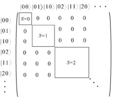
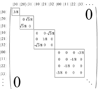
Figure 1: The sub-matrix structure of ρTAsuperscript𝜌subscript𝑇𝐴\rho^{T_{A}}, with initial TMSV, in the Fock basis.

To investigate the entanglement properties of the density matrix ρ𝜌\rho, we study its partial transposition ρTAsuperscript𝜌subscript𝑇𝐴\rho^{T_{A}}. The ρTAsuperscript𝜌subscript𝑇𝐴\rho^{T_{A}} is of infinite dimension, however, by examining the master equation in the Fock basis, block structures of ρTAsuperscript𝜌subscript𝑇𝐴\rho^{T_{A}} can be identified. Let us denote the matrix elements of ρTAsuperscript𝜌subscript𝑇𝐴\rho^{T_{A}} by

ρTAn,m,p,q=⟨n​m|ρTA|p​q⟩=⟨p​m|ρ|n​q⟩,subscriptsuperscript𝜌subscriptπ‘‡π΄π‘›π‘šπ‘π‘žquantum-operator-productπ‘›π‘šsuperscript𝜌subscriptπ‘‡π΄π‘π‘žquantum-operator-productπ‘π‘šπœŒπ‘›π‘ž{\rho^{T_{A}}}_{n,m,p,q}=\left\langle nm|\rho^{T_{A}}|pq\right\rangle=\left\langle pm|\rho|nq\right\rangle, (3)

which is governed by the following differential equation:

ρ˙TAn,m,p,qsubscriptsuperscriptΛ™πœŒsubscriptπ‘‡π΄π‘›π‘šπ‘π‘ž\displaystyle{\dot{\rho}^{T_{A}}}_{n,m,p,q} =\displaystyle= G[2n​pρTAnβˆ’1,m,pβˆ’1,q\displaystyle G[2\sqrt{np}{\rho^{T_{A}}}_{n-1,m,p-1,q} (4)
+2​m​q​ρTAn,mβˆ’1,p,qβˆ’12π‘šπ‘žsubscriptsuperscript𝜌subscriptπ‘‡π΄π‘›π‘š1π‘π‘ž1\displaystyle\ \ +2\sqrt{mq}{\rho^{T_{A}}}_{n,m-1,p,q-1}
βˆ’(n+m+p+q+4)ρTAn,m,p,q]\displaystyle\ \ -(n+m+p+q+4){\rho^{T_{A}}}_{n,m,p,q}]
+L[2(n+1)​(p+1)ρTAn+1,m,p+1,q\displaystyle+L[2\sqrt{(n+1)(p+1)}{\rho^{T_{A}}}_{n+1,m,p+1,q}
+2​(m+1)​(q+1)​ρTAn,m+1,p,q+12π‘š1π‘ž1subscriptsuperscript𝜌subscriptπ‘‡π΄π‘›π‘š1π‘π‘ž1\displaystyle\ \ +2\sqrt{(m+1)(q+1)}{\rho^{T_{A}}}_{n,m+1,p,q+1}
βˆ’(n+m+p+q)ρTAn,m,p,q].\displaystyle\ \ -(n+m+p+q){\rho^{T_{A}}}_{n,m,p,q}].

and

ρTAn,m,p,q​(t=0)=Ξ΄p​m​δn​q​(1βˆ’Ξ»2)​λm+n.subscriptsuperscript𝜌subscriptπ‘‡π΄π‘›π‘šπ‘π‘žπ‘‘0subscriptπ›Ώπ‘π‘šsubscriptπ›Ώπ‘›π‘ž1superscriptπœ†2superscriptπœ†π‘šπ‘›\displaystyle{\rho^{T_{A}}}_{n,m,p,q}(t=0)=\delta_{pm}\delta_{nq}(1-\lambda^{2})\lambda^{m+n}. (5)

corresponds to the initial condition (2).

It can be seen from Eq.Β (4) that each element ρTAn,m,p,q​(t)subscriptsuperscript𝜌subscriptπ‘‡π΄π‘›π‘šπ‘π‘žπ‘‘{\rho^{T_{A}}}_{n,m,p,q}(t) is coupled with elements ρTAn+l,m+k,p+l,q+k​(0)subscriptsuperscript𝜌subscriptπ‘‡π΄π‘›π‘™π‘šπ‘˜π‘π‘™π‘žπ‘˜0{\rho^{T_{A}}}_{n+l,m+k,p+l,q+k}(0) only, for integers l𝑙l and kπ‘˜k. Therefore ρTAn+l,m+k,m+l,n+k​(t)subscriptsuperscript𝜌subscriptπ‘‡π΄π‘›π‘™π‘šπ‘˜π‘šπ‘™π‘›π‘˜π‘‘{\rho^{T_{A}}}_{n+l,m+k,m+l,n+k}\left(t\right) are the only non-zero elements at any time t>0𝑑0t>0 because of the initial condition. By noting that the sum of the first two indices equal to that of the last two, we can group all non-zero elements ρTAn+l,m+k,m+l,n+k​(t)subscriptsuperscript𝜌subscriptπ‘‡π΄π‘›π‘™π‘šπ‘˜π‘šπ‘™π‘›π‘˜π‘‘{\rho^{T_{A}}}_{n+l,m+k,m+l,n+k}\left(t\right) into sub-matrices β„³Ssubscriptℳ𝑆{\cal M}_{S} according to the sum index S=n+l+m+kπ‘†π‘›π‘™π‘šπ‘˜S=n+l+m+k, i.e., ρTAn+l,m+k,m+l,n+k​(t)subscriptsuperscript𝜌subscriptπ‘‡π΄π‘›π‘™π‘šπ‘˜π‘šπ‘™π‘›π‘˜π‘‘{\rho^{T_{A}}}_{n+l,m+k,m+l,n+k}\left(t\right) is contained in β„³n+l+m+ksubscriptβ„³π‘›π‘™π‘šπ‘˜{\cal M}_{n+l+m+k}. We can therefore express ρTAsuperscript𝜌subscript𝑇𝐴\rho^{T_{A}} in a direct sum of β„³Ssubscriptℳ𝑆{\cal M}_{S} as follows:

ρTA​(t)=⨁S=0βˆžβ„³S​(t),superscript𝜌subscript𝑇𝐴𝑑subscriptsuperscriptdirect-sum𝑆0subscriptℳ𝑆𝑑\rho^{T_{A}}(t)=\bigoplus^{\infty}_{S=0}{\cal M}_{S}(t), (6)

where the sub-matrix β„³Ssubscriptℳ𝑆{\cal M}_{S} has a dimension of S+1𝑆1S+1, since elements in β„³Ssubscriptℳ𝑆{\cal M}_{S} have its first two indices as {0,S}0𝑆\{0,S\}, {1,Sβˆ’1}1𝑆1\{1,S-1\}, … , {S,0}𝑆0\{S,0\}. Fig. 1 shows the sub-matrix structure of ρTAsuperscript𝜌subscript𝑇𝐴\rho^{T_{A}}. Note that characteristic sum S𝑆S is equal to the total number of photons that the two modes contain. From Eq.Β (4) we observe that probabilistic flow occurs between elements in neighboring sub-matrices, with emission or absorption of one photon in one of the modes at one time.

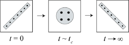
The time evolution of a typical sub-matrix of ρTAsuperscript𝜌subscript𝑇𝐴\rho^{T_{A}} is illustrated schematically in Fig. 2, which will be discussed in detail in the later part of the paper. Initially, only opposite-diagonal elements are present, having the magnitude as Ξ»Ssuperscriptπœ†π‘†\lambda^{S}. As time increases, element flows from neighboring sub-matrices, and disentanglement of the sub-matrices occurs at a critical time t=tc𝑑subscript𝑑𝑐t=t_{c} (Section III.1). In the case of thermal bath, ρTAsuperscript𝜌subscript𝑇𝐴\rho^{T_{A}} evolves into a diagonal form in the long time limit, settling as the thermal equilibrium state ρTAn,m,p,q=Ξ΄n​p​δm​q​1(nt​h+1)2​(nt​hnt​h+1)n+msubscriptsuperscript𝜌subscriptπ‘‡π΄π‘›π‘šπ‘π‘žsubscript𝛿𝑛𝑝subscriptπ›Ώπ‘šπ‘ž1superscriptsubscriptπ‘›π‘‘β„Ž12superscriptsubscriptπ‘›π‘‘β„Žsubscriptπ‘›π‘‘β„Ž1π‘›π‘š{\rho^{T_{A}}}_{n,m,p,q}=\delta_{np}\delta_{mq}\frac{1}{(n_{th}+1)^{2}}(\frac{n_{th}}{n_{th}+1})^{n+m}.

Refer to caption
Figure 2: (Color online) Schematic diagram showing the evolution of the distribution of elements in a sub-matrix of ρTAsuperscript𝜌subscript𝑇𝐴\rho^{T_{A}}, assuming the baths are thermal baths. The tcsubscript𝑑𝑐t_{c} is the critical time for disentanglement.

II.2 Analytic solution of ρ𝜌\rho in position space

To analyze the properties of ρTAsuperscript𝜌subscript𝑇𝐴\rho^{T_{A}}, it is more convenient to first determine ρ𝜌\rho in position space and then make the transformation to Fock space. The position space method of finding ρ𝜌\rho was previously employed in Ref. positionspace1 ; positionspace2 in studying entanglement in various oscillator systems. In this subsection, we present an explicit solution of master equation (1) with an initial TMSV. We remark that our method is different from that given in positionspace1 , as the latter involves a Fourier transform of the density matrix, i.e., the momentum space. Here we solve the density matrix entirely in position space (Appendix A). This turns out to be more convenient for the real symmetric Gaussian states considered here, since fewer differential equations are involved. In addition, the resultant solution is more transparent for further analysis of eigenvectors in the next section.

Let us denote the β€˜position’ operators as x=12​(a+a†)π‘₯12π‘Žsuperscriptπ‘Žβ€ x=\frac{1}{\sqrt{2}}(a+a^{{\dagger}}) and y=12​(b+b†)𝑦12𝑏superscript𝑏†y=\frac{1}{\sqrt{2}}(b+b^{{\dagger}}), and define

ρ​(x1,y1;x2,y2;t)β‰‘βŸ¨x1,y1|ρ​(t)|x2,y2⟩,𝜌subscriptπ‘₯1subscript𝑦1subscriptπ‘₯2subscript𝑦2𝑑quantum-operator-productsubscriptπ‘₯1subscript𝑦1πœŒπ‘‘subscriptπ‘₯2subscript𝑦2\rho(x_{1},y_{1};x_{2},y_{2};t)\equiv\left\langle x_{1},y_{1}\right|\rho(t)\left|x_{2},y_{2}\right\rangle, (7)

then the master equation (1) becomes,

ΟΛ™Λ™πœŒ\displaystyle\dot{\rho} =\displaystyle= βˆ’12[L(x12+x22βˆ’2x1x2+y12+y22βˆ’2y1y2βˆ’4\displaystyle-\frac{1}{2}[L(x_{1}^{2}+x_{2}^{2}-2x_{1}x_{2}+y_{1}^{2}+y_{2}^{2}-2y_{1}y_{2}-4 (8)
βˆ’βˆ‚x12βˆ’βˆ‚x22βˆ’βˆ‚y12βˆ’βˆ‚y22βˆ’2β€‹βˆ‚x1βˆ‚x2βˆ’2β€‹βˆ‚y1βˆ‚y2subscriptsuperscript2subscriptπ‘₯1subscriptsuperscript2subscriptπ‘₯2subscriptsuperscript2subscript𝑦1subscriptsuperscript2subscript𝑦22subscriptsubscriptπ‘₯1subscriptsubscriptπ‘₯22subscriptsubscript𝑦1subscriptsubscript𝑦2\displaystyle-\partial^{2}_{x_{1}}-\partial^{2}_{x_{2}}-\partial^{2}_{y_{1}}-\partial^{2}_{y_{2}}-2\partial_{x_{1}}\partial_{x_{2}}-2\partial_{y_{1}}\partial_{y_{2}}
βˆ’2x1βˆ‚x2βˆ’2x2βˆ‚x1βˆ’2y1βˆ‚y2βˆ’2y2βˆ‚y1)\displaystyle-2x_{1}\partial_{x_{2}}-2x_{2}\partial_{x_{1}}-2y_{1}\partial_{y_{2}}-2y_{2}\partial_{y_{1}})
+G(x12+x22βˆ’2x1x2+y12+y22βˆ’2y1y2+4\displaystyle+G(x_{1}^{2}+x_{2}^{2}-2x_{1}x_{2}+y_{1}^{2}+y_{2}^{2}-2y_{1}y_{2}+4
βˆ’βˆ‚x12βˆ’βˆ‚x22βˆ’βˆ‚y12βˆ’βˆ‚y22βˆ’2β€‹βˆ‚x1βˆ‚x2βˆ’2β€‹βˆ‚y1βˆ‚y2subscriptsuperscript2subscriptπ‘₯1subscriptsuperscript2subscriptπ‘₯2subscriptsuperscript2subscript𝑦1subscriptsuperscript2subscript𝑦22subscriptsubscriptπ‘₯1subscriptsubscriptπ‘₯22subscriptsubscript𝑦1subscriptsubscript𝑦2\displaystyle-\partial^{2}_{x_{1}}-\partial^{2}_{x_{2}}-\partial^{2}_{y_{1}}-\partial^{2}_{y_{2}}-2\partial_{x_{1}}\partial_{x_{2}}-2\partial_{y_{1}}\partial_{y_{2}}
+2x1βˆ‚x2+2x2βˆ‚x1+2y1βˆ‚y2+2y2βˆ‚y1)]ρ.\displaystyle+2x_{1}\partial_{x_{2}}+2x_{2}\partial_{x_{1}}+2y_{1}\partial_{y_{2}}+2y_{2}\partial_{y_{1}})]\rho.

For an initial state (2), ρ​(x1,y1;x2,y2;t)𝜌subscriptπ‘₯1subscript𝑦1subscriptπ‘₯2subscript𝑦2𝑑\rho(x_{1},y_{1};x_{2},y_{2};t) takes a Gaussian form at any time t𝑑t,

ρ​(x1,y1;x2,y2;t)𝜌subscriptπ‘₯1subscript𝑦1subscriptπ‘₯2subscript𝑦2𝑑\displaystyle\rho(x_{1},y_{1};x_{2},y_{2};t) =\displaystyle= Ξ(t)exp[βˆ’A(t)(x12+x22+y12+y22)\displaystyle\Xi(t)\exp[-A(t)(x_{1}^{2}+x_{2}^{2}+y_{1}^{2}+y_{2}^{2}) (9)
+B​(t)​(x1​y1+x2​y2)𝐡𝑑subscriptπ‘₯1subscript𝑦1subscriptπ‘₯2subscript𝑦2\displaystyle+B(t)(x_{1}y_{1}+x_{2}y_{2})
+C​(t)​(x1​x2+y1​y2)𝐢𝑑subscriptπ‘₯1subscriptπ‘₯2subscript𝑦1subscript𝑦2\displaystyle+C(t)(x_{1}x_{2}+y_{1}y_{2})
+D(t)(x1y2+x2y1)],\displaystyle+D(t)(x_{1}y_{2}+x_{2}y_{1})],

where A​(t)𝐴𝑑A(t), B​(t)𝐡𝑑B(t), C​(t)𝐢𝑑C(t) and D​(t)𝐷𝑑D(t) are real time-dependent coefficients, and the normalization factor is:

Ξžβ€‹(t)=1π​[2​A​(t)βˆ’C​(t)]2βˆ’[B​(t)+D​(t)]2.Ξžπ‘‘1πœ‹superscriptdelimited-[]2𝐴𝑑𝐢𝑑2superscriptdelimited-[]𝐡𝑑𝐷𝑑2\displaystyle\Xi(t)=\frac{1}{\pi}\sqrt{[2A(t)-C(t)]^{2}-[B(t)+D(t)]^{2}}. (10)

By substituting Eq.Β (9) into the master equation, the coefficients are found to obey a set of coupled equations that can be solved analytically (Appendix A). For the TMSV considered here, we have,

A​(t)𝐴𝑑\displaystyle A(t) =\displaystyle= 14​[2​A0​η+G+LGβˆ’L​(Ξ·βˆ’1)+⟨x2⟩t2​(⟨x2⟩t2βˆ’βŸ¨x​y⟩t2)],14delimited-[]2subscript𝐴0πœ‚πΊπΏπΊπΏπœ‚1subscriptdelimited-⟨⟩superscriptπ‘₯2𝑑2superscriptsubscriptdelimited-⟨⟩superscriptπ‘₯2𝑑2superscriptsubscriptdelimited-⟨⟩π‘₯𝑦𝑑2\displaystyle\frac{1}{4}[2A_{0}\eta+\frac{G+L}{G-L}(\eta-1)+\frac{\left\langle{x}^{2}\right\rangle_{t}}{2(\left\langle{x}^{2}\right\rangle_{t}^{2}-\left\langle{x}{y}\right\rangle_{t}^{2})}],
B​(t)𝐡𝑑\displaystyle B(t) =\displaystyle= 12​[B0​η+⟨x​y⟩t2​(⟨x2⟩t2βˆ’βŸ¨x​y⟩t2)],12delimited-[]subscript𝐡0πœ‚subscriptdelimited-⟨⟩π‘₯𝑦𝑑2superscriptsubscriptdelimited-⟨⟩superscriptπ‘₯2𝑑2superscriptsubscriptdelimited-⟨⟩π‘₯𝑦𝑑2\displaystyle\frac{1}{2}[B_{0}\eta+\frac{\left\langle{x}{y}\right\rangle_{t}}{2(\left\langle{x}^{2}\right\rangle_{t}^{2}-\left\langle{x}{y}\right\rangle_{t}^{2})}],
C​(t)𝐢𝑑\displaystyle C(t) =\displaystyle= 12​[2​A0​η+G+LGβˆ’L​(Ξ·βˆ’1)βˆ’βŸ¨x2⟩t2​(⟨x2⟩t2βˆ’βŸ¨x​y⟩t2)],12delimited-[]2subscript𝐴0πœ‚πΊπΏπΊπΏπœ‚1subscriptdelimited-⟨⟩superscriptπ‘₯2𝑑2superscriptsubscriptdelimited-⟨⟩superscriptπ‘₯2𝑑2superscriptsubscriptdelimited-⟨⟩π‘₯𝑦𝑑2\displaystyle\frac{1}{2}[2A_{0}\eta+\frac{G+L}{G-L}(\eta-1)-\frac{\left\langle{x}^{2}\right\rangle_{t}}{2(\left\langle{x}^{2}\right\rangle_{t}^{2}-\left\langle{x}{y}\right\rangle_{t}^{2})}],
D​(t)𝐷𝑑\displaystyle D(t) =\displaystyle= 12​[βˆ’B0​η+⟨x​y⟩t2​(⟨x2⟩t2βˆ’βŸ¨x​y⟩t2)].12delimited-[]subscript𝐡0πœ‚subscriptdelimited-⟨⟩π‘₯𝑦𝑑2superscriptsubscriptdelimited-⟨⟩superscriptπ‘₯2𝑑2superscriptsubscriptdelimited-⟨⟩π‘₯𝑦𝑑2\displaystyle\frac{1}{2}[-B_{0}\eta+\frac{\left\langle{x}{y}\right\rangle_{t}}{2(\left\langle{x}^{2}\right\rangle_{t}^{2}-\left\langle{x}{y}\right\rangle_{t}^{2})}]. (11)

Here A0=12​cosh⁑2​rsubscript𝐴0122π‘ŸA_{0}=\frac{1}{2}\cosh 2r, B0=sinh⁑2​rsubscript𝐡02π‘ŸB_{0}=\sinh 2r and η​(t)=exp⁑[2​(Gβˆ’L)​t]πœ‚π‘‘2𝐺𝐿𝑑\eta(t)=\exp[2(G-L)t] are defined, and the expectation values are given by,

⟨x2⟩tsubscriptdelimited-⟨⟩superscriptπ‘₯2𝑑\displaystyle\left\langle{x}^{2}\right\rangle_{t} =\displaystyle= A0​η+G+L2​(Gβˆ’L)​(Ξ·βˆ’1),subscript𝐴0πœ‚πΊπΏ2πΊπΏπœ‚1\displaystyle A_{0}\eta+\frac{G+L}{2(G-L)}(\eta-1),
⟨x​y⟩tsubscriptdelimited-⟨⟩π‘₯𝑦𝑑\displaystyle\left\langle{x}{y}\right\rangle_{t} =\displaystyle= B02​η.subscript𝐡02πœ‚\displaystyle\frac{B_{0}}{2}\eta. (12)

III Properties of ρTAsuperscript𝜌subscript𝑇𝐴\rho^{T_{A}}

According to PPT criterion, the appearance of negative eigenvalues of ρTAsuperscript𝜌subscript𝑇𝐴\rho^{T_{A}} is a signature of entanglement. In this section, we solve the eigenvectors and eigenvalues of ρTAsuperscript𝜌subscript𝑇𝐴\rho^{T_{A}} as the system evolves. Then we discuss how decoherence affects the entanglement properties of ρTAsuperscript𝜌subscript𝑇𝐴\rho^{T_{A}}. The eigenvalues and eigenvectors of ρTAsuperscript𝜌subscript𝑇𝐴\rho^{T_{A}} are defined by:

∫∫ρTA​(x1,y1;x2,y2;t)​φn,m​(x2,y2;t)​𝑑x2​𝑑y2superscript𝜌subscript𝑇𝐴subscriptπ‘₯1subscript𝑦1subscriptπ‘₯2subscript𝑦2𝑑subscriptπœ‘π‘›π‘šsubscriptπ‘₯2subscript𝑦2𝑑differential-dsubscriptπ‘₯2differential-dsubscript𝑦2\displaystyle\int\int\rho^{T_{A}}(x_{1},y_{1};x_{2},y_{2};t)\varphi_{n,m}(x_{2},y_{2};t)dx_{2}dy_{2}
=ΞΎn,m​(t)​φn,m​(x1,y1;t).absentsubscriptπœ‰π‘›π‘šπ‘‘subscriptπœ‘π‘›π‘šsubscriptπ‘₯1subscript𝑦1𝑑\displaystyle=\xi_{n,m}(t)\varphi_{n,m}(x_{1},y_{1};t). (13)

Our main technique of solving the eigen-problem is the use of Mehler formula which expands a double Gaussian function into a series of orthogonal functions. After some calculations (see Appendix B), we obtain the expression of eigenvalues,

ΞΎn,m​(t)=Ξžβ€‹(t)​π​(Ξ±1βˆ’Ξ²1)n(Ξ±1+Ξ²1)n+1​(Ξ±2βˆ’Ξ²2)m(Ξ±2+Ξ²2)m+1subscriptπœ‰π‘›π‘šπ‘‘Ξžπ‘‘πœ‹superscriptsubscript𝛼1subscript𝛽1𝑛superscriptsubscript𝛼1subscript𝛽1𝑛1superscriptsubscript𝛼2subscript𝛽2π‘šsuperscriptsubscript𝛼2subscript𝛽2π‘š1\displaystyle\xi_{n,m}(t)=\Xi(t)\pi\frac{(\sqrt{\alpha_{1}}-\sqrt{\beta_{1}})^{n}}{(\sqrt{\alpha_{1}}+\sqrt{\beta_{1}})^{n+1}}\frac{(\sqrt{\alpha_{2}}-\sqrt{\beta_{2}})^{m}}{(\sqrt{\alpha_{2}}+\sqrt{\beta_{2}})^{m+1}} (14)

and the corresponding eigenvectors,

Ο†n,m​(x1,y1)subscriptπœ‘π‘›π‘šsubscriptπ‘₯1subscript𝑦1\displaystyle\varphi_{n,m}(x_{1},y_{1}) =\displaystyle= 12n+m​n!​m!​π​Hn​(x1βˆ’y12)​Hm​(x1+y12)1superscript2π‘›π‘šπ‘›π‘šπœ‹subscript𝐻𝑛subscriptπ‘₯1subscript𝑦12subscriptπ»π‘šsubscriptπ‘₯1subscript𝑦12\displaystyle\frac{1}{\sqrt{2^{n+m}n!m!\pi}}H_{n}(\frac{x_{1}-y_{1}}{\sqrt{2}})H_{m}(\frac{x_{1}+y_{1}}{\sqrt{2}}) (15)
Γ—exp⁑[βˆ’12​(x12+y12)]absent12superscriptsubscriptπ‘₯12superscriptsubscript𝑦12\displaystyle\times\exp[-\frac{1}{2}(x_{1}^{2}+y_{1}^{2})]

where Hnsubscript𝐻𝑛H_{n} are the Hermite polynomials. In writing Eq.Β (14), we have defined

Ξ±1​(t)=14​[2​A​(t)βˆ’B​(t)+C​(t)+D​(t)],subscript𝛼1𝑑14delimited-[]2𝐴𝑑𝐡𝑑𝐢𝑑𝐷𝑑\displaystyle\alpha_{1}(t)=\frac{1}{4}[2A(t)-B(t)+C(t)+D(t)],
Ξ²1​(t)=14​[2​A​(t)+B​(t)βˆ’C​(t)+D​(t)],subscript𝛽1𝑑14delimited-[]2𝐴𝑑𝐡𝑑𝐢𝑑𝐷𝑑\displaystyle\beta_{1}(t)=\frac{1}{4}[2A(t)+B(t)-C(t)+D(t)],
Ξ±2​(t)=14​[2​A​(t)+B​(t)+C​(t)βˆ’D​(t)],subscript𝛼2𝑑14delimited-[]2𝐴𝑑𝐡𝑑𝐢𝑑𝐷𝑑\displaystyle\alpha_{2}(t)=\frac{1}{4}[2A(t)+B(t)+C(t)-D(t)],
Ξ²2​(t)=14​[2​A​(t)βˆ’B​(t)βˆ’C​(t)βˆ’D​(t)]subscript𝛽2𝑑14delimited-[]2𝐴𝑑𝐡𝑑𝐢𝑑𝐷𝑑\displaystyle\beta_{2}(t)=\frac{1}{4}[2A(t)-B(t)-C(t)-D(t)] (16)

and the solution of A𝐴A, B𝐡B, C𝐢C and D𝐷D are given by Eq.Β (II.2). Note that in writing Eq.Β (15) from (B8), we have used the fact that for TMSV, Ξ±1​β1=Ξ±2​β2=116subscript𝛼1subscript𝛽1subscript𝛼2subscript𝛽2116\alpha_{1}\beta_{1}=\alpha_{2}\beta_{2}=\frac{1}{16} for all time tβ‰₯0𝑑0t\geq 0.

We now transform the eigenvectors from the position space to the Fock space. Note that ρTAsuperscript𝜌subscript𝑇𝐴\rho^{T_{A}} is a basis dependent operation. The eigenvectors of ρTAsuperscript𝜌subscript𝑇𝐴\rho^{T_{A}} defined in two different basis sets do not transform directly. An exception is the case when the two sets of basis vectors transform by a real unitary matrix PTbasisdep , which is the case here. This allows us to write down the eigenvector |Ο†n,m⟩ketsubscriptπœ‘π‘›π‘š\left|\varphi_{n,m}\right\rangle in Fock space from Eq.Β (15):

|Ο†n,m⟩=[1n!​(aβ€ βˆ’b†2)n]​[1m!​(a†+b†2)m]​|00⟩,ketsubscriptπœ‘π‘›π‘šdelimited-[]1𝑛superscriptsuperscriptπ‘Žβ€ superscript𝑏†2𝑛delimited-[]1π‘šsuperscriptsuperscriptπ‘Žβ€ superscript𝑏†2π‘šket00\left|\varphi_{n,m}\right\rangle=[\frac{1}{\sqrt{n!}}(\frac{a^{\dagger}-b^{\dagger}}{\sqrt{2}})^{n}][\frac{1}{\sqrt{m!}}(\frac{a^{\dagger}+b^{\dagger}}{\sqrt{2}})^{m}]\left|00\right\rangle, (17)

which can be connected to the sub-matrices of ρTAsuperscript𝜌subscript𝑇𝐴\rho^{T_{A}} (Fig. 1) via the photon number sum S≑m+nπ‘†π‘šπ‘›S\equiv m+n to label the eigenket, so that

|Ο†n,Sβˆ’n⟩ketsubscriptπœ‘π‘›π‘†π‘›\displaystyle\left|\varphi_{n,S-n}\right\rangle =\displaystyle= 12S​n!​(Sβˆ’n)!1superscript2𝑆𝑛𝑆𝑛\displaystyle\frac{1}{\sqrt{2^{S}}\sqrt{n!(S-n)!}} (18)
Γ—βˆ‘j=0SΞ“S,n,jj!​(Sβˆ’j)!|j,Sβˆ’j⟩.\displaystyle\times\sum^{S}_{j=0}\Gamma_{S,n,j}\sqrt{j!(S-j)!}\left|j,S-j\right\rangle.

Here we have used the abbreviation

Ξ“S,n,jβ‰‘βˆ‘k=0min⁑(j,n)(βˆ’1)nβˆ’k​Cjβˆ’kSβˆ’n​Ckn,subscriptΓ𝑆𝑛𝑗subscriptsuperscriptπ‘—π‘›π‘˜0superscript1π‘›π‘˜subscriptsuperscriptπΆπ‘†π‘›π‘—π‘˜subscriptsuperscriptπΆπ‘›π‘˜\Gamma_{S,n,j}\equiv\sum^{\min(j,n)}_{k=0}(-1)^{n-k}C^{S-n}_{j-k}C^{n}_{k}, (19)

with CrS≑S!r!​(Sβˆ’r)!subscriptsuperscriptπΆπ‘†π‘Ÿπ‘†π‘Ÿπ‘†π‘ŸC^{S}_{r}\equiv\frac{S!}{r!(S-r)!}. In this way |Ο†n,Sβˆ’n⟩ketsubscriptπœ‘π‘›π‘†π‘›\left|\varphi_{n,S-n}\right\rangle and ΞΎn,Sβˆ’nsubscriptπœ‰π‘›π‘†π‘›\xi_{n,S-n} (n=0,1,…,S)𝑛01…𝑆(n=0,1,...,S) are the nt​hsuperscriptπ‘›π‘‘β„Žn^{th} eigenvector and eigenvalue of the block with characteristic sum S𝑆S.

III.1 Evolution of negative eigenvalues
Refer to caption
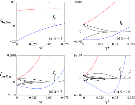
Figure 3: (Color online) The eigenvalues of sub-matrices of ρTAsuperscript𝜌subscript𝑇𝐴\rho^{T_{A}} of an amplifier system with G=1.5​γ𝐺1.5𝛾G=1.5\gamma, L=0.5​γ𝐿0.5𝛾L=0.5\gamma and initial squeezing factor r=tanhβˆ’1⁑0.2π‘Ÿsuperscript10.2r=\tanh^{-1}0.2, with characteristic sum (a) S=1𝑆1S=1, (b) S=4𝑆4S=4, (c) S=7𝑆7S=7, and (d) S=10𝑆10S=10. Red line indicates the n=0𝑛0n=0 eigenvalue which does not turn zero at tcsubscript𝑑𝑐t_{c}, while blue line indicates the most negative eigenvalue with n=1𝑛1n=1.

By inspecting Eq.Β (14), we find that all the negative eigenvalues in each block share the same value at t=0𝑑0t=0 (Fig. 3). The same is true also for positive eigenvalues. However, such a strong degeneracy is broken by coupling with the baths. This is illustrated in Fig. 3 where the time-dependence of individual eigenvalues in various block indices S𝑆S is shown. Except at t=0𝑑0t=0 and at the critical time tcsubscript𝑑𝑐t_{c}, we see that the negative eigenvalues possessing different values.

It is important to observe that the eigenvalues are negative for odd n𝑛n, when Ξ±1<Ξ²1subscript𝛼1subscript𝛽1\sqrt{\alpha_{1}}<\sqrt{\beta_{1}}, or in other words, B​(t)>C​(t)𝐡𝑑𝐢𝑑B(t)>C(t). All eigenvalues turn zero at the same time, when we have B​(t)=C​(t)𝐡𝑑𝐢𝑑B(t)=C(t), except for the only eigenvalue with n=0𝑛0n=0 in each block. Such a critical time tcsubscript𝑑𝑐t_{c} is given by,

tc=12​(Lβˆ’G)​log⁑(G+L​λG​(1+Ξ»))subscript𝑑𝑐12πΏπΊπΊπΏπœ†πΊ1πœ†t_{c}=\frac{{1}}{{2\left({L-G}\right)}}\log\left({\frac{{G+L\lambda}}{{G\left({1+\lambda}\right)}}}\right) (20)

which is always positive finite as long as Gβ‰ 0𝐺0G\not=0. For the case Gβ†’0→𝐺0G\rightarrow 0, we have tcβ†’βˆžβ†’subscript𝑑𝑐t_{c}\rightarrow\infty. We remark that the disentanglement time tcsubscript𝑑𝑐t_{c} was previous obtained in Ref. LMDuan for thermal baths, here we obtained a general expression (20) that applies to linear amplifiers as well. In particular, in the case when gain and loss parameters are equal, i.e., G=L𝐺𝐿G=L, the critical time can be reduced to tc=12​G​λ1+Ξ»>0subscript𝑑𝑐12πΊπœ†1πœ†0t_{c}=\frac{1}{2G}\frac{\lambda}{1+\lambda}>0.

We point out that at the time of disentanglement t=tc𝑑subscript𝑑𝑐t=t_{c}, there is only one non-zero eigenvalue (with the index n=0𝑛0n=0) in each sub-matrix (Fig. 3). Therefore ρTAsuperscript𝜌subscript𝑇𝐴\rho^{T_{A}} at the critical time is highly degenerate, and the corresponding symmetry property of ρTA​(t=tc)superscript𝜌subscript𝑇𝐴𝑑subscript𝑑𝑐\rho^{T_{A}}(t=t_{c}) is indicated in the relation:

ρTAj,Sβˆ’j,j,Sβˆ’j=ρTAj,Sβˆ’j,Sβˆ’j,jsubscriptsuperscript𝜌subscript𝑇𝐴𝑗𝑆𝑗𝑗𝑆𝑗subscriptsuperscript𝜌subscript𝑇𝐴𝑗𝑆𝑗𝑆𝑗𝑗\displaystyle{\rho^{T_{A}}}_{j,S-j,j,S-j}={\rho^{T_{A}}}_{j,S-j,S-j,j}
=ρTASβˆ’j,j,j,Sβˆ’j=ρTASβˆ’j,j,Sβˆ’j,j.absentsubscriptsuperscript𝜌subscript𝑇𝐴𝑆𝑗𝑗𝑗𝑆𝑗subscriptsuperscript𝜌subscript𝑇𝐴𝑆𝑗𝑗𝑆𝑗𝑗\displaystyle={\rho^{T_{A}}}_{S-j,j,j,S-j}={\rho^{T_{A}}}_{S-j,j,S-j,j}. (21)

This results in the symmetric distribution of elements as shown in Fig. 2 schematically.

As a further remark, it is interesting that negative eigenvalues may not necessarily be monotones over time. This can be seen by differentiating Eq.Β (14) and looking at the initial rate:

ΞΎΛ™n,Sβˆ’n|t=0evaluated-atsubscriptΛ™πœ‰π‘›π‘†π‘›π‘‘0\displaystyle\left.\dot{\xi}_{n,S-n}\right|_{t=0} =\displaystyle= (βˆ’1)n​tanhS⁑r​cschr​sech3rsuperscript1𝑛superscriptπ‘†π‘Ÿcschπ‘Ÿsuperscriptsech3π‘Ÿ\displaystyle(-1)^{n}\tanh^{S}r\mathop{\mathrm{csch}}r{\mathop{\mathrm{sech}}}^{3}r (22)
Γ—{(Gβˆ’L)(Sβˆ’2n)\displaystyle\times\{(G-L)(S-2n)
+(G+L)​(Sβˆ’2​n)​cosh⁑2​r𝐺𝐿𝑆2𝑛2π‘Ÿ\displaystyle\ \ +(G+L)(S-2n)\cosh 2r
βˆ’[LS+G(2+S)]sinh2r},\displaystyle\ \ -[LS+G(2+S)]\sinh 2r\},

which can result in a negative value for certain parameters, i.e., some eigenvalues of odd n𝑛n can become more negative over time (Fig. 3d). An exceptional case is when G=0𝐺0G=0, where we find that for odd n𝑛n, the derivative at t=0𝑑0t=0 must be positive by inspecting Eq.Β (22).

Refer to caption
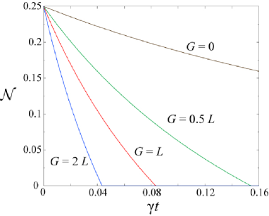
Figure 4: (Color online) The negativity 𝒩𝒩{\cal N} of ρTAsuperscript𝜌subscript𝑇𝐴\rho^{T_{A}} with different G𝐺G, fixing the parameters L=γ𝐿𝛾L=\gamma and initial squeezing factor r=tanhβˆ’1⁑0.2π‘Ÿsuperscript10.2r=\tanh^{-1}0.2.

III.2 Negativity and sub-negativity

Negativity 𝒩𝒩{\cal N} serves as a computable measure of entanglement defined by the trace norm of ρTAsuperscript𝜌subscript𝑇𝐴\rho^{T_{A}} minus 1 divided by 2 monotone . For separable states, ρTAsuperscript𝜌subscript𝑇𝐴\rho^{T_{A}} is still a density matrix with trace 1 and hence 𝒩=0𝒩0{\cal N}=0. However, for non-separable states with negative ρTAsuperscript𝜌subscript𝑇𝐴\rho^{T_{A}}, we have 𝒩>0𝒩0{\cal N}>0. Specifically, 𝒩𝒩{\cal N} equals the sum of the absolute value of negative eigenvalues of ρTAsuperscript𝜌subscript𝑇𝐴\rho^{T_{A}} monotone ; negeigenadd . For the system considered in this paper, 𝒩𝒩{\cal N} reads,

𝒩=Ο€β€‹Ξžβ€‹(t)8​(1Ξ±1​β2βˆ’1Ξ²1​β2).π’©πœ‹Ξžπ‘‘81subscript𝛼1subscript𝛽21subscript𝛽1subscript𝛽2\displaystyle{\cal N}=\frac{\pi\Xi(t)}{8}(\frac{1}{\sqrt{\alpha_{1}\beta_{2}}}-\frac{1}{\sqrt{\beta_{1}\beta_{2}}}). (23)

Alternatively, 𝒩𝒩{\cal N} can be derived from the symplectic spectrum of the covariance matrix associated with the density operator parisbook . In Fig. 4 we show the time evolution of negativity 𝒩𝒩{\cal N} for initial TMSV with different G𝐺G parameters. An example for the G=0𝐺0G=0 case is the zero-temperature bath dissipation scenario. Fixing L𝐿L, we observe that a larger gain G𝐺G leads to a shorter tcsubscript𝑑𝑐t_{c}.

We can also calculate the negativity in a sub-matrix β„³Ssubscriptℳ𝑆{\cal M}_{S}, which measures the contribution of entanglement from the corresponding block that builds up ρTAsuperscript𝜌subscript𝑇𝐴\rho^{T_{A}}. Specifically, the sub-matrix negativity 𝒩Ssubscript𝒩𝑆{\cal N}_{S} is defined the same way as negativity 𝒩𝒩{\cal N} but restricted to the sub-matrix of ρTAsuperscript𝜌subscript𝑇𝐴\rho^{T_{A}} with the characteristic sum S𝑆S. To our knowledge, such a sub-matrix negativity, which requires the calculations of individual eigenvalues, has not been discussed before. Explicitly, 𝒩Ssubscript𝒩𝑆{\cal N}_{S} takes the form:

𝒩S=βˆ’Ο€β€‹Ξžβ€‹(t)β€‹βˆ‘n=0P(Ξ±1βˆ’Ξ²1)2​n+1(Ξ±1+Ξ²1)2​n+2​(Ξ±2βˆ’Ξ²2)Sβˆ’2​nβˆ’1(Ξ±2+Ξ²2)Sβˆ’2​nsubscriptπ’©π‘†πœ‹Ξžπ‘‘subscriptsuperscript𝑃𝑛0superscriptsubscript𝛼1subscript𝛽12𝑛1superscriptsubscript𝛼1subscript𝛽12𝑛2superscriptsubscript𝛼2subscript𝛽2𝑆2𝑛1superscriptsubscript𝛼2subscript𝛽2𝑆2𝑛{\cal N}_{S}=-\pi\Xi(t)\sum^{P}_{n=0}\frac{(\sqrt{\alpha_{1}}-\sqrt{\beta_{1}})^{2n+1}}{(\sqrt{\alpha_{1}}+\sqrt{\beta_{1}})^{2n+2}}\frac{(\sqrt{\alpha_{2}}-\sqrt{\beta_{2}})^{S-2n-1}}{(\sqrt{\alpha_{2}}+\sqrt{\beta_{2}})^{S-2n}} (24)

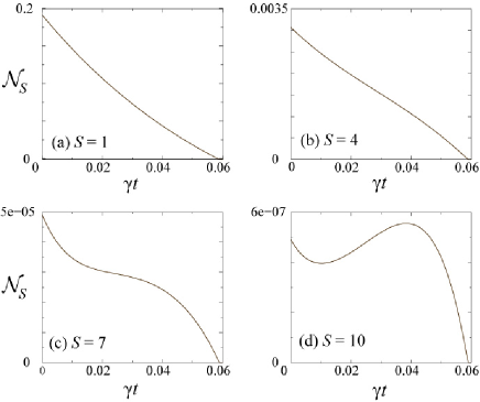
where P𝑃P is defined as the integral part of Sβˆ’12𝑆12\frac{S-1}{2}. In Fig. 5 the behavior of 𝒩Ssubscript𝒩𝑆{\cal N}_{S} of some blocks is illustrated. It is surprising that that for higher sub-matrices the corresponding negativity 𝒩Ssubscript𝒩𝑆{\cal N}_{S} may increase over time. Physically, the increase of 𝒩Ssubscript𝒩𝑆{\cal N}_{S} is due to the probability flow in Fock space arising from damping or amplifying mechanisms. Since each sub-matrix of ρTAsuperscript𝜌subscript𝑇𝐴\rho^{T_{A}} does not necessarily conserve probability (i.e., the trace of β„³Ssubscriptℳ𝑆{\cal M}_{S} is not a constant), it is possible that some blocks could have their negativity increasing with time.

However, the increase of 𝒩Ssubscript𝒩𝑆{\cal N}_{S} does not violate the fact that the overall negativity 𝒩𝒩{\cal N} of ρTAsuperscript𝜌subscript𝑇𝐴\rho^{T_{A}} is an entanglement monotone that does not increase under LOCC (the master equation corresponds to local operations). Eq.Β (14) reveals that eigenvalues of higher blocks are of smaller order of magnitude. As we see in Fig. 5, although negativity of individual higher sub-matrices may increase over time, their contribution for negativity is smaller by several orders than the sub-matrices with lower S𝑆S, and therefore the overall negativity is still monotonic decreasing.
Refer to caption
Figure 5: The negativity of sub-matrices 𝒩Ssubscript𝒩𝑆{\cal N}_{S} of ρTAsuperscript𝜌subscript𝑇𝐴\rho^{T_{A}}, for an amplifier system with G=1.5​γ𝐺1.5𝛾G=1.5\gamma, L=0.5​γ𝐿0.5𝛾L=0.5\gamma and initial squeezing factor r=tanhβˆ’1⁑0.2π‘Ÿsuperscript10.2r=\tanh^{-1}0.2, with characteristic sum (a) S=1𝑆1S=1, (b) S=4𝑆4S=4, (c) S=7𝑆7S=7, and (d) S=10𝑆10S=10.

III.3 Robust structure of entanglement witness

An entanglement witness operator 𝒲𝒲{\cal W} is designed for the detection of entanglement such that T​r​(ρ​𝒲)<0π‘‡π‘ŸπœŒπ’²0Tr(\rho{\cal W})<0 for some non-separable states ρ𝜌\rho, but T​r​(ρs​e​p​𝒲)β‰₯0π‘‡π‘ŸsubscriptπœŒπ‘ π‘’π‘π’²0Tr(\rho_{sep}{\cal W})\geq 0 for all separable states ρs​e​psubscriptπœŒπ‘ π‘’π‘\rho_{sep} PPThoro1 . For each eigenvector |Ο•βŸ©ketitalic-Ο•|\phi\rangle of ρTAsuperscript𝜌subscript𝑇𝐴\rho^{T_{A}} with a negative eigenvalue, one can construct an 𝒲𝒲{\cal W} by 𝒲=|Ο•βŸ©β€‹βŸ¨Ο•|TA𝒲ketitalic-Ο•superscriptbraitalic-Ο•subscript𝑇𝐴{\cal W}=|\phi\rangle\langle\phi|^{T_{A}} entneg meeting the criteria above. In our system, we can construct a family of 𝒲𝒲{\cal W} from eigenvectors |Ο†n,Sβˆ’n⟩ketsubscriptπœ‘π‘›π‘†π‘›\left|\varphi_{n,S-n}\right\rangle with odd n𝑛n accordingly, i.e., 𝒲S,n=|Ο†n,Sβˆ’nβŸ©β€‹βŸ¨Ο†n,Sβˆ’n|TAsubscript𝒲𝑆𝑛ketsubscriptπœ‘π‘›π‘†π‘›superscriptbrasubscriptπœ‘π‘›π‘†π‘›subscript𝑇𝐴{\cal W}_{S,n}=\left|\varphi_{n,S-n}\right\rangle\left\langle\varphi_{n,S-n}\right|^{T_{A}}. From Eq.Β (18), the explicit form of 𝒲S,nsubscript𝒲𝑆𝑛{\cal W}_{S,n} reads,

𝒲S,nsubscript𝒲𝑆𝑛\displaystyle{\cal W}_{S,n} =\displaystyle= βˆ‘j=0Sβˆ‘l=0S{12S​n!​(Sβˆ’n)!Ξ“S,n,jΞ“S,n,l\displaystyle\sum^{S}_{j=0}\sum^{S}_{l=0}\{\frac{1}{{2}^{S}{n!(S-n)!}}\Gamma_{S,n,j}\Gamma_{S,n,l}
Γ—j!​(Sβˆ’j)!​l!​(Sβˆ’l)!}|l,Sβˆ’j⟩⟨j,Sβˆ’l|,\displaystyle\times\sqrt{j!(S-j)!l!(S-l)!}\}\left|l,S-j\right\rangle\left\langle j,S-l\right|,

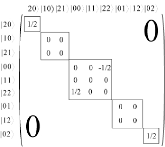
which shows that 𝒲S,nsubscript𝒲𝑆𝑛{\cal W}_{S,n} operates in only a finite dimension in the Fock space. Note that T​r​(ρ​𝒲S,n)=ΞΎn,Sβˆ’nπ‘‡π‘ŸπœŒsubscript𝒲𝑆𝑛subscriptπœ‰π‘›π‘†π‘›Tr(\rho{\cal W}_{S,n})=\xi_{n,S-n}, and ΞΎ1,Sβˆ’1subscriptπœ‰1𝑆1\xi_{1,S-1} is the most negative eigenvalue in each sub-matrix, therefore 𝒲S,1subscript𝒲𝑆1{\cal W}_{S,1} provides the most significant entanglement detection among all witnesses constructed from vectors lying within the sub-matrix β„³Ssubscriptℳ𝑆{\cal M}_{S}. Some examples for entanglement witnesses with n=1𝑛1n=1 are shown in Fig. 6 and Fig. 7.

We observe that 𝒲𝒲{\cal W} also has a block diagonal structure in which non-zero elements are: ⟨j,Sβˆ’l|𝒲S,n|l,Sβˆ’j⟩quantum-operator-product𝑗𝑆𝑙subscript𝒲𝑆𝑛𝑙𝑆𝑗\left\langle j,S-l\right|{\cal W}_{S,n}\left|l,S-j\right\rangle. This allows us to divide 𝒲𝒲{\cal W} into sub-blocks Ξ›KsubscriptΛ𝐾\Lambda_{K}, with each sub-block characterized by a difference K∈[βˆ’S,S]𝐾𝑆𝑆K\in[-S,S]:

𝒲S,n=⨁K=βˆ’SSΞ›K,subscript𝒲𝑆𝑛subscriptsuperscriptdirect-sum𝑆𝐾𝑆subscriptΛ𝐾{\cal W}_{S,n}=\bigoplus^{S}_{K=-S}\Lambda_{K}, (26)

where the element ⟨j,Sβˆ’l|𝒲S,n|l,Sβˆ’j⟩quantum-operator-product𝑗𝑆𝑙subscript𝒲𝑆𝑛𝑙𝑆𝑗\left\langle j,S-l\right|{\cal W}_{S,n}\left|l,S-j\right\rangle lies in the sub-block with K=Sβˆ’jβˆ’l𝐾𝑆𝑗𝑙K=S-j-l. The explicit form of Ξ›KsubscriptΛ𝐾\Lambda_{K} is

Ξ›KsubscriptΛ𝐾\displaystyle\Lambda_{K} =\displaystyle= βˆ‘l=max⁑(0,βˆ’K)min⁑(S,Sβˆ’K){12S​n!​(Sβˆ’n)!Ξ“S,n,Sβˆ’Kβˆ’lΞ“S,n,l\displaystyle\sum^{\min(S,S-K)}_{l=\max(0,-K)}\{\frac{1}{{2}^{S}{n!(S-n)!}}\Gamma_{S,n,S-K-l}\Gamma_{S,n,l} (27)
Γ—(Sβˆ’Kβˆ’l)!​(K+l)!​l!​(Sβˆ’l)!}\displaystyle\times\sqrt{(S-K-l)!(K+l)!l!(S-l)!}\}
|l,K+lβŸ©β€‹βŸ¨Sβˆ’Kβˆ’l,Sβˆ’l|,ket𝑙𝐾𝑙bra𝑆𝐾𝑙𝑆𝑙\displaystyle\ \ \ \left|l,K+l\right\rangle\left\langle S-K-l,S-l\right|,

having a dimension of Sβˆ’|K|+1𝑆𝐾1S-|K|+1. We remark that the simplest 2Γ—2222\times 2 entanglement witness 𝒲1,1subscript𝒲11{\cal W}_{1,1} was constructed in witnessexplicit using a different approach. Here our general 𝒲S,nsubscript𝒲𝑆𝑛{\cal W}_{S,n} applies to all S𝑆S and n𝑛n.

Refer to caption
Figure 6: Example of entanglement witness 𝒲2,1subscript𝒲21{\cal W}_{2,1}.
Refer to caption
Figure 7: Part of the entanglement witness 𝒲3,1subscript𝒲31{\cal W}_{3,1}, showing the blocks with characteristic difference from -3 to 0. 𝒲3,1subscript𝒲31{\cal W}_{3,1} is symmetric about the top-right to bottom-left diagonal.

Finally, let us emphasize the robustness feature of TMSV against decoherence. We have seen from Eq.Β (18) explicitly that the eigenvectors |Ο†n,Sβˆ’n⟩ketsubscriptπœ‘π‘›π‘†π‘›\left|\varphi_{n,S-n}\right\rangle remain unchanged with time. The time-independent |Ο†n,Sβˆ’n⟩ketsubscriptπœ‘π‘›π‘†π‘›\left|\varphi_{n,S-n}\right\rangle suggests that TMSV is robust against noise, in the sense that structure of entanglement witness 𝒲S,nsubscript𝒲𝑆𝑛{\cal W}_{S,n} is preserved. The degradation of entanglement would only affect the eigenvalues. We stress that such a time-independent property of eigenvectors is specific to initial TMSV, and does not hold for arbitrary initial states in general. In Appendix B, we derive the eigenvectors of ρTAsuperscript𝜌subscript𝑇𝐴\rho^{T_{A}} evolving from an initial two-mode symmetric Gaussian states with arbitrary real coefficients A0subscript𝐴0A_{0}, B0subscript𝐡0B_{0}, C0subscript𝐢0C_{0} and D0subscript𝐷0D_{0}. We find that the time dependence of the eigenvectors arises solely from the evolution of the factors Ξ±1​β1subscript𝛼1subscript𝛽1\alpha_{1}\beta_{1} and Ξ±2​β2subscript𝛼2subscript𝛽2\alpha_{2}\beta_{2}. Because of the system-bath interactions, these factors are generally dependent on time. However, the state evolving from TMSV is an exception in which one can show that the corresponding Ξ±1​β1subscript𝛼1subscript𝛽1\alpha_{1}\beta_{1} and Ξ±2​β2subscript𝛼2subscript𝛽2\alpha_{2}\beta_{2} equal the constant 1/161161/16 at all times.

IV Conclusion

To summarize, by deriving an exact analytic solution for ρTAsuperscript𝜌subscript𝑇𝐴\rho^{T_{A}} and examining its eigenvectors, we discover several important features about the loss of entanglement of a TMSV suffered from decoherence. Both amplitude damping and amplification effects have been included in our analysis. Throughout the decoherence process, the block diagonal structure of ρTAsuperscript𝜌subscript𝑇𝐴\rho^{T_{A}} is shown to be maintained in Fock basis. As each block spans only a finite portion of the Fock space, the existence of negative eigenvalues in a block implies that entanglement information can β€˜survive’ in the corresponding photon-number subspace. If quantum entanglement of the system is to be destroyed completely, then all the blocks have to be made positive. In other words, by simply mixing the system with another state involving finite Fock space would not destroy the entanglement. For the decoherence process considered in this paper, all the blocks turn positive at a critical time tcsubscript𝑑𝑐t_{c}, which agree with the previous analysis based on the covariance matrix. At t<tc𝑑subscript𝑑𝑐t<t_{c}, we derived an explicit expression of the negativity as well as the negativity of sub-matrices in order to characterize the time-dependence of entanglement. Interestingly, the negativity of some sub-matrices could increase with time when G𝐺G is non-zero, although the effect is weak according to our calculations. The signature of entanglement in photon number subspace can be detected by the witness operators 𝒲S,nsubscript𝒲𝑆𝑛{\cal W}_{S,n}, and we have constructed 𝒲S,nsubscript𝒲𝑆𝑛{\cal W}_{S,n} explicitly in this paper. These witness operators are also block diagonal, and most remarkably, they are time-independent even though the system is under the influence of noise. We interpret such a property as a kind of robust entanglement structure inherited in TMSV.

Acknowledgements.
This work is supported by the Research Grants Council of the Hong Kong SAR, China (Project No. 401305).

Appendix A Time evolution of general real symmetric two-mode Gaussian density operator

In this Appendix, we consider the time evolution of real symmetric two-mode Gaussian states, each coupling linearly with a separate bath with general gain and loss parameters. The density matrix is represented in position space, obeying the master equation as in Eq.Β (8). For the solution of the two-mode real symmetric Gaussian state presented in Eq.Β (9), a direct substitution leads to the following coupled differential equations:

A˙˙𝐴\displaystyle\dot{A} =\displaystyle= (Gβˆ’L)​C+12​(G+L)​[1βˆ’(2​Aβˆ’C)2βˆ’(B+D)2],𝐺𝐿𝐢12𝐺𝐿delimited-[]1superscript2𝐴𝐢2superscript𝐡𝐷2\displaystyle(G-L)C+\frac{1}{2}(G+L)[1-(2A-C)^{2}-(B+D)^{2}],
B˙˙𝐡\displaystyle\dot{B} =\displaystyle= βˆ’2​(Gβˆ’L)​Dβˆ’2​(G+L)​(2​Aβˆ’C)​(B+D),2𝐺𝐿𝐷2𝐺𝐿2𝐴𝐢𝐡𝐷\displaystyle-2(G-L)D-2(G+L)(2A-C)(B+D),
C˙˙𝐢\displaystyle\dot{C} =\displaystyle= 4​(Gβˆ’L)​A+(G+L)​[1+(2​Aβˆ’C)2+(B+D)2],4𝐺𝐿𝐴𝐺𝐿delimited-[]1superscript2𝐴𝐢2superscript𝐡𝐷2\displaystyle 4(G-L)A+(G+L)[1+(2A-C)^{2}+(B+D)^{2}],
D˙˙𝐷\displaystyle\dot{D} =\displaystyle= βˆ’2​(Gβˆ’L)​Bβˆ’2​(G+L)​(2​Aβˆ’C)​(B+D).2𝐺𝐿𝐡2𝐺𝐿2𝐴𝐢𝐡𝐷\displaystyle-2(G-L)B-2(G+L)(2A-C)(B+D). (28)

Without loss of generality, we consider the Gβ‰ L𝐺𝐿G\not=L case. From Eqs. (A1), Bβˆ’D𝐡𝐷B-D and 2​A+C2𝐴𝐢2A+C have the simple solution,

B​(t)βˆ’D​(t)𝐡𝑑𝐷𝑑\displaystyle B(t)-D(t) =\displaystyle= (B0βˆ’D0)​η​(t),subscript𝐡0subscript𝐷0πœ‚π‘‘\displaystyle(B_{0}-D_{0})\eta(t),
2​A​(t)+C​(t)2𝐴𝑑𝐢𝑑\displaystyle 2A(t)+C(t) =\displaystyle= (2​A0+C0)​η​(t)+G+LGβˆ’L​[η​(t)βˆ’1],2subscript𝐴0subscript𝐢0πœ‚π‘‘πΊπΏπΊπΏdelimited-[]πœ‚π‘‘1\displaystyle(2A_{0}+C_{0})\eta(t)+\frac{G+L}{G-L}[\eta(t)-1],

where η​(t)≑exp⁑[2​(Gβˆ’L)​t]πœ‚π‘‘2𝐺𝐿𝑑\eta(t)\equiv\exp[2(G-L)t] and the zero subscripts denote the values at t=0𝑑0t=0. The other two combinations, B+D𝐡𝐷B+D and 2​Aβˆ’C2𝐴𝐢2A-C, can be found by noting that they are related to the second moments ⟨x2⟩delimited-⟨⟩superscriptπ‘₯2\langle x^{2}\rangle and ⟨x​y⟩delimited-⟨⟩π‘₯𝑦\langle xy\rangle by:

2​A​(t)βˆ’C​(t)2𝐴𝑑𝐢𝑑\displaystyle 2A(t)-C(t) =\displaystyle= ⟨x2⟩t2​[⟨x2⟩t2βˆ’βŸ¨x​y⟩t2],subscriptdelimited-⟨⟩superscriptπ‘₯2𝑑2delimited-[]superscriptsubscriptdelimited-⟨⟩superscriptπ‘₯2𝑑2superscriptsubscriptdelimited-⟨⟩π‘₯𝑦𝑑2\displaystyle\frac{\left\langle{x}^{2}\right\rangle_{t}}{2[\left\langle{x}^{2}\right\rangle_{t}^{2}-\left\langle{x}{y}\right\rangle_{t}^{2}]},
B​(t)+D​(t)𝐡𝑑𝐷𝑑\displaystyle B(t)+D(t) =\displaystyle= ⟨x​y⟩t2​[⟨x2⟩t2βˆ’βŸ¨x​y⟩t2].subscriptdelimited-⟨⟩π‘₯𝑦𝑑2delimited-[]superscriptsubscriptdelimited-⟨⟩superscriptπ‘₯2𝑑2superscriptsubscriptdelimited-⟨⟩π‘₯𝑦𝑑2\displaystyle\frac{\left\langle{x}{y}\right\rangle_{t}}{2[\left\langle{x}^{2}\right\rangle_{t}^{2}-\left\langle{x}{y}\right\rangle_{t}^{2}]}. (30)

with the subscript t𝑑t denoting the value at time t𝑑t. Under the condition:

⟨a2⟩t=⟨b2⟩t=⟨a†​b⟩t=0subscriptdelimited-⟨⟩superscriptπ‘Ž2𝑑subscriptdelimited-⟨⟩superscript𝑏2𝑑subscriptdelimited-⟨⟩superscriptπ‘Žβ€ π‘π‘‘0\left\langle a^{2}\right\rangle_{t}=\left\langle b^{2}\right\rangle_{t}=\left\langle a^{\dagger}b\right\rangle_{t}=0 (31)

which applies to TMSV, and from the Heisenberg equations of motions of aπ‘Ža and b𝑏b, the time-dependence of the second moments are given by:

⟨x2⟩tsubscriptdelimited-⟨⟩superscriptπ‘₯2𝑑\displaystyle\left\langle{x}^{2}\right\rangle_{t} =\displaystyle= ⟨x2⟩0​η​(t)+G+L2​(Gβˆ’L)​[η​(t)βˆ’1],subscriptdelimited-⟨⟩superscriptπ‘₯20πœ‚π‘‘πΊπΏ2𝐺𝐿delimited-[]πœ‚π‘‘1\displaystyle\left\langle{x}^{2}\right\rangle_{0}\eta(t)+\frac{G+L}{2(G-L)}[\eta(t)-1],
⟨x​y⟩tsubscriptdelimited-⟨⟩π‘₯𝑦𝑑\displaystyle\left\langle{x}{y}\right\rangle_{t} =\displaystyle= ⟨x​y⟩0​η​(t).subscriptdelimited-⟨⟩π‘₯𝑦0πœ‚π‘‘\displaystyle\left\langle{x}{y}\right\rangle_{0}\eta(t). (32)

Here the initial second moments are given by:

⟨x2⟩0subscriptdelimited-⟨⟩superscriptπ‘₯20\displaystyle\left\langle{x}^{2}\right\rangle_{0} =\displaystyle= 2​A0βˆ’C02​[(2​A0βˆ’C0)2βˆ’(B0+D0)2],2subscript𝐴0subscript𝐢02delimited-[]superscript2subscript𝐴0subscript𝐢02superscriptsubscript𝐡0subscript𝐷02\displaystyle\frac{2A_{0}-C_{0}}{2[(2A_{0}-C_{0})^{2}-(B_{0}+D_{0})^{2}]},
⟨x​y⟩0subscriptdelimited-⟨⟩π‘₯𝑦0\displaystyle\left\langle{x}{y}\right\rangle_{0} =\displaystyle= B0+D02​[(2​A0βˆ’C0)2βˆ’(B0+D0)2].subscript𝐡0subscript𝐷02delimited-[]superscript2subscript𝐴0subscript𝐢02superscriptsubscript𝐡0subscript𝐷02\displaystyle\frac{B_{0}+D_{0}}{2[(2A_{0}-C_{0})^{2}-(B_{0}+D_{0})^{2}]}. (33)

Thus the time evolution of the coefficients of the two-mode Gaussian state solution are as follows:

A​(t)𝐴𝑑\displaystyle A(t) =\displaystyle= 14[(2A0+C0)Ξ·+G+LGβˆ’L(Ξ·βˆ’1)\displaystyle\frac{1}{4}[(2A_{0}+C_{0})\eta+\frac{G+L}{G-L}(\eta-1)
+⟨x2⟩t2​(⟨x2⟩t2βˆ’βŸ¨x​y⟩t2)],\displaystyle+\frac{\left\langle{x}^{2}\right\rangle_{t}}{2(\left\langle{x}^{2}\right\rangle_{t}^{2}-\left\langle{x}{y}\right\rangle_{t}^{2})}],
B​(t)𝐡𝑑\displaystyle B(t) =\displaystyle= 12​[(B0βˆ’D0)​η+⟨x​y⟩t2​(⟨x2⟩t2βˆ’βŸ¨x​y⟩t2)],12delimited-[]subscript𝐡0subscript𝐷0πœ‚subscriptdelimited-⟨⟩π‘₯𝑦𝑑2superscriptsubscriptdelimited-⟨⟩superscriptπ‘₯2𝑑2superscriptsubscriptdelimited-⟨⟩π‘₯𝑦𝑑2\displaystyle\frac{1}{2}[(B_{0}-D_{0})\eta+\frac{\left\langle{x}{y}\right\rangle_{t}}{2(\left\langle{x}^{2}\right\rangle_{t}^{2}-\left\langle{x}{y}\right\rangle_{t}^{2})}],
C​(t)𝐢𝑑\displaystyle C(t) =\displaystyle= 12[(2A0+C0)Ξ·+G+LGβˆ’L(Ξ·βˆ’1)\displaystyle\frac{1}{2}[(2A_{0}+C_{0})\eta+\frac{G+L}{G-L}(\eta-1)
βˆ’βŸ¨x2⟩t2​(⟨x2⟩t2βˆ’βŸ¨x​y⟩t2)],\displaystyle-\frac{\left\langle{x}^{2}\right\rangle_{t}}{2(\left\langle{x}^{2}\right\rangle_{t}^{2}-\left\langle{x}{y}\right\rangle_{t}^{2})}],
D​(t)𝐷𝑑\displaystyle D(t) =\displaystyle= 12​[βˆ’(B0βˆ’D0)​η+⟨x​y⟩t2​(⟨x2⟩t2βˆ’βŸ¨x​y⟩t2)],12delimited-[]subscript𝐡0subscript𝐷0πœ‚subscriptdelimited-⟨⟩π‘₯𝑦𝑑2superscriptsubscriptdelimited-⟨⟩superscriptπ‘₯2𝑑2superscriptsubscriptdelimited-⟨⟩π‘₯𝑦𝑑2\displaystyle\frac{1}{2}[-(B_{0}-D_{0})\eta+\frac{\left\langle{x}{y}\right\rangle_{t}}{2(\left\langle{x}^{2}\right\rangle_{t}^{2}-\left\langle{x}{y}\right\rangle_{t}^{2})}], (34)

where the expectation values are given in Eq.Β (A).

In the case of TMSV, the solution is reduced to Eq. (12) as the initial coefficients satisfy:

C0=D0=0subscript𝐢0subscript𝐷00\displaystyle C_{0}=D_{0}=0 (35)
4​A02βˆ’B02=1.4superscriptsubscript𝐴02superscriptsubscript𝐡021\displaystyle 4A_{0}^{2}-B_{0}^{2}=1. (36)

In particular, by noting that A0=⟨x2⟩0=12+⟨a†​a⟩0=12+Ξ»21βˆ’Ξ»2subscript𝐴0subscriptdelimited-⟨⟩superscriptπ‘₯2012subscriptdelimited-⟨⟩superscriptπ‘Žβ€ π‘Ž012superscriptπœ†21superscriptπœ†2A_{0}=\left\langle{x}^{2}\right\rangle_{0}=\frac{1}{2}+\left\langle a^{\dagger}a\right\rangle_{0}=\frac{1}{2}+\frac{\lambda^{2}}{1-\lambda^{2}}, we have A0=12​cosh⁑2​rsubscript𝐴0122π‘ŸA_{0}=\frac{1}{2}\cosh 2r.

Appendix B Derivation of eigenvectors and eigenvalues of ρTAsuperscript𝜌subscript𝑇𝐴\rho^{T_{A}}

In position space, ρTA​(x1,y1;x2,y2;t)=ρ​(x2,y1;x1,y2;t)superscript𝜌subscript𝑇𝐴subscriptπ‘₯1subscript𝑦1subscriptπ‘₯2subscript𝑦2π‘‘πœŒsubscriptπ‘₯2subscript𝑦1subscriptπ‘₯1subscript𝑦2𝑑\rho^{T_{A}}(x_{1},y_{1};x_{2},y_{2};t)=\rho(x_{2},y_{1};x_{1},y_{2};t). The eigenvectors Ο†n​msubscriptπœ‘π‘›π‘š\varphi_{nm} and eigenvalues ΞΎn​msubscriptπœ‰π‘›π‘š\xi_{nm} of ρTAsuperscript𝜌subscript𝑇𝐴\rho^{T_{A}} are defined by Eq.Β (III). Applying the transformation xj=(uj+vj)/2subscriptπ‘₯𝑗subscript𝑒𝑗subscript𝑣𝑗2x_{j}=(u_{j}+v_{j})/{\sqrt{2}} and yj=(βˆ’uj+vj)/2subscript𝑦𝑗subscript𝑒𝑗subscript𝑣𝑗2y_{j}=(-u_{j}+v_{j})/{\sqrt{2}} (j=1,2)𝑗12(j=1,2), ρTAsuperscript𝜌subscript𝑇𝐴\rho^{T_{A}} becomes a neat product of two double Gaussians as follows:

ρTA​(u1,v1;u2,v2;t)superscript𝜌subscript𝑇𝐴subscript𝑒1subscript𝑣1subscript𝑒2subscript𝑣2𝑑\displaystyle\rho^{T_{A}}(u_{1},v_{1};u_{2},v_{2};t)
=Ξžβ€‹(t)​exp⁑[βˆ’Ξ±1​(t)​(u1βˆ’u2)2βˆ’Ξ²1​(t)​(u1+u2)2]absentΞžπ‘‘subscript𝛼1𝑑superscriptsubscript𝑒1subscript𝑒22subscript𝛽1𝑑superscriptsubscript𝑒1subscript𝑒22\displaystyle=\Xi(t)\exp[-\alpha_{1}(t)(u_{1}-u_{2})^{2}-\beta_{1}(t)(u_{1}+u_{2})^{2}]
Γ—exp⁑[βˆ’Ξ±2​(t)​(v1βˆ’v2)2βˆ’Ξ²2​(t)​(v1+v2)2],absentsubscript𝛼2𝑑superscriptsubscript𝑣1subscript𝑣22subscript𝛽2𝑑superscriptsubscript𝑣1subscript𝑣22\displaystyle\times\exp[-\alpha_{2}(t)(v_{1}-v_{2})^{2}-\beta_{2}(t)(v_{1}+v_{2})^{2}], (37)

where Ξ±1=14​(2​Aβˆ’B+C+D)subscript𝛼1142𝐴𝐡𝐢𝐷\alpha_{1}=\frac{1}{4}(2A-B+C+D), Ξ²1=14​(2​A+Bβˆ’C+D)subscript𝛽1142𝐴𝐡𝐢𝐷\beta_{1}=\frac{1}{4}(2A+B-C+D), Ξ±2=14​(2​A+B+Cβˆ’D)subscript𝛼2142𝐴𝐡𝐢𝐷\alpha_{2}=\frac{1}{4}(2A+B+C-D) and Ξ²2=14​(2​Aβˆ’Bβˆ’Cβˆ’D)subscript𝛽2142𝐴𝐡𝐢𝐷\beta_{2}=\frac{1}{4}(2A-B-C-D). We apply Mehler’s Formula twice, one for the u1subscript𝑒1u_{1}, u2subscript𝑒2u_{2} double Gaussian, and one for the v1subscript𝑣1v_{1}, v2subscript𝑣2v_{2} double Gaussian function. This would lead to the Schmidt decomposition on ρTAsuperscript𝜌subscript𝑇𝐴\rho^{T_{A}}:

ρTA​(u1,v1;u2,v2;t)=Ξžβ€‹(t)​π4​(1Ξ±1​β1​α2​β2)14superscript𝜌subscript𝑇𝐴subscript𝑒1subscript𝑣1subscript𝑒2subscript𝑣2π‘‘Ξžπ‘‘πœ‹4superscript1subscript𝛼1subscript𝛽1subscript𝛼2subscript𝛽214\displaystyle\rho^{T_{A}}(u_{1},v_{1};u_{2},v_{2};t)=\Xi(t)\frac{\pi}{4}(\frac{1}{\alpha_{1}\beta_{1}\alpha_{2}\beta_{2}})^{\frac{1}{4}}
Γ—βˆ‘n=0∞λnfn(u1)fn(u2)βˆ‘m=0∞λ~mf~m(v1)f~m(v2),\displaystyle\times\sum^{\infty}_{n=0}\lambda_{n}f_{n}(u_{1})f_{n}(u_{2})\sum^{\infty}_{m=0}\tilde{\lambda}_{m}\tilde{f}_{m}(v_{1})\tilde{f}_{m}(v_{2}), (38)

where the Schmidt modes fn​(u)subscript𝑓𝑛𝑒f_{n}(u) and f~m​(u)subscript~π‘“π‘šπ‘’\tilde{f}_{m}(u) are:

fn​(u)subscript𝑓𝑛𝑒\displaystyle f_{n}(u) =\displaystyle= 12nβˆ’1​n!​(Ξ±1​β1Ο€)14​Hn​[2​(Ξ±1​β1)14​u]1superscript2𝑛1𝑛superscriptsubscript𝛼1subscript𝛽1πœ‹14subscript𝐻𝑛delimited-[]2superscriptsubscript𝛼1subscript𝛽114𝑒\displaystyle\frac{1}{\sqrt{2^{n-1}n!}}(\frac{\sqrt{\alpha_{1}\beta_{1}}}{\pi})^{\frac{1}{4}}H_{n}[2(\alpha_{1}\beta_{1})^{\frac{1}{4}}u]
exp⁑(βˆ’2​α1​β1​u2),2subscript𝛼1subscript𝛽1superscript𝑒2\displaystyle\ \ \ \exp({-2\sqrt{\alpha_{1}\beta_{1}}u^{2}}),
f~m​(u)subscript~π‘“π‘šπ‘’\displaystyle\tilde{f}_{m}(u) =\displaystyle= 12mβˆ’1​m!​(Ξ±2​β2Ο€)14​Hm​[2​(Ξ±2​β2)14​u]1superscript2π‘š1π‘šsuperscriptsubscript𝛼2subscript𝛽2πœ‹14subscriptπ»π‘šdelimited-[]2superscriptsubscript𝛼2subscript𝛽214𝑒\displaystyle\frac{1}{\sqrt{2^{m-1}m!}}(\frac{\sqrt{\alpha_{2}\beta_{2}}}{\pi})^{\frac{1}{4}}H_{m}[2(\alpha_{2}\beta_{2})^{\frac{1}{4}}u] (39)
exp⁑(βˆ’2​α2​β2​u2),2subscript𝛼2subscript𝛽2superscript𝑒2\displaystyle\exp({-2\sqrt{\alpha_{2}\beta_{2}}u^{2}}),

and the coefficients Ξ»n​(t)subscriptπœ†π‘›π‘‘\lambda_{n}(t) and Ξ»~m​(t)subscript~πœ†π‘šπ‘‘\tilde{\lambda}_{m}(t)

Ξ»n​(t)=2​(Ξ±1​β1)14​(Ξ±1βˆ’Ξ²1)n(Ξ±1+Ξ²1)n+1,subscriptπœ†π‘›π‘‘2superscriptsubscript𝛼1subscript𝛽114superscriptsubscript𝛼1subscript𝛽1𝑛superscriptsubscript𝛼1subscript𝛽1𝑛1\displaystyle\lambda_{n}(t)=2(\alpha_{1}\beta_{1})^{\frac{1}{4}}\frac{(\sqrt{\alpha_{1}}-\sqrt{\beta_{1}})^{n}}{(\sqrt{\alpha_{1}}+\sqrt{\beta_{1}})^{n+1}},
Ξ»~m​(t)=2​(Ξ±2​β2)14​(Ξ±2βˆ’Ξ²2)m(Ξ±2+Ξ²2)m+1,subscript~πœ†π‘šπ‘‘2superscriptsubscript𝛼2subscript𝛽214superscriptsubscript𝛼2subscript𝛽2π‘šsuperscriptsubscript𝛼2subscript𝛽2π‘š1\displaystyle\tilde{\lambda}_{m}(t)=2(\alpha_{2}\beta_{2})^{\frac{1}{4}}\frac{(\sqrt{\alpha_{2}}-\sqrt{\beta_{2}})^{m}}{(\sqrt{\alpha_{2}}+\sqrt{\beta_{2}})^{m+1}}, (40)

where Hn​(u)subscript𝐻𝑛𝑒H_{n}(u) are the Hermite polynomials. Rearranging terms, Eq.Β (B) gives:

ρTA​(x1,y1;x2,y2;t)≑superscript𝜌subscript𝑇𝐴subscriptπ‘₯1subscript𝑦1subscriptπ‘₯2subscript𝑦2𝑑absent\displaystyle\rho^{T_{A}}(x_{1},y_{1};x_{2},y_{2};t)\equiv βˆ‘n,mΞΎn,m​(t)​φn,m​(x1,y1;t)subscriptπ‘›π‘šsubscriptπœ‰π‘›π‘šπ‘‘subscriptπœ‘π‘›π‘šsubscriptπ‘₯1subscript𝑦1𝑑\displaystyle\sum_{n,m}\xi_{n,m}(t)\varphi_{n,m}(x_{1},y_{1};t) (41)
Γ—Ο†n,m​(x2,y2;t),absentsubscriptπœ‘π‘›π‘šsubscriptπ‘₯2subscript𝑦2𝑑\displaystyle\ \ \times\varphi_{n,m}(x_{2},y_{2};t),

where the eigenvectors Ο†n,msubscriptπœ‘π‘›π‘š\varphi_{n,m} are

Ο†n,m​(x1,y1;t)subscriptπœ‘π‘›π‘šsubscriptπ‘₯1subscript𝑦1𝑑\displaystyle\varphi_{n,m}(x_{1},y_{1};t)
=12nβˆ’1​2mβˆ’1​n!​m!​(Ξ±1​β1​α2​β2Ο€2)14absent1superscript2𝑛1superscript2π‘š1π‘›π‘šsuperscriptsubscript𝛼1subscript𝛽1subscript𝛼2subscript𝛽2superscriptπœ‹214\displaystyle=\frac{1}{\sqrt{2^{n-1}2^{m-1}n!m!}}(\frac{\sqrt{\alpha_{1}\beta_{1}\alpha_{2}\beta_{2}}}{\pi^{2}})^{\frac{1}{4}}
Γ—Hn​[2​(Ξ±1​β1)14​(x1βˆ’y12)]​Hm​[2​(Ξ±2​β2)14​(x1+y12)]absentsubscript𝐻𝑛delimited-[]2superscriptsubscript𝛼1subscript𝛽114subscriptπ‘₯1subscript𝑦12subscriptπ»π‘šdelimited-[]2superscriptsubscript𝛼2subscript𝛽214subscriptπ‘₯1subscript𝑦12\displaystyle\times H_{n}[2(\alpha_{1}\beta_{1})^{\frac{1}{4}}(\frac{x_{1}-y_{1}}{\sqrt{2}})]H_{m}[2(\alpha_{2}\beta_{2})^{\frac{1}{4}}(\frac{x_{1}+y_{1}}{\sqrt{2}})]
Γ—exp⁑[βˆ’Ξ±1​β1​(x1βˆ’y1)2]​exp⁑[βˆ’Ξ±2​β2​(x1+y1)2],absentsubscript𝛼1subscript𝛽1superscriptsubscriptπ‘₯1subscript𝑦12subscript𝛼2subscript𝛽2superscriptsubscriptπ‘₯1subscript𝑦12\displaystyle\times\exp[-\sqrt{\alpha_{1}\beta_{1}}(x_{1}-y_{1})^{2}]\exp[-\sqrt{\alpha_{2}\beta_{2}}(x_{1}+y_{1})^{2}],

and the eigenvalues ΞΎn,msubscriptπœ‰π‘›π‘š\xi_{n,m} of ρTAsuperscript𝜌subscript𝑇𝐴\rho^{T_{A}} are,

ΞΎn,m​(t)=Ξžβ€‹(t)​π​(Ξ±1βˆ’Ξ²1)n(Ξ±1+Ξ²1)n+1​(Ξ±2βˆ’Ξ²2)m(Ξ±2+Ξ²2)m+1.subscriptπœ‰π‘›π‘šπ‘‘Ξžπ‘‘πœ‹superscriptsubscript𝛼1subscript𝛽1𝑛superscriptsubscript𝛼1subscript𝛽1𝑛1superscriptsubscript𝛼2subscript𝛽2π‘šsuperscriptsubscript𝛼2subscript𝛽2π‘š1\displaystyle\xi_{n,m}(t)=\Xi(t)\pi\frac{(\sqrt{\alpha_{1}}-\sqrt{\beta_{1}})^{n}}{(\sqrt{\alpha_{1}}+\sqrt{\beta_{1}})^{n+1}}\frac{(\sqrt{\alpha_{2}}-\sqrt{\beta_{2}})^{m}}{(\sqrt{\alpha_{2}}+\sqrt{\beta_{2}})^{m+1}}.

These expressions of eigenvectors and eigenvalues are for any time-dependent coefficients A​(t)𝐴𝑑A(t), B​(t)𝐡𝑑B(t), C​(t)𝐢𝑑C(t) and D​(t)𝐷𝑑D(t), i.e., applicable to states evolving from arbitrary initial values A0subscript𝐴0A_{0}, B0subscript𝐡0B_{0}, C0subscript𝐢0C_{0} and D0subscript𝐷0D_{0}. The special case with initial TMSV is given in Eq.Β (14) and Eq.Β (18).

References

  • (1) S. L. Braunstein, and P. van Loock, Rev. Mod. Phys. 77, 513 (2005).
  • (2) A. Furusawa, J. L. SΓΈrensen, S. L. Braunstein, C. A. Fuchs, H. J Kimble, and E. S. Polzik, Science 282, 706 (1998).
  • (3) W. P. Bowen, N. Treps, B. C. Buchler, R. Schnabel, T. C. Ralph, Hans-A. Bachor, T. Symul, and P. K. Lam, Phys. Rev. A 67, 032302 (2003).
  • (4) T. C. Zhang, K. W. Goh, C. W. Chou, P. Lodahl, and H. J. Kimble, Phys. Rev. A 67, 033802 (2003).
  • (5) Nobuyuki Takei, Hidehiro Yonezawa, Takao Aoki, and Akira Furusawa, Phys. Rev. Lett. 94, 220502 (2005).
  • (6) Hidehiro Yonezawa, Takao Aoki, and Akira Furusawa, Nature 431, 430 (2004).
  • (7) X. Li, Q. Pan, J. Jing, J. Zhang, C. Xie, and K. Peng, Phys. Rev. Lett. 88, 047904 (2002).
  • (8) J. Mizuno, K. Wakui, A. Furusawa, and M. Sasaki, Phys. Rev. A 71, 012304 (2005).
  • (9) G. Giedke, M. M. Wolf, O. Kruger, R. F. Werner, and J. I. Cirac, Phys. Rev. Lett. 91, 107901 (2003).
  • (10) T. Hiroshima, Phys. Rev. A 63, 022305 (2001).
  • (11) A. K. Rajagopal and R. W. Rendell, Phys. Rev. A 63, 022116 (2001).
  • (12) P. J. Dodd and J. J. Halliwell, Phys. Rev. A 69, 052105 (2004); P. J. Dodd, Phys. Rev. A 69, 052106 (2004).
  • (13) S. Scheel and D.-G. Welsch Phys. Rev. A 64, 063811 (2001).
  • (14) S. J. van Enk, and O. Hirota, Phys. Rev. A 71, 062322 (2005).
  • (15) A. Serafini, F. Illuminati, M. G. A. Paris, and S. De Siena, Phys. Rev. A 69, 022318 (2004); A. Serafini, M. G. A. Paris, F. Illuminati, and S. De Siena, J. Opt. B: Quantum Semiclass. Opt. 7, R19 (2005).
  • (16) M. Ban, J. Phys. B 39, 1125 (2006).
  • (17) J. S. Prauzner-Bechcicki, J. Phys. A 37, L173 (2004).
  • (18) S. Daffer, K. WΓ³dkiewicz, and J. K. McIver, Phys. Rev. A 68, 012104 (2003).
  • (19) Xiao-Yu Chen, J. Phys. B 39, 4605 (2006); Xiao-Yu Chen, Phys. Rev. A. 73, 022307 (2006).
  • (20) A. Peres, Phys. Rev. Lett. 77, 1413 (1996).
  • (21) M. Horodecki, P. Horodecki, and R. Horodecki, Phys. Lett. A 223, 1 (1996).
  • (22) P. Horodecki, Phys. Lett. A 232, 333 (1997).
  • (23) G. S. Agarwal and A. Biswas, New J. Phys. 7, 211 (2005).
  • (24) E. Shchukin and W. Vogel, Phys. Rev. Lett. 95, 230502 (2005).
  • (25) R. Simon, Phys. Rev. Lett. 84, 2726 (2000).
  • (26) L. M. Duan, G. Giedke, J. I. Cirac, and P. Zoller, Phys. Rev. Lett. 84, 2722 (2000).
  • (27) For a review, see A. Ferraro, S. Olivares, and M. G. A. Paris, Gaussian States in Quantum Information, Napoli Series on physics and Astrophysics, (Bibliopolis, Napoli, 2005) and references therein.
  • (28) G. Vidal and R. F. Werner, Phys. Rev. A 65, 032314 (2002).
  • (29) V. Vedral and M. B. Plenio, Phys. Rev. A 57, 1619 (1998).
  • (30) X. B. Wang, M. Keiji, and T. Akihisa, Phys. Rev. Lett. 87, 137903 (2001).
  • (31) See for example, O. GΓΌhne, P. Hyllus, D. Bruss, A. Ekert, M. Lewenstein, C. Macchiavello, and A. Sanpera, Phys. Rev. A 66, 062305 (2002).
  • (32) Z. B. Chen, J. W. Pan, G. Hou, and Y. D. Zhang, Phys. Rev. Lett. 88, 040406 (2002).
  • (33) L. Mandel and E. Wolf, Optical Coherence and Quantum Optics, (Cambridge University Press, New York, 1995).
  • (34) Stein Olav SkrΓΈvseth, Phys. Rev. A 72, 062305 (2005).
  • (35) Let |Ο•βŸ©β‰‘βˆ‘n​mcn​m​|nβŸ©β€‹|m⟩ketitalic-Ο•subscriptπ‘›π‘šsubscriptπ‘π‘›π‘šket𝑛ketπ‘š\left|\phi\right\rangle\equiv\sum_{nm}c_{nm}|n\rangle|m\rangle be an eigenvector of ρTAsuperscript𝜌subscript𝑇𝐴\rho^{T_{A}} obtained from the partial transposition of ρ𝜌\rho in Fock space, then it can be shown that |Ο•~⟩=βˆ‘n​mcn​mβ€‹βˆ‘k⟨n|k~βŸ©β€‹|k~βŸ©β€‹βˆ‘j⟨j~|mβŸ©β€‹|j~⟩ket~italic-Ο•subscriptπ‘›π‘šsubscriptπ‘π‘›π‘šsubscriptπ‘˜inner-product𝑛~π‘˜ket~π‘˜subscript𝑗inner-product~π‘—π‘šket~𝑗|\tilde{\phi}\rangle=\sum_{nm}c_{nm}\sum_{k}\langle n|\tilde{k}\rangle|\tilde{k}\rangle\sum_{j}\langle\tilde{j}|m\rangle|\tilde{j}\rangle is the corresponding eigenvector of ρTAsuperscript𝜌subscript𝑇𝐴\rho^{T_{A}} obtained from the partial transposition of ρ𝜌\rho in the new bases (labeled by tilde), with the same eigenvalue. Therefore |Ο•βŸ©ketitalic-Ο•|\phi\rangle and |Ο•~⟩ket~italic-Ο•|\tilde{\phi}\rangle are related by a direct bases transformation if ⟨n|k~⟩=⟨k~|n⟩inner-product𝑛~π‘˜inner-product~π‘˜π‘›\langle n|\tilde{k}\rangle=\langle\tilde{k}|n\rangle, i.e., when ⟨n|k~⟩inner-product𝑛~π‘˜\langle n|\tilde{k}\rangle is real.
  • (36) K. Ε»yczkowski, P. Horodecki, A. Sanpera, and M. Lewenstein, Phys. Rev. A 58, 883 (1998).
  • (37) G. M. DAriano, C. Macchiavello, and M. G. A. Paris, Phys. Rev. A 67, 042310 (2003).