Abstract

As networks and their structure have become a major field of research, a strong demand for network visualization has emerged. We address this challenge by formalizing the well established spring layout in terms of dynamic equations. We thus open up the design space for new algorithms. Drawing from the knowledge of systems design, we derive a layout algorithm that remedies several drawbacks of the original spring layout. This new algorithm relies on the balancing of two antagonistic forces. We thus call it arf for “attractive and repulsive forces”. It is, as we claim, particularly suited for a dynamic layout of smaller networks ($n<10^{3}$). We back this claim with several application examples from on going complex systems research.

1 Introduction

In many disciplines - sociology, physics, mathematics, economics, biology - networks and their structure have become a major concern barabasi03 ; strogatz01 ; kauffman95 . So far, research focused mostly on statistical properties of these networks. A new challenge is the analysis of dynamic aspects of networks. In such networks, links are created and vanish, nodes are added and dropped. For both, the analysis of the structure and the dynamics of networks, visualization is an invaluable tool.

A very appealing and successful approach to the network layout problem is the so called force directed layout. It was first proposed in 1984 eades84 and is related to the concept of self organization based on only local interactions. In fact, many natural structures become functional, efficient and even visually appealing by self organization. Often balancing two antagonistic forces gives rise to emergent order. Balancing for example activation and inhibition in an artificial chemistry was use to mimic the formation process of patterns on sea shells meinhard03 . Another example is the modeling of vortex swarming of Daphnia mach06 : attractions ensure the coherence of the swarm while repulsion prevents it from collapsing. Finally, a force model can be employed to position soccer playing robots on the field: The robots feel attracted to the ball and the goal and feel repelled by other robots veloso98 . Similarly, a network can be regarded as a system comprised of agents represented by the nodes and their interactions represented by links between them. In force directed layout, a combination of simple forces leads to the emergence of global spatial structure.

The most commonly used class of such algorithms is the spring layout. It was for example used to dynamically explore the structure of the WWW brandes00 . In the spring model, nodes experience a spring force (Hooke’s Law), that adjusts the distances of connected nodes and a repulsion (Coulomb’s Law) to spread out unconnected nodes. The mechanical equilibrium is supposed to posses favorable properties like low edge crossings and nearly equal edge length. It can be searched in two different ways. The first option is to simply simulate the system. This is also the only way to generate dynamic network layout. The second option is to search for a local energy minimum more directly by general global optimization methods. As we deal with dynamically changing networks, we will only consider the first method.

a	b	c

Figure 1: Network showing the relationships of managers based on their board memberships. Layout of the same network with neato on the left (a) and layout by arf on the right (c). For clarity reasons, labels where omitted.

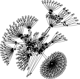
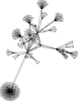
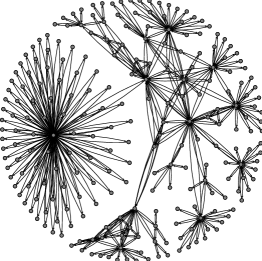
The most prominent representatives of spring layout are the Kamada-Kawai kamada89 and the Fruchterman-Reingold fruchterman91 algorithm. Figure 1 a and b show a complex heterogeneous network visualized with them. Several problems spring to mind: congestion, order less arrangement of nodes in the highly connected core and high variation in the edge length.

The contribution of this paper is first, to analyze the shortcomings of the spring model and second, to present a modified model that addresses these shortcomings. We will proceed as follows: First, we will formalize and analyze the spring model in its most general from. Having opened up the design space we propose changes to remedy the spring model’s defects. So, a new model will be derived from the general spring model. In the next section, an evaluation of the new model will be presented. This will be followed by several application examples in the field of complex systems. Finally concluding remarks will round up the discussion.

2 The Spring Model: A Critical View

For the following discussion we will assume a graph $G$ to be a tuple $G=(V,E)$ where $V$ is the set of vertices or nodes respectively and $E\subseteq V\times V$ is the set of edges. We will use the indices $i$ and $j$ to denote vertices. Whether the graph is directed or undirected is irrelevant for the discussion.

The general spring model is based on the idea that springs adjust the distances between connected nodes: connected nodes should be placed equidistantly. The spring pushes towards this desired distance $d$ which is the resting position of the spring. The force on $i$ of a spring between $i$ and $j$ is given as:

$$m\ddot{x}_{i}=K_{i,j}{(\|x_{j}-x_{i}\|-d)}{(x_{j}-x_{i})\over\|x_{j}-x_{i}\|}$$ (1)

$x_{i}$ is used to denote the position vector of node $i$. $K_{i,j}$ is the spring constant of the spring connecting $i$ and $j$. Thus $K$ is defined by:

$$K_{i,j}=\begin{cases}k,&\text{if $(i,j)\in E\lor(j,i)\in E$;}\\ 0,&\text{otherwise.}\end{cases}$$ (2)

As only connected nodes have springs between them each node is endowed with a repulsive field to adjust their distances. The resulting force experienced by $i$ in the presence of $j$ is thus:

$$m\ddot{x}_{i}=-\rho{(x_{j}-x_{i})\over\|x_{j}-x_{i}\|^{1+\beta}}$$ (3)

Assuming, that we mimic a Coulomb field, $\rho$ can be interpreted as the electrostatic constant multiplied by the charges of the two nodes. $\beta$ is commonly set to $2$.

Unfortunately, a system like this will start oscillating. Therefore friction is introduced:

$$m\ddot{x}_{i}=-\gamma\dot{x}$$ (4)

$\gamma$ denotes the friction constant.

Putting the forces together we get the following equation:

$$m\ddot{x}_{i}=-\gamma\dot{x}+\sum_{j\in V}K_{i,j}{(\|x_{j}-x_{i}\|-d)}{(x_{j}-x_{i})\over\|x_{j}-x_{i}\|}-\rho\sum_{j\in V}{(x_{j}-x_{i})\over\|x_{j}-x_{i}\|^{1+\beta}}$$ (5)

under the assumption that $m\ll\gamma,\rho,K$ and $\gamma=1$ we can derive the following approximation for the movement of the nodes.

$$\dot{x}_{i}=\sum_{j\in V}K_{i,j}{(\|x_{j}-x_{i}\|-d)}{(x_{j}-x_{i})\over\|x_{j}-x_{i}\|}-\rho\sum_{j\in V}{(x_{j}-x_{i})\over\|x_{j}-x_{i}\|^{1+\beta}}$$ (6)

Having presented the general formulas for spring layout we will take a look at the outcome. Figure 1a shows a network, visualized with the spring layout by Kamada and Kawai kamada89 as implemented in graphvis’ neato layouter. Figure 1b shows the same network, visualized with an alternative spring model proposed by Fruchterman and Raingold fruchterman91 (graphvis’ fdp layouter). We notice several problems: First, there is congestion around strongly connected nodes (center area and bottom right). To many nodes are crammed in too little space by a force too strong. Unfortunately, the strongly connected nodes are often the ones that are of special interest in network analysis. Second problem: the available layout space is used inefficiently: there are big empty spaces, while in the center some nodes are occluded by others in the case of figure 1a. An even distribution of nodes would moreover facilitate any labeling of nodes. For figure 1b the structure is clearer. However the star cluster is pushed too far off by its repulsive field. The one connecting spring is not sufficient to compensate the repulsion. This unbalance is especially distinct in networks with highly heterogeneously node degress such as the ones predominant in complex systems research. Finally, the layout does not show much symmetry or structure. Instead, especially in the center, leaves a rather chaotic impression. The self organizing forces do not seem strong enough to disentangle the network. However, for laying out dynamically changing graphs, this would be vital.

The basic problem is this: The different forces at work are not well tuned. In some situations, attraction is to strong, in others repulsion is too dominant.

3 A New Model

The new model centers around the principle of balancing two forces: An attractive and a repulsive one. We thus call it arf We search for forces, that better represent commonly accepted principles of graph design like the following ones fruchterman91 :

1. Vertices connected by an edge should be drawn near each other.

2. Vertices should not be drawn too close to each other.

The fact that“[…] the layout should display as much symmetry as possible” as noted by eades84 will be taken into account. We will address these issues by challenging assumptions made in the spring layout. In doing so, we will derive a new force model for laying out networks.

Let us first take a look at the spring force: Obviously, connected nodes should be close to each other for two reasons: First humans find it difficult to follow long edges. Thus, short ones make the graph more readable. Second the shorter an edge the lower the risk of crossing another one. Thus an attractive spring force between nodes makes perfect sense. But, all nodes of a graph should stay close together to ensure that they are evenly spread. This will avoid runaway clusters such as the one in figure 1 b because each repulsive connection between two nodes is now balanced by an attractive one. The new equation for the spring constant $K$ is defined as follows:

$$K_{i,j}=\begin{cases}0,&\text{if $i=j$;}\\ a,&\text{if $(i,j)\in E\lor(j,i)\in E$;}\\ 1,&\text{otherwise.}\end{cases}$$ (7)

The parameter $a$ gives the strength of springs between connected nodes. It has to be greater than one: $a>1$. The greater $a$, the clearer the separation of unconnected sub clusters.

As described in the previous section, the resting position $d$ reflects the desired edge length. The spring force can be both attractive and repulsive, depending on the position of the nodes. However, there is already a repulsive field: We have two possible repulsive forces. By setting $d=0$ in equation (1), we accomplish two things: First, we clearly separate the attractive and repulsive forces. A more straight forward force system is easier to tune. Second, we abandon the rule to enforce equal length edges which led to congestion around highly connected nodes. The new equation for the attractive force is simply

$$m\ddot{x}_{i}=\sum_{j\in(V\setminus i)}{K_{i,j}({x}_{j}-{x}_{i})}$$ (8)

.

Besides the concern to have connected nodes close together and edges to be short, also an equal distribution of nodes in the available layout space is desirable. Repulsive movement addresses this concern. The balance between attraction and repulsion regulates the edge length in a very flexible way. However, in the previous section we diagnosed a miss balance in the force system. Loosely connected clusters were driven away by too much repulsion and in highly connected clusters, repulsion was not strong enough to counter congestion. With the new function for $K$ we already addressed this issue. Yet, we can still improve by changing repulsion from a quadratically decaying force to a distance invariant one. This is done by choosing $\beta=0$. The following term is used to calculate repulsion:

$$m\ddot{x}_{i}=-\rho\sum_{j\in(V\setminus i)}{{{x}_{j}-{x}_{i}\over{\|{x}_{j}-{x}_{i}}\|}}$$ (9)

Next, we have to take into account changing graph sizes. The node density should be invariant, not the size of the layout space. To scale the layout space based on the number of nodes in the graph, the repulsive force is multiplied by $\sqrt{|V|}$. This is accomplished by defining

$$\rho=b\sqrt{|V|}$$ (10)

in equation (9). $b$ in equation (10) scales the radius of the layout space.

When combining the force equations (8), (9,10), and the friction we can derive the following movement approximation for the nodes:

$$\dot{x}_{i}=\sum_{j\in(V\setminus i)}(K_{i,j}-{b\sqrt{|V|}\over{\|{x}_{j}-{x}_{i}\|}})({x}_{j}-{x}_{i})$$ (11)

The equation always leads to a circular layout space for the graph which is also very convenient for generating animations as frame sizes are invariant. Node density can be adjusted with the parameter $b$ and the separation of unconnected nodes with the parameter $a$ in the equation for $K$. The complete layout procedure is given by algorithm (1).

Algorithm 1 ARF Layout($G(V,E)$)

1:repeat

2:     $error\leftarrow 0$

3:     for all $i\in V$ do

4:         $\dot{x}_{i}=\sum_{j\in(V\setminus i)}{(K_{i,j}+{b{\sqrt{|V|}}\over{\|{x}_{j}-{x}_{i}}\|})({x}_{j}-{x}_{i})}$

5:         ${x}_{i}\leftarrow{x}_{i}+\Delta t{\dot{x}}_{i}$

6:         $error\leftarrow error+|\dot{x}_{i}|$

7:     end for

8:until $error<\epsilon$

The update of the node-position takes place in line 5 of algorithm (1). The parameter $\Delta t$ adjusts the size of one time step and thus the precision of the numerical integration. The choice of $\Delta t$ is a tradeoff between speed and potential instability which can be addressed by making $\Delta t$ depending on $|\dot{x}_{i}|$. The whole update is repeated until the amount of changes in the graph drops beneath a certain threshold $\epsilon$.

4 Evaluation

In this section we provide an evaluation of the new layout rules. As there is no commonly accepted benchmark for network layout. The following evaluation cannot and does not attempt to provide hard evidence. It rather attempts to indicate advantages of the movement model in a clear cut situation: layout of small to medium size networks.

As reference point for comparisons, the layouters contained in the graphviz package were used. Graphviz is maintained by AT&T and probably the best currently available graph layout tool. It contains the following five layouters: dot gansner93 , neato kamada89 , circo Six99 ; kaufmann02 , twopi wills97 and fdp fruchterman91 . The following evaluation compares arf in respect to layout quality. Computational complexity is not the issue here. Suffice it to say that all kinds of force directed layouts reside in the same complexity class, which is assumed to be $O(|V|^{2})$.

When assessing layout quality, the following four criteria are commonly accepted:

1. minimal number of crossing edges

2. aesthetics of the layout

3. separation of clusters

4. usage of the available space

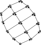
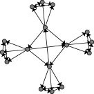
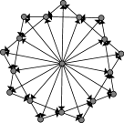
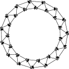
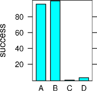
First, we will address points one and two: edge crossings and aesthetics. As the initial node positions are random, just looking at one generated layout is not enough. Thus, the following benchmark was used: The task is to lay out the four symmetrical graphs shown in figure 2 one hundred times.

A	B	C	D

arf	neato	ftp

Figure 2: Top: the four graphs (A,B,C and D) where used as benchmark. Bottom: Percent of successful layouts of each layouter for each of the benchmark graphs (number in percent).

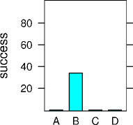
The layouts in the figure were produced by arf. Besides arf, the evaluation takes into account the layouters neato and fdp, both of which are probabilistic and force directed, too. The criteria for success are quite simple: For graphs A and D, each symetric layout without crossings is counted as success. For graphs B and C, no algorithm finds a crossing-free layout. So, all symetric layouts, that have no more crossings than the best produced layout, will be accepted. Figure 2 shows the results. It can be seen that arf applied to a random node distribution, in average, finds the optimal layout more often than neato and fdp, even though they use more sophisticated, non-incremental optimization algorithms. The only exception is the grid graph (A) where neato outperforms arf. For graphs C and D however, arf performs better. Please note that this benchmark only aims at small graphs. And the selection of only four graphs in not representative.

To address the points “separation of clusters” and “usage of the available space”, figure 3 shows an overview of layouts produced by arf and the graphviz layouters. The layouters were all called with the same input dot-file and without any further options. The first row shows the layout produced by arf. The other ones show the layouts produced by the different layouters in the graphviz package.

	E	F	G	H
arf
dot
neato
circo
twopi
fdp

Figure 3: Four different networks where visualized by various layouters: Arf, dot, neato, circo, twopi and fdp. The graphs can be characterized as follows: E is a network with two connected components and many unconnected nodes. F shows a scalefree network. G is a set of dentritic clusters. Finally H shows a random graph.

Right for the first graph (E), an advantage of arf can be seen: connected subgraphs are clearly separated, whereas in the layout produced by neato, twopi, and fdp, single nodes get “caught” in the “kite”-like subgraph. Looking at the layouts of graph (F) - a scale free network - the next column clearly shows arf’s ability to use the layout space economically can clearly be seen. Also for the dentritic clusters in graph (G), arf produces competitive results: The clusters are clearly separated and crossing free. Finally, arf produces a clearer and thus more readable layout for a random network (H). The nodes are more clearly arranged.

5 Application Examples

This section is devoted to the practical application of arf in the field of complex systems research. The first examples deals with the visualization of social network diagrams and auto catalytic networks. Next we show how state of the art animations can be generated in order to shed light on the dynamics of networks with changing structure. Finally, we highlight how the arf model can be fruitfully employed to explore large scale networks.

5.1 Autocatalytic and Social Networks

Crucial for interpreting networks is visualization that makes significant features easy to be perceived by the human eye. The following examples illustrate this.

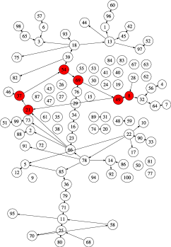
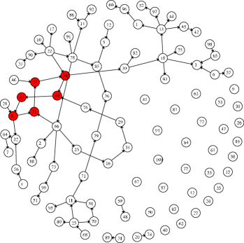
Figure 4 shows an autocatalytic network, taken from seufert06 . The network was laid out twice: The layout on the left is taken from the original publication (it was generated with twopi). The layout produced by arf (right) is far easier to read and to interpret: The networks contains one big connected component, three two-node-components and numerous single nodes. The connected component can be divided into a core forming an autocatalytic cycle (marked red) and a dentritic periphery. All these characteristic features are clearly visible in the right layout but not in the left one.

a	b

Figure 4: An auto catalytic network taken from seufert06 , laid out by twopi (a) and arf (b). Arf clearly shows the structural features of the graph: one big connected component with a dentritic periphery and a six-cycle (marked red).

Next we revisit the social network presented in section 1. In figure 1 managers of firms are connected by joint board membership. Sub figure 1 a and b are generated with neato and fdp. Sub figure 1 c was generated with arf. Even though the big star takes more space in c than in a and b, both the strongly connected core, as well as the periphery are given more space than in the other visualizations. Their structure is clearer and it is easier to discern different cliques of nodes.

5.2 Animating Dynamic Graphs

In this section we describe how arf can be used to produce state of the art animations. The basic scheme is shown in algorithm (2).

Algorithm 2 Animate($G$)

1:for all $c\in C$ do

2:     perform $c$ on $G$

3:     for $k$ times do

4:         relayout $G$

5:         render $G$

6:     end for

7:end for

In in the outer for loop, the algorithm iterates through all the changes $c$ in the set of changes $C$ that are to be performed to the graph $G$. These changes can, for example, be codified in a script:

addnode 12, addedge 12 1;
dropedge 12 1;

A similar script approach was also presented by brandes00 to codify and visualize changes in the WWW. This example would simultaneously add a node with id 12 and an edge from it to node 1. In the next graph change, the very same edge would be dropped. Now that the graph changed, the layout has to be adapted. This is done in $k$ steps to ensure a smooth transition from layout to layout. The smaller $k$, the faster the animation. The relayout procedure is just the body of the while-loop (lines 2-7) in Algorithm (1). After each relayout the graph is rendered to the screen or an image file, respectively.

In the latter case, the generated image files can easily be compiled to a video file of any format by using openly available graphics tools. Figure 5 shows an example of such an animation. Exactly the same procedure was used in actual research practice: The simulation of R&D cooperations between firms was animated with arf koenig06 . The videos can be downloaded at http://www.sg.ethz.ch/research/graphlayout/ as well as several other videos of evolving networks.

$t=0$	$t=90$	$t=180$	$t=270$	$t=360$
$t=450$	$t=540$	$t=630$	$t=720$	$t=810$

Figure 5: A dynamically changing graph laid out with arf.

5.3 Exploring Large Networks

Often networks are too large to be visualized completely. Just imagine cross-investment networks spanning entire countries or continents, the World Wide Web or our civilization’s social networks. In these cases, we can focus on only a small portion of the whole network at a given moment. The key concept is the one of a roving eye: There is one node in focus. Only this node and nodes within $n$ degrees of separation are shown and laid out. Of course we want to shift the focus interactively, for example by clicking on a node. The new node in focus defines a new set of visible nodes. Dynamic layout then gradually adjusts the positions of these nodes to generate a smooth transition from the old visualization to the new one.

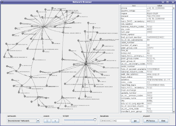
Essential for the responsiveness of the interaction are the properties of the applied movement model. The arf model was successfully employed to perform this task. Large databases containing network data can easily be explored. Figure 6 shows a snapshot. In the main window a section of the ownership network of Swiss firms is shown. On the right more detailed information on the focal node is presented.

Figure 6: A screen shot of the prototypical network browser. The left panel shows a part of the cross investment network of swiss firms, surrounding the retailer “COOP”. The right panel shows firm specific details.

6 Conclusion

This paper revisited the concept of force directed graph layout and put it into a complex systems context. An analysis of the classical spring model identified several deficiencies of the resulting layout. A new model was derived to resolve them. A model, especially suited for dynamic layout and the visualization of small ($n<10^{3}$) networks with strongly heterogeneous node degrees. The performance of the new model was evaluated and several successful applications in the field of complex systems research were discussed.

Demonstrations and videos can be found at http://www.sg.ethz.ch/research/graphlayout. A prototypical open source implementation of the new layouter is also available. It can easily be plugged into the open source graph library JUNG.

References

- [1] A.-L. Barabasi. Linked: How Everything Is Connected to Everything Else and What It Means. Plume, 2003.
- [2] U. Brandes, V. Kääb, A. Löh, D. Wagner, and T. Willhalm. Dynamic WWW structures in 3D. J. Graph Algorithms Appl, 4(3):183–191, 2000.
- [3] R. Davidson and D. Harel. Drawing graphs nicely using simulated annealing. ACM Transactions on Graphics, 15(4):301–331, Oct. 1996.
- [4] P. Eades. A heuristic for graph drawing. Congressus Numerantium, 42:149–160, 1984.
- [5] T. M. J. Fruchterman and E. M. Reingold. Graph drawing by force-directed placement. Softw. Pract. Exper., 21(11):1129–1164, 1991.
- [6] E. R. Gansner, E. Koutsofios, S. C. North, and K.-P. Vo. A technique for drawing directed graphs. Software Engineering, 19(3):214–230, 1993.
- [7] T. Kamada and S. Kawai. An algorithm for drawing general undirected graphs. Inf. Process. Lett., 31(1):7–15, 1989.
- [8] S. Kauffman. At Home in the Universe: The Search for the Laws of Self-Organization and Complexity. Oxford University Press, 1995.
- [9] M. Kaufmann and R. Wiese. Maintaining the mental map for circular drawings. In M. T. Goodrich and S. G. Kobourov, editors, Graph Drawing, Irvine, CA, USA, August 26-28, 2002, pages pp. 12–22. Springer, 2002.
- [10] M. König, S. Battiston, and F. Schweitzer. Microeconomic agent model of innovation networks. (to be submitted), 2006.
- [11] R. Mach and F. Schweitzer. Modeling vortex swarming in daphnia. Bulletin of Mathematical Biology, 69:539, 2007.
- [12] H. Meinhard. The Algorithmic Beauty of Sea Shell. Springer, 2003.
- [13] J. O’Madadhain, D. Fisher, P. Smyth, S. White, and Y.-B. Boey. Analysis and visualization of network data using JUNG. Journal of Statistical Software, 2005.
- [14] A. Quigley and P. Eades. FADE: Graph drawing, clustering, and visual abstraction. In GDRAWING: Conference on Graph Drawing (GD), 2000.
- [15] A. Seufert and F. Schweitzer. Aggregate dynamics in an evolutionary network model. International Journal of Modern Physics C, 2006.
- [16] J. M. Six and I. G. Tollis. A framework for circular drawings of networks. In Kratochv, editor, ”GDRAWING: Conference on Graph Drawing (GD)”, pages pp. 107–116. Springer, 1999.
- [17] S. H. Strogatz. Exploring complex networks. Nature, 410:268–276, 03 2001.
- [18] M. Veloso, P. Stone, and M. Bowling. Anticipation as a key for collaboration in a team of agents: A case study in robotic soccer. In P. S. Schenker and G. T. McKee, editors, Proceedings of SPIE Sensor Fusion and Decentralized Control in Robotic Systems II, volume 3839, pages 134–143, Bellingham, WA, September 1999. SPIE.
- [19] G. J. Wills. Nicheworks - interactive visualization of very large graphs. In GD ’97: Proceedings of the 5th International Symposium on Graph Drawing, pages 403–414, London, UK, 1997. Springer-Verlag.