Exploring the Variable Sky with the Sloan Digital Sky Survey
Abstract
We quantify the variability of faint unresolved optical sources using a catalog based on multiple SDSS imaging observations. The catalog covers SDSS Stripe 82, which lies along the celestial equator in the Southern Galactic Hemisphere (22h 24m 04h 08m, , deg2), and contains 58 million photometric observations in the SDSS system for 1.4 million unresolved sources that were observed at least 4 times in each of the bands (with a median of 10 observations obtained over 5 years). In each photometric bandpass we compute various low-order lightcurve statistics such as root-mean-square scatter (rms), per degree of freedom, skewness, minimum and maximum magnitude, and use them to select and study variable sources. We find that of unresolved optical sources brighter than appear variable at the 0.05 mag level (rms) simultaneously in the and bands. The majority (2/3) of these variable sources are low-redshift () quasars, although they represent only of all sources in the adopted flux-limited sample. We find that at least of quasars are variable at the 0.03 mag level (rms) and confirm that variability is as good a method for finding low-redshift quasars as is the UV excess color selection (at high Galactic latitudes). We analyze the distribution of lightcurve skewness for quasars and find that is centered on zero. We find that about 1/4 of the variable stars are RR Lyrae stars, and that only of stars from the main stellar locus are variable at the 0.05 mag level. The distribution of lightcurve skewness in the vs. color-color diagram on the main stellar locus is found to be bimodal (with one mode consistent with Algol-like behavior). Using over six hundred RR Lyrae stars, we demonstrate rich halo substructure out to distances of 100 kpc. We extrapolate these results to expected performance by the Large Synoptic Survey Telescope and estimate that it will obtain well-sampled accurate, multi-color lightcurves for million low-redshift quasars, and will discover at least 50 million variable stars.
1 Introduction
Variability is an important phenomenon in astrophysical studies of structure and evolution, both stellar and galactic. Some variable stars, such as RR Lyrae, are an excellent tool for studying the Galaxy. Being nearly standard candles (thus making distance determination relatively straightforward) and being intrinsically bright, they are a particularly suitable tracer of Galactic structure. In extragalactic astronomy, the optical continuum variability of quasars is utilized as an efficient method for their discovery (van den Bergh, Herbst & Pritchet, 1973; Hawkins, 1983; Koo, Kron & Cudworth, 1986; Hawkins & Veron, 1995), and is also frequently used to constrain the origin of their emission (Kawaguchi et al., 1998; Trevese et al., 2001; Martini & Schneider, 2003).
Despite the importance of variability, the variable optical sky remains largely unexplored and poorly quantified, especially at the faint end. To what degree different variable populations contribute to the overall variability, how they are distributed in magnitude and color, what the characteristic time-scales and the dominant mechanisms of variability are, are just some of the questions that still remain to be answered. To address these questions, several contemporary projects aimed at regular monitoring of the optical sky were started. Some of the more prominent surveys in terms of the sky coverage, depth, and cadence are:
-
•
The Faint Sky Variability Survey (Groot et al., 2003) is a very deep () survey of 23 deg2 of sky, containing about 80,000 sources sampled at timescales ranging from minutes to years.
-
•
The QUEST Survey (Vivas et al., 2001) monitors 700 deg2 of sky from to a limit of .
- •
- •
-
•
The MACHO Project monitored the brightness of million stars in deg2 of sky toward the Magellanic Clouds and the Galactic bulge for years to a limit of (Alcock et al., 2001).
A comprehensive review of past and ongoing variability surveys can be found in Becker et al. (2004).
Recognizing the outstanding importance of variable objects, the last Decadal Survey Report (Astronomy and Astrophysics Survey Committee, Board on Physics and Astronomy, Space Studies Board, National Research Council, 2001) highly recommended a major new initiative for studying the variable sky, the Large Synoptic Survey Telescope (LSST; Tyson et al. 2002; Walker 2003). The LSST111See [HREF]http://www.lsst.org will offer an unprecedented view of the faint variable sky: according to the current designs it will scan the entire accessible sky every three nights to a limit of with two observations per night in two different bands (selected from a set of six). One of the LSST science goals222For more details see [HREF]http://www.lsst.org/Science/science_goals.shtml will be the exploration of the transient optical sky: the discovery and analysis of rare and exotic objects (e.g. neutron star and black hole binaries), gamma-ray bursts, X-ray flashes, and of new classes of transients, such as binary mergers and stellar disruptions by black holes. The observed volume of space, and the requirement to recognize and monitor these events — in real time — on a “normally” variable sky, will present a challenge to the project.
Since LSST will utilize333LSST will also use the band at . For more details see the LSST Science Requirement Document at [HREF]http://www.lsst.org/Science/lsst_baseline.shtml the Sloan Digital Sky Survey (SDSS; York et al. 2000) photometric system (, Fukugita et al. 1996), multiple photometric observations obtained by the SDSS represent an excellent dataset for a pre-LSST study that characterizes the faint variable sky and quantifies the variable population and its distribution in magnitude-color-variability space. Here we present such a study of unresolved sources in a region that has been imaged multiple times by the SDSS.
In Section 2 we give a brief overview of the SDSS imaging survey and repeated scans of a deg2 region called Stripe 82. In Section 3, we describe methods used to select candidate variable sources from the SDSS Stripe 82 data assembled, averaged and recalibrated by Ivezić et al. (2007), and present tests that show the robustness of the adopted selection criteria. In the same section, we discuss the distribution of selected variable sources in magnitude-color-variability space. The Milky Way halo structure traced by selected candidate RR Lyrae stars is discussed in Section 4, and in Section 5 we estimate the fraction of variable quasars. Implications for surveys such as the LSST are discussed in Section 6, and our main results are summarized in Section 7.
2 Overview of the SDSS Imaging and Stripe 82 Data
The quality of photometry and astrometry, as well as the large area covered by the survey, make the SDSS stand out among available optical sky surveys (Sesar et al., 2006). The SDSS is providing homogeneous and deep () photometry in five bandpasses (, , , , and , Gunn et al. 1998; Hogg et al. 2002; Smith et al. 2002; Gunn et al. 2006; Tucker et al. 2006) accurate to 0.02 mag (root-mean-square scatter, hereafter rms) for unresolved sources not limited by photon statistics (Scranton et al., 2002; Ivezić et al., 2003a), and with a zeropoint uncertainty of 0.02 mag (Ivezić et al., 2004a). The survey sky coverage of 10,000 deg2 in the northern Galactic cap, and 300 deg2 in the southern Galactic cap will result in photometric measurements for well over 100 million stars and a similar number of galaxies (Stoughton et al., 2002). The recent Data Release 5 (Adelman-McCarthy et al., 2007)444Please see [HREF]http://www.sdss.org/dr5 lists photometric data for 215 million unique objects observed in 8000 deg2 of sky as part of the “SDSS-I” phase that ran through June 2005. Astrometric positions are accurate to better than per coordinate (rms) for sources with (Pier et al., 2003), and the morphological information from the images allows reliable star-galaxy separation to (Lupton et al., 2002). In addition, the 5-band SDSS photometry can be used for very detailed source classification; e.g. separation of quasars and stars (Richards et al., 2002), spectral classification of stars to within 1-2 spectral subtypes (Lenz et al., 1998; Finlator, 2000; Hawley et al., 2002), and even remarkably efficient color selection of the horizontal branch and RR Lyrae stars (Yanny et al., 2000; Sirko et al., 2004; Ivezić et al., 2005) and low-metallicity G and K giants (Helmi et al., 2003).
The equatorial Stripe 82 region (22h 24m 04h 08m, , deg2), observed in the southern Galactic cap, presents a valuable data source for variability studies. The region was repeatedly observed (65 imaging runs by July 2005, but not all cover the entire region), and it is the largest source of multi-epoch data in the SDSS-I phase. Another source of the large number of scans is the SDSS-II Supernova Survey (Frieman et al., 2007). By averaging the repeated observations of Stripe 82 sources, more accurate photometry than the nominal 0.02 mag single-scan accuracy can be achieved. This motivated Ivezić et al. (2007) to produce a catalog of recalibrated Stripe 82 observations. The catalog lists 58 million photometric observations for 1.4 million unresolved sources that were observed at least 4 times in each of the bands (with a median of 10 observations obtained over years). The random photometric errors for PSF (point spread function) magnitudes are below 0.01 mag for stars brighter than 19.5, 20.5, 20.5, 20, 18.5 in , respectively (about twice as accurate for individual SDSS runs), and the spatial variation of photometric zeropoints is not larger than 0.01 mag (rms). Following Ivezić et al. (2007), we use PSF magnitudes because they go deeper at a given signal-to-noise ratio than aperture magnitudes, and have more accurate photometric error estimates than model magnitudes. In addition, various low-order statistics such as root-mean-square scatter (), per degree of freedom (), lightcurve skewness (), minimum and maximum PSF magnitude, were computed for each band and each source. We compute per degree of freedom as
| (1) |
and lightcurve skewness as555We use equations from [HREF]http://www.xycoon.com/skewness_small_sample_test_1.htm.
| (2) |
| (3) |
| (4) |
where is the number of detections, is the magnitude, is the mean magnitude, and is the photometric error.
Separation of quasars and stars, as well as efficient color selection of horizontal branch and RR Lyrae stars, depend on accurate band photometry. To ensure this, we select 748,084 unresolved sources from the Ivezić et al. (2007) catalog with at least 4 detections in the band. A catalog of variable sources selected from this sample is analyzed in Section 3 below.
3 Analysis of Stripe 82 Catalog of Variable Sources
In this section we describe methods for selecting candidate variable sources, and present tests that show the robustness of the adopted selection criteria. The distribution of selected variable sources in magnitude-color-variability space is also presented.
3.1 Methods and Selection Criteria
Due to a relatively small number of observations per source and random sampling, we do not perform lightcurve fitting, but instead use low order statistics to select candidate variables and study their properties. There are four parameters (median PSF magnitude, root-mean-square scatter , , and lightcurve skewness ) measured in five photometric bands (, , , , and ), for a total of 20 parameters. In the analysis presented here, we utilize eight of them:
- •
-
•
and in the and bands, and
-
•
lightcurve skewness (the band combines a high signal-to-noise ratio and large variability amplitude for the majority of variable sources).
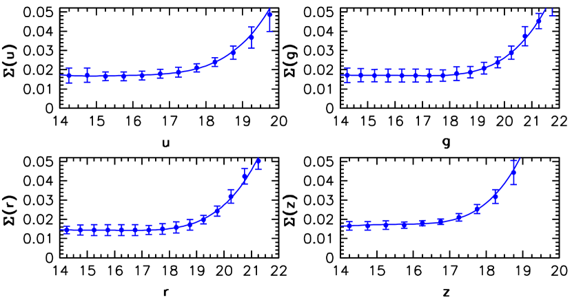
The observed root-mean-square scatter includes both the intrinsic variability and the mean photometric error as a function of magnitude. The dependence of on magnitude in the bands, is shown in Figure 1. For sources brighter than 18, 19.5, 19.5, 19, and 17.5 mag in the , respectively, the SDSS delivers photometry with little or no dependence on magnitude. We determine by fitting a fourth degree polynomial to median values in 0.5 mag wide bins (here we assume that the majority of sources are not variable). The theoretically expected function (Strateva et al., 2001)
| (5) |
provides equally good fits. We define the intrinsic variability (hereafter rms scatter ) as
| (6) |
for , and otherwise.
As the first variability selection criterion, we adopt mag and mag (hereafter written as mag). At the bright end, this criterion is equivalent to selecting sources with rms scatter greater than , where mag is the measurement noise. Selection cuts are applied simultaneously in the and bands to reduce the number of “false positives” (intrinsically non-variable sources selected as candidate variable sources due to measurement noise). About of sources pass the cut in each band separately, and of sources pass the cut in both bands simultaneously. By selecting sources with mag, we also select faint sources that have large due to large photometric errors at the faint end. To only select faint sources with statistically significant rms scatter, we apply the test as the second selection cut.
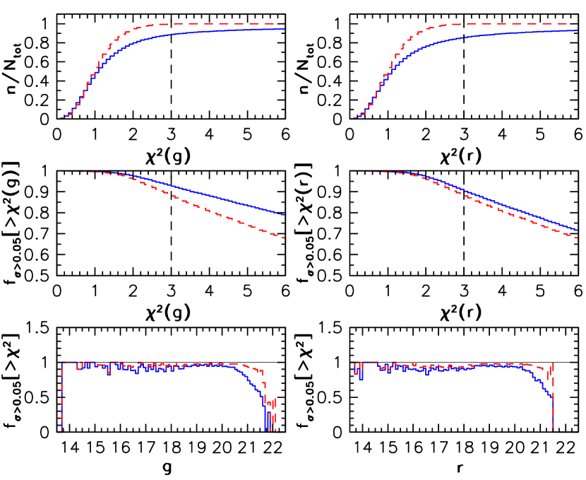
In the test, the value of per degree of freedom (calculated with respect to a weighted mean magnitude and using errors computed by the photometric pipeline) determines whether the observed lightcurve is consistent with the Gaussian distribution of errors. Large values show that the rms scatter is inconsistent with random fluctuations. Ivezić et al. (2003a, 2007) used multi-epoch SDSS observations to show that the photometric error distribution in the SDSS roughly follows a Gaussian distribution. A comparison of distributions in the and bands with a reference Gaussian distribution is shown in Figure 2. As evident, distributions in both bands roughly follow the reference Gaussian distribution for , demonstrating that median photometric errors are correctly determined. The discrepancy for larger is due to variable sources rather than non-Gaussian error distributions, as we demonstrate below.
The second selection cut, and (hereafter written as ), selects of mag sources, as shown in Figure 2 (middle panels). The effectiveness of the test is demonstrated in the bottom panel of Figure 2. For magnitudes fainter than , the fraction of candidate variables decreases as photometric errors increase. The selection is relatively uniform for sources brighter than , and we adopt this value as the flux limit for the selected variable sample.
There are 662,195 sources brighter than in the full sample. Using mag and as the selection criteria, we select 13,051 candidate variable sources666A list of candidate variable sources and their data from Ivezić et al. (2007) are publicly available from [HREF]http://www.sdss.org/dr5/products/value_added/index.html. Therefore, at least of unresolved optical sources brighter than appear variable at the mag level (rms) simultaneously in the and bands. The fraction of selected variable sources is not a strong function of the minimum required number of observations, but it does depend on the stellar density because the number of stars increases at lower Galactic latitudes (see Fig. 5 in Ivezić et al. 2007) while the quasar count remains the same.
3.2 The Counts of Variable Sources
In this section we estimate the completeness and efficiency of the candidate variable sample, and discuss the dependence of counts, rms scatter, ratio, and the lightcurve skewness on the position in the vs. color-color diagram.
3.2.1 Completeness
The selection completeness, defined as the fraction of true variable sources recovered by the algorithm, depends on the lightcurve shape and amplitudes. Due to a fairly large number of observations (median of 10), and small cutoff compared to typical amplitudes of variable sources (e.g. most RR Lyrae stars and quasars have peak-to-peak amplitudes mag), we expect the completeness to be fairly high for RR Lyrae stars (, see Section 4) and quasars (, see Section 5). The completeness for other types of variable sources, such as flares and eclipsing binaries, is hard to estimate, but is probably low due to sparse sampling.
3.2.2 Efficiency
The selection efficiency, defined as the fraction of true variable sources in the candidate variable sample, determines the robustness of the selection algorithm. The main diagnostic for the robustness of the adopted selection criteria is the distribution of selected candidates in the SDSS color-magnitude and color-color diagrams. The position of a source in these diagrams is a good proxy for its spectral classification (Lenz et al., 1998; Fan, 1999; Finlator, 2000; Smolčić et al., 2004).
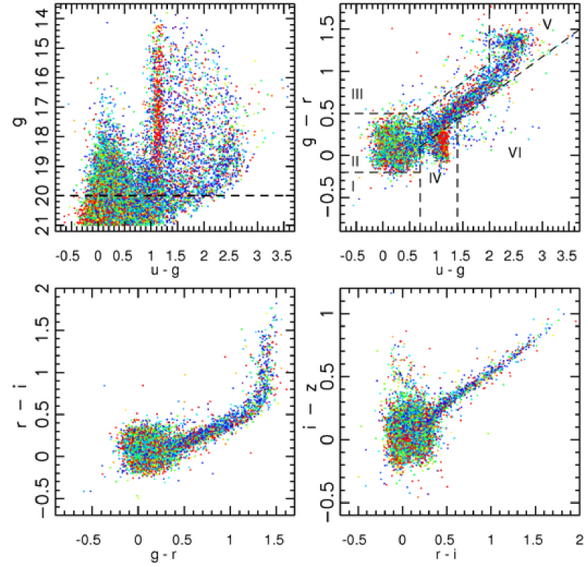
Figure 3 compares the distribution of candidate variable sources to that of all sources in the vs. color-color diagram. Were the selection a random process, the selected candidates would have the same distribution as the full sample. The distributions of candidate variables and of the full sample are remarkably different, demonstrating that the candidate variables are not randomly selected from the parent sample.
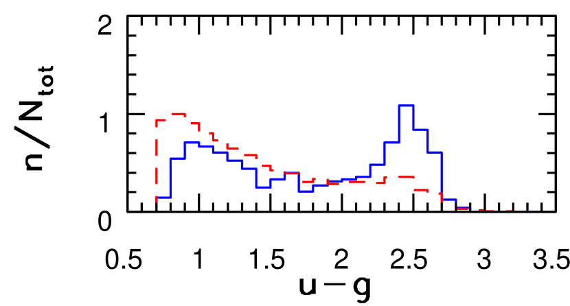
The three dominant classes of variable objects are quasars, RR Lyrae stars, and stars from the main stellar locus. The most obvious difference between the variable and the full sample distributions is a much higher fraction of low-redshift quasars (, recognized by their UV excess, , see Richards et al. 2002) and RR Lyrae stars (, , see Ivezić et al. 2005) in the variable sample, and vividly shown in the bottom panel of Figure 3.
Another interesting feature visible in this panel is a gradient in the fraction of variable main stellar locus stars (perpendicular to the main stellar locus). We investigate this gradient by first defining principal colors
| (7) |
and
| (8) |
where and are principal axis parallel and perpendicular to the main stellar locus, respectively (Ivezić et al., 2004a). The color is a measure of metallicity (Lenz et al., 1998), and stars are expected to be metal poor (Helmi et al., 2003). Sources with and are selected and binned in four bins. For each bin we calculate the fraction of source with mag, the fraction of variable sources (selected with mag and ), median , and the total number of sources in the bin (see Table 2). A greater fraction of variable sources in the last bin () indicates that, on average, metal-poor main stellar locus stars are more variable than the metal-rich stars. This could be because this sample of metal-poor stars is expected to have a high fraction of giants.
In order to quantify the differences between the full and the variable sample, we follow Sesar et al. (2006) and divide the vs. color-color diagram into six characteristic regions, each dominated by a particular type of source, as shown in Figure 4. The fractions and counts of variable and all sources in each region are listed in Table 1 for , , and flux-limited samples. Notably, in the adopted flux limit, the fraction of Region II sources (dominated by low-redshift quasars) in the variable sample is , or times greater than the fraction of Region II sources in the full sample (). The fraction of Region IV sources (which include RR Lyrae stars) in the variable sample is also high when compared to the full sample ( times higher).
As shown in Table 1, in the flux-limited sample, we find that low-redshift quasars and RR Lyrae stars (i.e. Regions II and IV) make of the variable population, while representing only of all sources. Quasars alone account for of the variable population. Stars from the main stellar locus represent of all sources and of the variable sample: about of the stars from the locus are variable at the mag level.
3.3 The Properties of Variable Sources
Various lightcurve properties, such as shape and amplitude, are expected to be correlated with stellar types. In this section we study the distribution of the rms scatter in the and bands, and ratio as a function of the and colors. To emphasize trends, we bin sources and present median values for each bin.
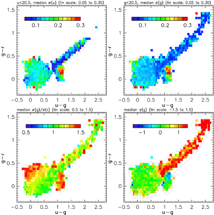
The distribution of the median and values in the vs. color-color diagram is shown in the top two panels of Figure 5. RR Lyrae stars show larger rms scatter ( mag) in the and bands, than low-redshift quasars or stars from the main stellar locus. Quasars also show slightly larger rms scatter in the band ( mag) than in the band ( mag), as discussed by Kinney et al. (1991),Ivezić et al. (2004b), and Vanden Berk et al. (2004). If we define the degree of variability as the root-mean-square scatter in the band, then on average RR Lyrae stars show the greatest variability, followed by quasars and the main stellar locus stars.
Another distinctive characteristic of variable sources is the ratio of flux changes in different bandpasses. This property can be used to select different types of variable sources. For example, RR Lyrae stars are bluer when brighter, a behavior used by Ivezić et al. (2000) to select RR Lyrae using 2-epoch SDSS data. Here we define a new parameter, , to express the ratio of flux changes in the and bands, and study its distribution in the vs. color-color diagram. In particular, we examine this distribution and its median values for three dominant classes of variable sources: quasars, RR Lyrae stars, and stars from the main stellar locus.
The bottom left panel in Figure 5 shows the distribution of median values as a function of and colors. Using Fig. 5 we note that on average:
-
•
RR Lyrae stars have
-
•
Main stellar locus stars have , and
-
•
Quasars show a gradient in the vs. color-color diagram.
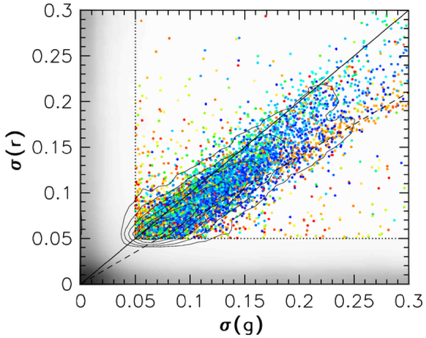
The average value of in Region IV indicates that RR Lyrae stars dominate the variable source count in this region. The ratio of 1.4 for RR Lyrae stars was also previously found by Ivezić et al. (2000). While Figure 5 only presents median values of the rms scatter, Figure 6 shows how the rms scatter in the and bands correlates with the color for individual sources. Variable sources that follow the relation also correlate with the color, and have , as expected for RR Lyrae stars.
The average ratio of (i.e. gray flux variations) for stars in the main stellar locus suggests that the variability could be caused by eclipsing systems. The distribution of for main stellar locus stars further strengthens this possibility, as discussed in Section 3.4 below.
The gradient in the ratio observed for low-redshift quasars in the vs. color-color diagram suggests that the variability correlation between the and bands is more complex than in the case of RR Lyrae or main stellar locus stars. Wilhite et al. (2006) show that the photometric color changes for quasars depend on the combined effects of continuum changes, emission-line changes, redshift, and the selection of photometric bandpasses. They note that due to the lack of variability of the lines, measured photometric color is not always bluer in brighter phases, but depends on redshift and the filters used. To verify the dependence of broad-band photometric variability on redshift, we plot vs. redshift for all spectroscopically confirmed unresolved quasars from Schneider et al. (2005) which are in Stripe 82, as shown in Figure 7. We confirm that the broad-band photometric variability depends on the redshift, and that the gradient in the vs. color-color diagram can be explained by the increase in from to in the 1.0 to 1.6 redshift range. This effect is due to the Mg II emission line (more stable in flux than the continuum) moving through the band filter over this redshift range. The implied correlation of the and colors with redshift is consistent with the discussion by Richards et al. (2002). The lack of noticeable correlation of with redshift is due to the combined effects of the dependence of on the rest-frame wavelength and time which cancel out (for a detailed model see Ivezić et al. 2004b).
3.4 Skewness as a Proxy for Dominant Variability Mechanism
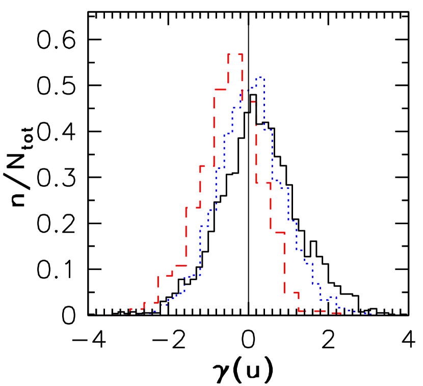
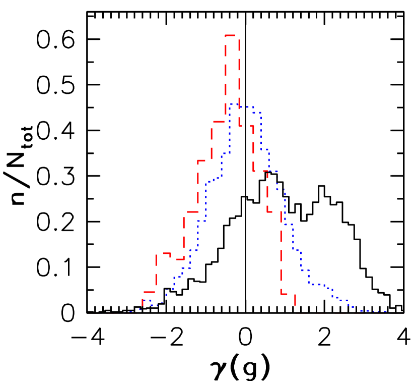
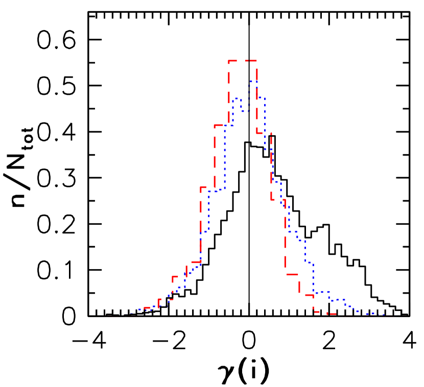
Lightcurve skewness, a measure of the lightcurve asymmetry, provides additional information on the type of variability. Negatively skewed, asymmetric lightcurves indicate variable sources that spend more time fainter than , where and are magnitudes at the minimum and maximum. Type RR Lyrae stars, for example, have negatively skewed lightcurves (, Wils, Lloyd & Bernhard 2006). Positively skewed, asymmetric lightcurves indicate variable sources that spend more time brighter than (e.g. eclipsing systems). Sources with symmetric lightcurves will have .
The bottom right panel in Figure 5 shows the distribution of the median as a function of the position in the vs. color-color diagram. On average, quasars and type RR Lyrae stars (, ) have , type RR Lyrae (, ) have negative skewness (), and stars in the main stellar locus have positive skewness.
Figure 8 shows the distribution of the lightcurve skewness in the bands for spectroscopically confirmed unresolved quasars from Schneider et al. (2005) which are in Stripe 82, candidate RR Lyrae stars (selection details are discussed in Section 4 below), and main stellar locus stars from our variable sample. Stars in the main stellar locus show a bimodal distribution. This distribution suggests at least two, and perhaps more, different populations of variables. Indeed, when spectroscopically confirmed M dwarfs are selected, a third peak appears at , possibly associated with flaring M dwarfs (Kowalski et al., 2007). The bimodality similar to the one in the band is also discernible in the band, while it is less pronounced in the band and not detected in the and bands (the and data are not shown).
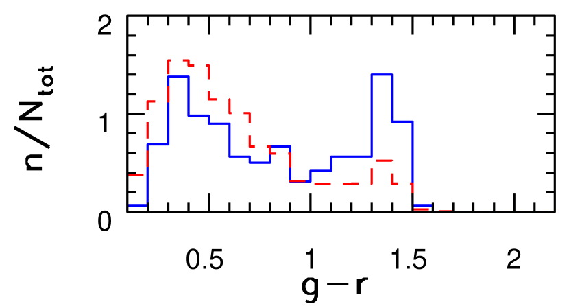
A comparison of the and color distributions for variable main stellar locus stars brighter than and a subset with highly asymmetric lightcurves () is shown in Figure 9. The subset with asymmetric lightcurves has an increased fraction of stars with colors and , that correspond to M stars. This may indicate that M stars have a higher probability of being associated with an eclipsing companion than stars with earlier spectral types. However, the selection effects are probably important since a companion is easier to detect (due to the low luminosity of M dwarfs). Kowalski et al. (2007) examine these issues using lightcurve data on a sample of spectroscopically confirmed M dwarfs. Finally, quasars have symmetric lightcurves () and their distribution of skewness does not change between bands.
4 The Milky Way Halo Structure Traced by Candidate RR Lyrae Stars
Studies of substructures in the Galactic halo, such as clumps and streams, can constrain the formation history of the Milky Way. One of the best tracers to study the outer halo are RR Lyrae stars because they are nearly standard candles, are sufficiently bright to be detected at large distances ( kpc for ), and are sufficiently numerous to trace the halo substructure with a high spatial resolution. The General Catalog of Variable Stars (GCVS; Kholopov et al. 1988) lists777A list of GCVS variability types can be found at [HREF]http://www.sai.msu.su/groups/cluster/gcvs/gcvs/iii/vartype.txt RR Lyrae stars as RR Lyrae type (RRab) and type (RRc) stars. RRab stars have asymmetric lightcurves, periods from 0.3 to 1.2 days, and amplitudes from to . RRc stars have nearly symmetric, sometimes sinusoidal, lightcurves, with periods from 0.2 to 0.5 days, and amplitudes not greater than . In this work we assume as the absolute band magnitude of RRab and RRc stars. A comprehensive review of RR Lyrae stars can be found in Smith (1995).
In this section we fine tune criteria for selecting candidate RR Lyrae stars, and estimate the selection completeness and efficiency. Using selected candidate RR Lyrae stars, we recover a known halo clump associated with the Sgr dwarf tidal stream, and find several new halo substructures.
4.1 Criteria for Selecting RR Lyrae Stars
Figures 3, 4, and 5 show that RR Lyrae stars occupy a well-defined region (Region IV) in the vs. color-color diagram, and Figure 6 shows how RR Lyrae stars follow the relation. Motivated by these results, we introduce color and cuts to specifically select candidate RR Lyrae stars from the variable sample, and study their distribution in the rms scatter-color-lightcurve skewness parameter space.
RR Lyrae stars have distinctive colors and can be selected with the following criteria (Ivezić et al., 2005):
| (9) |
| (10) |
| (11) |
| (12) |
| (13) |
where
| (14) |
and
| (15) |
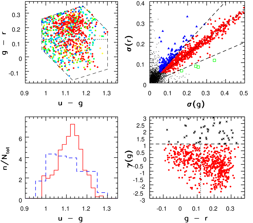
We apply these cuts to our sample of candidate variables and select 846 sources. It is implied by Ivezić et al. (2005) that RR Lyrae should always stay within these color boundaries, even though their colors change as a function of phase. Their distribution in the vs. color-color diagram and rms scatter in the band are shown in Figure 10 (top left panel). The distribution of sources in the RR Lyrae region is inhomogeneous. Sources with large rms scatter in the band ( mag) are centered around , and are separated by into two groups. A comparison with Figure 3 from Ivezić et al. (2005) suggests that these large rms scatter sources might be RR Lyrae type (RRab, ) and type stars (RRc, ). Small rms scatter sources ( mag) have a fairly uniform distribution, and are slightly bluer with .
The distribution of sources from the RR Lyrae region in the vs. diagram is presented in the top right panel of Figure 10. The majority of large rms scatter sources follow the relation, as expected for RR Lyrae stars. Since RR Lyrae stars are bluer when brighter, or equivalently, have greater rms scatter in the band than in the band, we require and select 683 candidate RR Lyrae stars.
A comparison of color distributions for candidate RR Lyrae stars and of sources with RR Lyrae colors, but not tagged as RR Lyrae stars, presented in the bottom left panel of Figure 10, demonstrates the robustness of the RR Lyrae selection. The two distributions are very different (the probability that they are the same is , as given by the KS test), with the candidate RR Lyrae distribution peaking at , as expected for RR Lyrae stars.
One property that distinguishes RRab from RRc stars is the shape (or skewness) of their lightcurves (in addition to lightcurve amplitude and period). RRab stars have asymmetric lightcurves, while RRc lightcurves are symmetric. In the top left panel of Figure 10, we noted that seemingly separates high rms scatter sources into two groups. If is the boundary between the RRab and RRc stars, then the same boundary should show up in the distribution of lightcurve skewness as a function of the color. As shown in Figure 10 (bottom left panel), this is indeed the case. On average, sources with have (symmetric lightcurves), as RRc stars, while sources have (asymmetric lightcurves) typical of RRab stars.
We show in Section 4.2 that candidate RR Lyrae stars with are contaminated by eclipsing variables. Therefore, to reduce the contamination by eclipsing variables, we also require , and select 634 sources as our final sample of candidate RR Lyrae stars.
4.2 Completeness and efficiency
The selection completeness, defined as the fraction of recovered RR Lyrae stars, will depend on the color cuts, cutoff, and the number of observations. The color cuts (Eqs. 9 to 15) applied in Section 4.1 were chosen to minimize contamination by sources other than RR Lyrae stars while maintaining an almost completeness (Ivezić et al., 2005). With the cutoff at 0.05 mag (small compared to the mag typical peak-to-peak amplitudes of RR Lyrae stars), and a fairly large number of observations per source (median of 10), we estimate the RR Lyrae selection completeness to be (see Appendix in Ivezić et al. 2000).
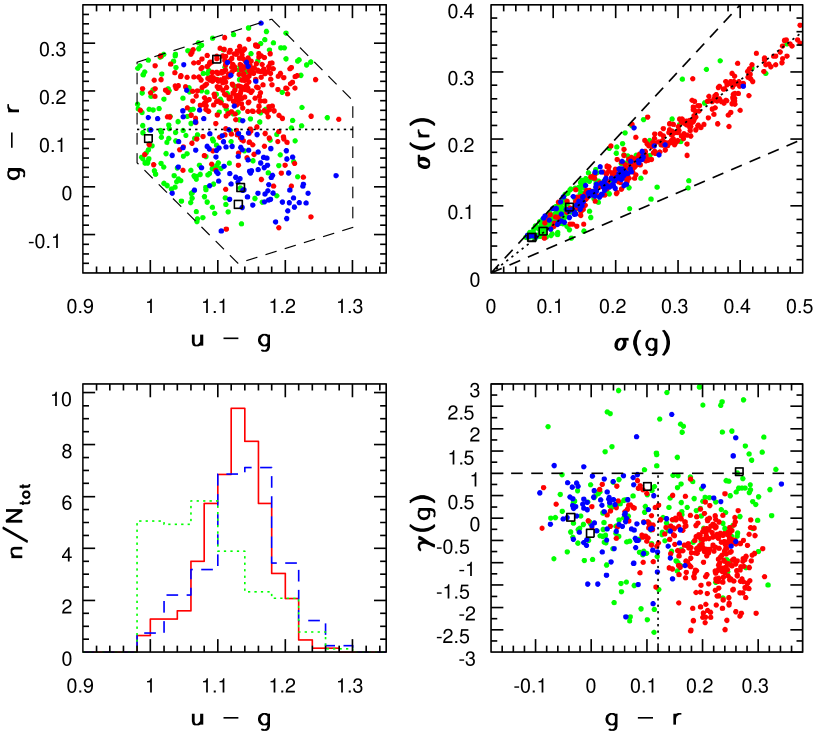
To determine the selection efficiency, defined as the fraction of true RR Lyrae stars in the RR Lyrae candidate sample, we positionally match 683 candidate RR Lyrae stars selected by to a sample of RR Lyrae sources selected from the SDSS Light-Motion-Curve Catalog (LMCC; Bramich et al. 2007). This catalog covers the same region of the sky as the one discussed here, but includes more recent SDSS-II observations that allow the construction of lightcurves. We match 613 candidates, while 70 candidate RR Lyrae stars from our sample, for some reason, do not have a match in the LMCC (De Lee, private communication). Following the classification based on phased lightcurves by De Lee et al. (2007), we find that of sources in our candidate RR Lyrae sample are classified as RRab and RRc, are classified as variable non-RR Lyrae stars, and only are spurious, non-variable sources. The most significant contamination comes from a population of variable sources bluer than (dotted line, bottom left panel Figure 11), possibly Population II Scuti stars, also known as SX Phoenicis stars (Hoffmeister, Richter & Wenzel, 1985).
The top left and the bottom right panels in Figure 11, show that RRab and RRc-dominated regions are separated by , as already hinted in Figure 10. Also, variable non-RR Lyrae sources with are classified by De Lee et al. (2007) as eclipsing variables, justifying our cut.
To summarize, using color criteria and criteria based on , , and RR Lyrae stars are selected with completeness and efficiency.
4.3 The Spatial Distribution of Candidate RR Lyrae Stars
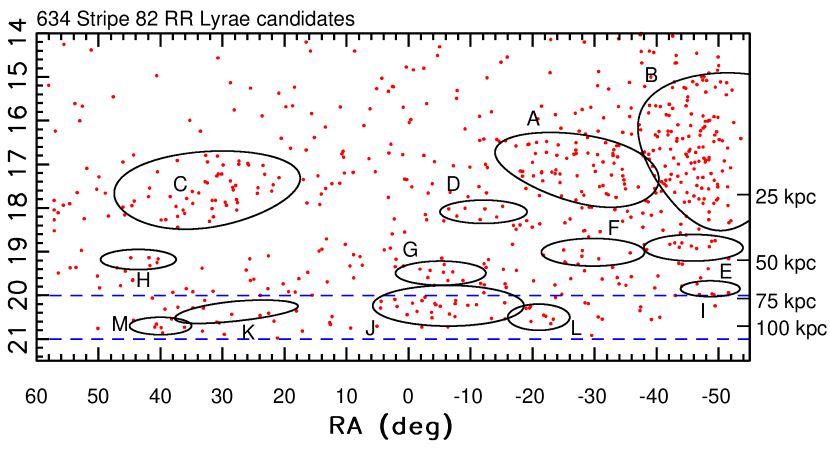
Using the selection criteria from Section 4.1 we isolate 634 RR Lyrae candidates. The magnitude-position diagram for these candidates within from the Celestial Equator is shown in Figure 12.
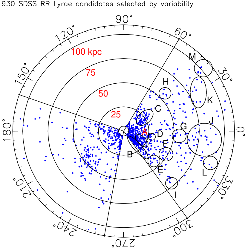
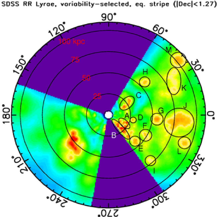
As discussed by Ivezić et al. (2005), an advantage of the data representation utilized in Figure 12 (magnitude–right ascension diagram) is its simplicity – only “raw” data are shown, without any post-processing. However, the magnitude scale is logarithmic and thus the spatial extent of structures is heavily distorted. In order to avoid these shortcomings, we have applied a Bayesian method for estimating continuous spatial density distribution developed by Ivezić et al. (2005) (see their Appendix B). The resulting density map is shown in the right panel in Figure 13. The advantage of that representation is that it better conveys the significance of various local overdensities. For comparison, we also show a map of the northern part of the equatorial strip constructed using 2-epoch data discussed by Ivezić et al. (2000).
We detect several new halo substructures at significance (compared to expected Poissonian fluctuations) and present their approximate locations and properties in Table 3. The most distant clump is at 100 kpc from the Galactic center. The strongest clump in the left wedge belongs to the Sgr dwarf tidal stream as does the clump marked by in the right wedge (Ivezić et al., 2003a). We note that the apparent “clumpiness” of the candidate RR Lyrae distribution increases with increasing radius, similar to CDM predictions by Bullock, Kravtsov & Weinberg (2001). A detailed comparison of their models with the data presented here will be discussed elsewhere (Sesar et al., in prep).
5 Are All Quasars Variable?
The optical continuum variability of quasars has been recognized since their first optical identification (Matthews & Sandage, 1963), and it has been proposed and utilized as an efficient method for their discovery (van den Bergh, Herbst & Pritchet, 1973; Hawkins, 1983; Koo, Kron & Cudworth, 1986; Hawkins & Veron, 1995). The observed characteristics of the variability of quasars are frequently used to constrain the origin of their emission (e.g. Kawaguchi et al. 1998 and references therein; Martini & Schneider 2003; Pereyra et al. 2006). Recently, significant progress in the description of quasar variability has been made by employing the SDSS data (de Vries, Becker & White, 2003; Ivezić et al., 2004b; Vanden Berk et al., 2004; de Vries et al., 2005; Sesar et al., 2006). Here we expand these studies by quantifying the efficiency of quasar discovery using variability.
A preliminary comparison of color and variability based methods for selecting quasars using SDSS data was presented by Ivezić et al. (2003b). They found that of spectroscopically confirmed unresolved quasars with UV excess have the band magnitude difference between two observations obtained two years apart larger than 0.15 mag. We can improve on their analysis because now there are significantly more observations obtained over a longer time period. Since quasars vary erratically and the rms scatter of their variability (the so-called structure function) increases with time (e.g. Vanden Berk et al. 2004 and references therein), the variability selection completeness is expected to be higher than obtained by Ivezić et al. (2003b).
First, although the adopted variability selection criteria discussed above are fairly conservative, we find that at least of low-redshift quasars are variable at the mag level (simultaneously in the and bands over observer’s time scales of several years) in the flux-limited sample. Second, even this estimate is only a lower limit: given the spectroscopic confirmation for a large flux-limited sample of quasars, it is possible to relax the adopted variability selection cutoff without a prohibitive contamination by non-variable sources.
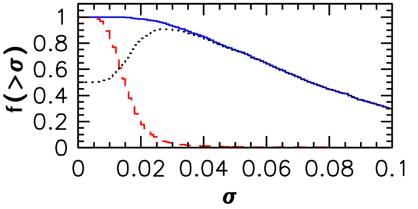
There are 2,492 unresolved quasars in the catalog of spectroscopically confirmed SDSS quasars (Schneider et al., 2005) from Stripe 82. The fraction of these objects that vary more than in the and bands, as a function of , is shown in Figure 14. We also show the analogous fraction for stars from the stellar locus. About of quasars vary with mag. For a small fraction of these objects the measured rms scatter is due to photometric noise, and the stellar data limit this fraction to be at most . Conservatively assuming that none of these of stars is intrinsically variable, we estimate that at least of quasars are variable at the 0.03 mag level on time scales up to several years.
6 Implications for Surveys such as LSST
The Large Synoptic Survey Telescope (LSST) is a proposed imaging survey that aims to obtain repeated multi-band imaging to faint limiting magnitudes over a large fraction of the sky. The LSST Science Requirement Document888 Available at [HREF]http://www.lsst.org/Science/lsst_baseline.shtml calls for repeated observations of a solid angle of deg2 distributed over the six photometric bandpasses and over 10 years. The results presented here can be extrapolated to estimate the lower limit on the number of variable sources that the LSST would discover.
The single-epoch LSST images will have a detection limit999An LSST Exposure Time Calculator is available at [HREF]www.lsst.org at . Hence, accurate photometry, comparable to the subsample with discussed here, will be available for stars with . The USNO-B catalog (Monet et al., 2003) shows that there are about stars with across the entire sky. About half of these stars are in the parts of the sky to be surveyed by the LSST. The simulations based on contemporary Milky Way models, such as those developed by Robin et al. (2003) and Jurić et al. (2007), predict that there are about twice as many stars with than with across the whole sky. Hence, it is expected that the LSST will detect about a billion stars with . This estimate is uncertain to within a factor of two or so due to unknown details in the spatial distribution of dust in the Galactic plane and towards the Galactic center.
We found that at least of stars from the main stellar locus can be detected as variable with photometry accurate to . This is only a lower limit because a much larger number of LSST observations obtained over a longer timespan than the SDSS data discussed here would increase this fraction. Hence, our results imply that the LSST will discover at least 50 million variable stars (without accounting for the fact that stellar counts greatly increase closer to the Galactic plane). Unlike the SDSS sample, where RR Lyrae stars account for of all variable stars, the number of RR Lyrae stars in the LSST sample will be negligible compared to other types of variable stars.
As estimated by Jurić et al. (2007) using deeper coadded SDSS photometry, there are about 100 deg-2 low-redshift quasars with (see also Beck-Winchatz & Anderson 2007 and references therein). Therefore, with a sky coverage of deg2, the LSST will obtain well-sampled accurate multi-color lightcurves for million low-redshift quasars. Even at the redshift limit of , this sample will be complete to , that is, almost to the formal quasar luminosity cutoff, and will represent an unprecedented sample for studying quasar physics.
7 Conclusions and Discussion
We have designed and tested algorithms for selecting candidate variable sources from a catalog based on multiple SDSS imaging observations. Using a sample of 13,051 selected candidate variable sources in the adopted flux-limited sample, we find that at least of unresolved optical sources appear variable at the mag level, simultaneously in the and bands. A similar fraction of variable sources () was also found by Sesar et al. (2006) using recalibrated photometric POSS and SDSS measurements, and by Morales-Rueda et al. (2006) using the Faint Sky Variability Survey data ().
Thanks to the multi-color nature of the SDSS photometry, and especially to the band data, we can obtain robust classification of selected variable sources. The majority (2/3) of variable sources are low-redshift () quasars, although they represent only of all sources in the adopted flux-limited sample. We find that about 1/4 of variable stars are RR Lyrae stars, and that only of stars from the main stellar locus are variable at the 0.05 mag level.
The distribution of for main stellar locus stars is bimodal, suggesting at least two, and perhaps more, different populations of variables. About a third of variable stars from the stellar locus show gray flux variations in the and bands (), and positive lightcurve skewness, suggesting variability caused by eclipsing systems. This population has an increased fraction of M type stars.
RR Lyrae stars show the largest rms scatter in the and bands, followed by low-redshift quasars. The ratio of rms scatter in the and bands for RR Lyrae is , in agreement with Ivezić et al. (2000) results based on 2-epoch photometry. The mean lightcurve skewness for RR Lyrae stars is , in agreement with Wils, Lloyd & Bernhard (2006). We selected a sample of 634 candidate RR Lyrae stars, with an estimated completeness and efficiency. Using these stars, we detected rich halo substructure out to distances of 100 kpc. The apparent “clumpiness” of the candidate RR Lyrae distribution increases with increasing radius, similar to CDM predictions by Bullock, Kravtsov & Weinberg (2001).
Low-redshift quasars show a dependence of on redshift, consistent with discussions in Richards et al. (2002) and Wilhite et al. (2006). The lightcurve skewness distribution for quasars is centered on zero in all photometric bands. We find that at least of quasars are variable at the 0.03 mag level (rms) on time scales up to several years. This confirms that variability is as a good a method for finding low-redshift quasars at high () Galactic latitudes as is the UV excess color selection. The fraction of variable quasars at the mag level obtained here (, see Figure 14) is comparable to 36% found by Rengstorf, Brunner & Wilhite (2006).
The multiple photometric observations obtained by the SDSS represent an excellent dataset for estimating the impact of surveys such as the LSST on studies of the variable sky. Our results indicate that the LSST will obtain well-sampled accurate multi-color lightcurves for million low-redshift quasars, and will discover at least 50 million variable stars. The number of variable stars discovered by the LSST will be of the same order as the number of all stars detected by the SDSS. With about 1000 data points in six photometric bands, it will be possible to recognize and classify variable objects using lightcurve moments of higher order than skewness discussed here, including lightcurve folding for periodic variables.
References
- Adelman-McCarthy et al. (2007) Adelman-McCarthy, J. K., Agüeros, M. A., Allam, S. S. et al., 2007, submitted
- Akerlof et al. (2000) Akerlof, C., Amrose, S., Balsano, R. et al., 2000, AJ, 119, 1901
- Alcock et al. (2001) Alcock, C., Allsman, R. A., Alves, D. R. et al., 2001, ApJS, 136, 439
- Astronomy and Astrophysics Survey Committee, Board on Physics and Astronomy, Space Studies Board, National Research Council (2001) Astronomy and Astrophysics Survey Committee, Board on Physics and Astronomy, Space Studies Board, National Research Council, 2001, Astronomy and Astrophysics in the New Millennium (The National Academies Press)
- Becker et al. (2004) Becker, A. C., Wittman, D. M., Boeshaar, P. C. et al., 2004, ApJ, 611, 418
- Beck-Winchatz & Anderson (2007) Beck-Winchatz, B., & Anderson, S. F., 2007, MNRAS, 374, 1506
- Bramich et al. (2007) Bramich, D. et al., 2007, in prep
- Bullock, Kravtsov & Weinberg (2001) Bullock, J. S., Kravtsov, A. V., & Weinberg D. H., 2001, ApJ, 548, 33
- De Lee et al. (2007) De Lee, N. et al., 2007, in prep
- de Vries, Becker & White (2003) de Vries, W. H., Becker, R. H., & White, R. L., 2003, AJ, 126, 1217
- de Vries et al. (2005) de Vries, W. H., Becker, R. H., White, R. L., & Loomis, C., 2005, AJ, 129, 615
- Fan (1999) Fan, X. 1999, AJ, 117, 2528
- Finlator (2000) Finlator, K., Ivezić, Ž., Fan, X. et al., 2000, AJ, 120, 2615
- Frieman et al. (2007) Frieman, J. A. et al., 2007, in prep
- Fukugita et al. (1996) Fukugita, M., Ichikawa, T., Gunn, J. E. et al., 1996, AJ, 111, 1748
- Groot et al. (2003) Groot, P. J., Vreeswijk, P. M., Huber, M. E. et al., 2003, MNRAS, 339, 427
- Gunn et al. (1998) Gunn, J. E., Carr, M., Rockosi, C. et al., 1998, AJ, 116, 3040
- Gunn et al. (2006) Gunn, J. E., Siegmund, W. A., Mannery, E. J. et al., 2006, AJ, 131, 2332
- Hawkins (1983) Hawkins, M. R. S., 1983, MNRAS, 202, 571
- Hawkins & Veron (1995) Hawkins, M. R. S., & Veron, P., 1995, MNRAS, 275, 1102
- Hawley et al. (2002) Hawley, S. L., Covey, K. R., Knapp, G. R. et al., 2002, AJ, 123, 3409
- Helmi et al. (2003) Helmi, A., Ivezić, Ž., Prada, F. et al., 2003, ApJ, 586, 195
- Hoffmeister, Richter & Wenzel (1985) Hoffmeister, C., Richter, G., & Wenzel, W., 1985, Variable Stars (New York:Springer)
- Hogg et al. (2002) Hogg, D. W., Finkbeiner, D. P., Schlegel, D. J. & Gunn, J.E., 2002, AJ, 122, 2129
- Ivezić et al. (2000) Ivezić, Ž., Goldston, J., Finlator, K. et al., 2000, AJ, 120, 963
- Ivezić et al. (2003a) Ivezić, Ž., Lupton, R. H., Anderson, S. et al., 2003a, Proceedings of the Workshop Variability with Wide Field Imagers, Mem. Soc. Astron. Italiana, 74, 978 (also astro-ph/0301400)
- Ivezić et al. (2003b) Ivezić, Ž., Lupton, R. H., Johnston, D. E. et al., 2003b, Proceedings of “AGN Physics with the SDSS”, Richards, G.T. & Hall, P.B., eds., in press (also astro-ph/0310566)
- Ivezić et al. (2004a) Ivezić, Ž., Lupton, R. H., Schlegel, D. et al., 2004a, Astronomische Nachrichten, 325, No. 6-8, 583-589 (also astro-ph/0410195)
- Ivezić et al. (2004b) Ivezić, Ž., Lupton, R. H., Jurić, M. et al., 2004b, Proceedings of “The Interplay among Black Holes, Stars, and ISM in Galactic Nuclei”, IAU Symposium No. 222, Bergmann, Th. S., Ho, L. C., & Schmitt, H. R., eds., p. 525 (also astro-ph/0404487)
- Ivezić et al. (2005) Ivezić, Ž., Vivas, A. K., Lupton, R. H. & Zinn, R., 2005, AJ, 129, 1096
- Ivezić et al. (2007) Ivezić, Ž., Smith, J. A., Miknaitis, G. et al., 2007, submitted to AJ (also astro-ph/0703157)
- Jurić et al. (2007) Jurić, M., Ivezić, Ž., Brooks, A. et al., 2007, submitted to AJ (also astro-ph/0510520)
- Kawaguchi et al. (1998) Kawaguchi, T., Mineshige, S., Umemura, M., & Turner, E. L., 1998, ApJ, 504, 671
- Kholopov et al. (1988) Kholopov, P. N., Samus, N. N., Frolov, M. S. et al., 1988, General Catalog of Variable Stars, 4th Ed. (Moscow:Nauka)
- Kinney et al. (1991) Kinney, A. L., Bohlin, R. C., Blades, J. C., & York, D. G., 1991, ApJS, 75, 645
- Koo, Kron & Cudworth (1986) Koo, D. C., Kron, R. G., & Cudworth, K. M., 1986, PASP, 98, 285
- Kowalski et al. (2007) Kowalski, A. et al, 2007, in prep
- Lenz et al. (1998) Lenz, D. D., Newberg, J., Rosner, R., Richards, G. T., & Stoughton, C., 1998, ApJS, 119, 121
- Lupton et al. (2002) Lupton, R. H., Ivezić, Ž., Gunn, J. E., Knapp, G. R., Strauss, M. A. & Yasuda, N., 2002, in “Survey and Other Telescope Technologies and Discoveries”, Tyson, J. A. & Wolff, S., eds. Proc. SPIE, 4836, 350
- Martini & Schneider (2003) Martini, P., & Schneider, D. P., 2003, ApJ, 597, L109
- Matthews & Sandage (1963) Matthews, T. A., & Sandage, A. R., 1963, ApJ, 138, 30
- McMillan & Herbst (1991) McMillan, J. D., & Herbst, W., 1991, AJ, 101, 1788
- Monet et al. (2003) Monet, D. G., Levine, S. E., Canzian, B. et al., 2003, AJ, 125, 984
- Morales-Rueda et al. (2006) Morales-Rueda, L., Groot, P. J., Augusteijn, T. et al., 2006, MNRAS, 371, 1681
- Pier et al. (2003) Pier, J. R., Munn, J. A., Hindsley, R. B., Hennesy, G. S., Kent, S. M., Lupton, R. H. & Ivezić, Ž., 2003, AJ, 125, 1559
- Pereyra et al. (2006) Pereyra, N. A., Vanden Berk, D. E., Turnshek, D. A., 2006, ApJ, 642, 87
- Richards et al. (2002) Richards, G. T., Fan, X., Newberg, H. J. et al., 2002, AJ, 123, 2945
- Rengstorf et al. (2004) Rengstorf, A. W., Mufson, S. L., Andrews, P. et al., 2004, AJ, 617, 184
- Rengstorf, Brunner & Wilhite (2006) Rengstorf, A. W., Brunner, R. J., & Wilhite, B. C., 2006, AJ, 131, 1923
- Robin et al. (2003) Robin, A. C., Reylé, C., Derriére, S., & Picaud, S., 2003, A&A, 409, 523
- Schlegel, Finkbeiner & Davis (1998) Schlegel, D., Finkbeiner, D. P., & Davis, M., 1998, ApJ500, 525
- Schneider et al. (2005) Schneider, D. P., Hall, P. B., Richards, G. T. et al, 2005, AJ, 367
- Scranton et al. (2002) Scranton, R., Scranton, R., Johnston, D. et al., 2002, ApJ, 579, 48
- Sesar et al. (2006) Sesar, B., Svilković, D., Ivezić, Ž. et al., 2006, AJ, 131, 2801
- Sirko et al. (2004) Sirko, E., Goodman, J., Knapp, G. et al., 2004, AJ, 127, 899S
- Smith (1995) Smith, H. A., 1995, RR Lyrae Stars (Cambridge University Press)
- Smith et al. (2002) Smith, J. A., Tucker, D. L., Kent, S. M. et al., 2002, AJ, 123, 2121
- Smolčić et al. (2004) Smolčić, V., Ivezić, Ž., Knapp, G. R. et al., 2004, ApJ, 615L, 141
- Strateva et al. (2001) Strateva, I., Ivezić, Ž., Knapp, G. R. et al., 2001, 122, 1861
- Tonry et al. (2005) Tonry, J. L., Howell, S. B., Everett, M. E. et al., 2005, PASP, 117, 281
- Stoughton et al. (2002) Stoughton, C., Lupton, R. H., Bernardi, M. et al., 2002, AJ, 123, 485
- Trevese et al. (2001) Trevese, D., Kron, R. G., & Bunone, A., 2001, ApJ, 551, 103
- Tucker et al. (2006) Tucker, D., Kent, S., Richmond, M. W. et al., 2006, Astronomische Nachrichten, 327, 821
- Tyson et al. (2002) Tyson, J.A., 2002, in “Survey and Other Telescope Technologies and Discoveries”, Tyson, J. A. & Wolff, S., eds. Proc. SPIE, 4836, 10
- Udalski et al. (2002) Udalski, A., Zebrun, K., Szymanski, M. et al., 2002, Acta Astron., 52, 115
- van den Bergh, Herbst & Pritchet (1973) van den Bergh, S., Herbst, E., & Pritchet, C. 1973, AJ, 78, 375
- Vanden Berk et al. (2004) Vanden Berk, D. E., Wilhite, B. C., Kron, R. G. et al., 2004, ApJ, 601, 692
- Vivas et al. (2001) Vivas, A. K., Zinn, R., Andrews, P. et al., 2001, ApJ, 554, L33
- Walker (2003) Walker, A.R., 2003, Proceedings of the Workshop Variability with Wide Field Imagers, Mem. Soc. Astron. Italiana, 74, 999 (also astro-ph/0303012)
- Wilhite et al. (2006) Wilhite, B. C., Vanden Berk, D. E., Kron, R. G. et al., 2006, ApJ, 633, 638
- Wils, Lloyd & Bernhard (2006) Wils, P., Lloyd, C., & Bernhard, K., 2006, MNRAS, 368, 1757
- Woźniak et al. (2002) Woźniak, P. R., Udalski, A., Szymanski, M. et al., 2002, Acta Astron., 52, 129
- Woźniak et al. (2004) Woźniak, P. R. et al., 2004, AJ127,2436
- Yanny et al. (2000) Yanny, B., Newberg, H. J., Kent, S. et al., 2000, ApJ, 540, 825
- York et al. (2000) York, D. G., Adelman, J., Anderson, S. et al., 2000, AJ, 120, 1579
- Żebruń et al. (2002) Żebruń, K., Soszyński, I., Woźniak, P. R. et al., 2002, Acta Astron., 51, 317
| Regiona | Nameb | % allc | % vard | var/alle | % allc | % vard | var/alle | % allc | % vard | var/alle | |||
|---|---|---|---|---|---|---|---|---|---|---|---|---|---|
| I | white dwarfs | 0.14 | 0.59 | 4.25 | 3.50 | 0.24 | 0.40 | 1.69 | 3.34 | 0.28 | 0.45 | 1.64 | 4.51 |
| II | low-redshift QSOs | 0.45 | 30.88 | 68.83 | 56.58 | 1.90 | 62.90 | 33.03 | 65.10 | 4.07 | 70.01 | 17.22 | 47.30 |
| III | dM/WD pairs | 0.08 | 0.53 | 6.54 | 5.37 | 0.83 | 2.08 | 2.50 | 4.92 | 1.21 | 3.79 | 3.13 | 8.61 |
| IV | RR Lyrae stars | 1.28 | 16.81 | 13.11 | 10.78 | 1.33 | 7.95 | 5.99 | 11.81 | 1.48 | 6.41 | 4.33 | 11.90 |
| V | stellar locus stars | 96.27 | 48.77 | 0.51 | 0.42 | 94.49 | 25.15 | 0.27 | 0.52 | 91.89 | 18.33 | 0.20 | 0.55 |
| VI | high-redshift QSOs | 1.78 | 2.42 | 1.36 | 1.12 | 1.21 | 1.52 | 1.26 | 2.48 | 1.07 | 1.01 | 0.95 | 2.60 |
| total count | 411,667 | 3,384 | 662,195 | 13,051 | 748,067 | 20,553 | |||||||
| Bin | % | % varb | Countsd | |
|---|---|---|---|---|
| 3.23 | 0.36 | 0.017 | 46,836 | |
| 2.92 | 0.28 | 0.017 | 136,910 | |
| 4.61 | 1.18 | 0.019 | 29,106 | |
| 11.50 | 4.10 | 0.027 | 4,547 |
| Labela | Nb | |||||||
|---|---|---|---|---|---|---|---|---|
| A | 84 | 330.95 | 21 | 17.02 | 1.14 | 0.18 | -0.50 | 0.62 |
| B | 144 | 309.47 | 22 | 16.76 | 1.12 | 0.16 | -0.57 | 0.64 |
| C | 54 | 33.69 | 25 | 17.61 | 1.13 | 0.20 | -0.68 | 0.29 |
| D | 8 | 347.91 | 29 | 18.02 | 1.14 | 0.23 | -0.50 | 0.38 |
| E | 11 | 314.06 | 43 | 18.84 | 1.09 | 0.20 | -0.41 | 0.75 |
| F | 11 | 330.26 | 48 | 19.16 | 1.07 | 0.20 | -0.46 | 0.38 |
| G | 10 | 354.81 | 55 | 19.46 | 1.10 | 0.22 | -0.69 | 0.38 |
| H | 7 | 43.57 | 57 | 19.32 | 1.05 | 0.04 | 0.06 | 1.34 |
| I | 4 | 311.34 | 72 | 19.98 | 1.08 | 0.11 | -0.10 | 2.0 |
| J | 26 | 353.58 | 81 | 20.21 | 1.11 | 0.20 | -0.27 | 0.58 |
| K | 8 | 28.39 | 84 | 20.35 | 1.10 | 0.20 | 0.14 | 0.44 |
| L | 3 | 339.01 | 92 | 20.45 | 1.06 | 0.16 | 0.08 | 0.67 |
| M | 5 | 39.45 | 102 | 20.73 | 1.07 | 0.11 | 0.36 | 1.67 |
