New varying speed of light theories

João Magueijo

The Blackett Laboratory,Imperial College of Science, Technology and Medicine

South Kensington, London SW7 2BZ, UK

ABSTRACT

We review recent work on the possibility of a varying speed of light (VSL). We start by discussing the physical meaning of a varying $c$, dispelling the myth that the constancy of $c$ is a matter of logical consistency. We then summarize the main VSL mechanisms proposed so far: hard breaking of Lorentz invariance; bimetric theories (where the speeds of gravity and light are not the same); locally Lorentz invariant VSL theories; theories exhibiting a color dependent speed of light; varying $c$ induced by extra dimensions (e.g. in the brane-world scenario); and field theories where VSL results from vacuum polarization or CPT violation. We show how VSL scenarios may solve the cosmological problems usually tackled by inflation, and also how they may produce a scale-invariant spectrum of Gaussian fluctuations, capable of explaining the WMAP data. We then review the connection between VSL and theories of quantum gravity, showing how “doubly special” relativity has emerged as a VSL effective model of quantum space-time, with observational implications for ultra high energy cosmic rays and gamma ray bursts. Some recent work on the physics of “black” holes and other compact objects in VSL theories is also described, highlighting phenomena associated with spatial (as opposed to temporal) variations in $c$. Finally we describe the observational status of the theory. The evidence is currently slim – redshift dependence in the atomic fine structure, anomalies with ultra high energy cosmic rays, and (to a much lesser extent) the acceleration of the universe and the WMAP data. The constraints (e.g. those arising from nucleosynthesis or geological bounds) are tight, but not insurmountable. We conclude with the observational predictions of the theory, and the prospects for its refutation or vindication.

j.magueijo@imperial.ac.uk

1 The black sheep of “varying-constant” theories

One field of work in which there has been too much speculation is cosmology. There are very few hard facts to go on, but theoretical workers have been busy constructing various models for the universe, based on any assumptions that they fancy. These models are probably all wrong. It is usually assumed that the laws of nature have always been the same as they are now. There is no justification for this. The laws may be changing, and in particular quantities which are considered to be constants of nature may be varying with cosmological time. Such variations would completely upset the model makers.

Paul Dirac, “On methods in theoretical physics”, June 1968, Trieste.

Since Dirac wrote these words in 1968, much has changed in our understanding of the universe. It is fair to say that cosmologists now have many “hard facts to go on”. They have mapped the cosmological expansion up to redshifts of order one [1, 2, 3, 4]. They have made high precision observations of the cosmic microwave background (CMB) [5, 6], a major asset to observational cosmology – and hardly an established fact in 1968. Big Bang nucleosynthesis has become a reasonably direct probe of the conditions in the universe one second after the Big Bang [7]. And there are many more: cosmologists can no longer indulge in mere flights of fancy. Cosmology has finally become an experimental science, or – some might say – a proper science.

And yet, any statement about the universe’s life before one second of age is still necessarily a speculation. No observational technique has so far penetrated this murky past, and Dirac’s views are still painfully applicable. In particular, it could well be that the constants of nature are not constant at all, but were varying significantly during this early phase. Assuming their constancy at all times requires massive extrapolation, with no observational basis. Could the universe come into being riding the back of wildly varying constants?

As Dirac’s quote shows, this question is far from new, and several “constants” of nature have been stripped off their status in theories proposed in the past. Physicists have long entertained the possibility of a varying gravitational constant $G$ [8, 9, 10], a varying electron charge $e$ [11], and more generally varying coupling constants. Indeed with the advent of string theory (and the prediction of the dilaton), to “vary” these “constants” seems to be fashionable.

In sharp contrast, the constancy of the speed of light has remain sacred, and the term “heresy” is occasionally used in relation to “varying speed of light theories” [12]. The reason is clear: the constancy of $c$, unlike the constancy of $G$ or $e$, is the pillar of special relativity and thus of modern physics. Varying $c$ theories are expected to cause much more structural damage to physics’ formalism than other varying constant theories.

Ironically, the first “varying-constant” was the speed of light, as suggested by Kelvin and Tait [13] in 1874. Some 30 years before Einstein’s proposal of special relativity, a varying c did not shock anyone, as indeed $c$ – unlike $G$ – played no special role in the formalism of physics. This is to be contrasted with the state of affairs after 1905, when Eddington would say: “A variation in c is self-contradictory”[14]. This astonishing statement does a disservice to the experimental testability and scientific respectability of the theory of relativity. In the words of Hertz, “what is due to experiment may always be rectified by experiment”.

In this review we describe how recent work has brought a varying speed of light (VSL) into the arenas of cosmology, quantum gravity and experiment/observation. As a cosmological model, VSL may be seen as a competitor to inflation, solving the cosmological problems and providing a theory of structure formation. As a theory of quantum gravity it may be seen as a phenomenological project, more modest in scope than string theory or loop quantum gravity, but already capable of making contact with experiment. On the observational front it’s still early days, but we could already have seen evidence for VSL.

But despite these many-layered developments, some scientists still question the logical consistency of varying the speed of light. It seems befitting to start this review by addressing this matter.

2 The meaning of a varying $c$

In discussing the physical meaning of a varying speed of light, I’m afraid that Eddington’s religious fervor is still with us [15, 16]. “To vary the speed of light is self-contradictory” has now been transmuted into “asking whether $c$ has varied over cosmic history is like asking whether the number of liters to the gallon has varied” [16]. The implication is that the constancy of the speed of light is a logical necessity, a definition that could not have been otherwise. This has to be naive. For centuries the constancy of the speed of light played no role in physics, and presumably physics did not start being logically consistent in 1905. Furthermore, the postulate of the constancy of $c$ in special relativity was prompted by experiments (including those leading to Maxwell’s theory) rather than issues of consistency. History alone suggests that the constancy (or otherwise) of the speed of light has to be more than a self-evident necessity.

2.1 The argument against a varying $c$

But let’s examine the scientific merits of such a view. The trouble arises because the attitude in [17, 16] (as opposed to that in [15]) is far from risible and is founded on a perfectly correct remark . The speed of light is a quantity with units (units of speed) and in a world without constants there is no a priori guarantee that meter sticks are the same at all points and that clocks spread throughout the universe are identical. Clearly if a dimensionless constant is observed to vary – such as the fine structure constant $\alpha=e^{2}/\hbar c$ – that fact is unambiguous. But if $\alpha$ is seen to vary, the units employed to quote physical measurements may also be expected to vary. A meter stick may elongate or contract and a clock tick faster or slower . Hence under a changing $\alpha$ there is no guarantee that units of length, time and mass are fixed, and discussing the variability or constancy of a parameter with dimensions – such as the speed of light – is necessarily circular and depends on the definition of units one has employed. This remark was clearly made by Bekenstein [11], who pointed out that the “observation” of a varying dimensional constant is at best a tautology, since it relies on the definition of a system of units. He stressed that the result of any experiment is necessarily dimensionless, because it’s the result of a ratio of two things with the same dimensions: what is being measured and the “unit” employed. Hence, when assessing the constancy or variability of constants, experiments are only sensitive to dimensionless combinations of constants. From a strict operational point of view it only makes sense to talk about varying dimensionless constants.

Seen from another angle [16, 15], even in a world where all seems to vary and nothing is constant, it is always possible to define units such that $c$ remains a constant. Consider for instance the current official definition of the meter: one takes the period of light from a certain atomic transition as the unit of time, then states that the meter is the distance travelled by light in a certain number of such periods. With these definitions it is clear that $c$ will always be a constant, a statement akin to saying that the speed of light is one light-year per year. One then does not need to perform any experiment to prove the constancy of the speed of light: it is built into the definition of the units and has become a tautology.

The argument is therefore double-tailed:

• A varying $c$ is tautological and is tied to the definition of a system of units.

• Units may always be defined so that $c$ becomes a constant.

It is not often pointed out that even though these arguments are invariably invoked to attack a varying $c$, they apply equally well to any other dimensional constant: $e$, $\hbar$, $G$, etc. For exactly the same reasons one may argue that the variability of these constants is tautological, or that units may always be defined so that the variability envisaged by the theory is undone. And yet varying $e$ and $G$ theories are widely accepted. Are dilaton and Brans-Dicke theories “self-contradictory” as well? Taken without prejudice, the arguments against a varying $c$ could destroy any varying constant theory.

2.2 The loophole

To fix ideas, we consider an observational example: Webb and collaborators [18, 19] have reported evidence for redshift dependence in $\alpha$. Since $\alpha$ is dimensionless it does not fall prey to the above arguments. But then the question arises: given these observations, which of $e$, $\hbar$, $c$, or a combination thereof is varying? Yet again, some authors are keen to point out that interpreting the Webb et al results as a varying $c$ is meaningless, due to the above arguments. They fail to notice that when they state that these results are not due to a varying $c$ (thus, being due to a varying $e$ or $\hbar$) they are making an equally meaningless statement, for exactly the same reasons ($e$ and $\hbar$ have dimensions).

If $\alpha$ is seen to vary one cannot say that all the dimensional parameters that make it up are constant. Something – $e$, $\hbar$, $c$, or a combination thereof – has to be varying. The choice amounts to fixing a system of units, but that choice has to be made.

A possible way to evade this argument is to say that physical theories should only refer to directly measurable dimensionless parameters [16], a view I label fundamentalism. This commendable view is, however, mere pub talk – no one has ever set up a theory in which only dimensionless parameters exist. At the end of the day, even if all dimensionless parameters were running wild, one would still want to set up quantum mechanics using Planck’s “constant”, or electrodynamics using the speed of light. Dimensional quantities would still play a role, something made more obvious by noting that if “constants” do vary then they’re just quantities like any other (like fields, or the length of my desk). And even under wildly varying constants, I would still want to know the length of my desk in meters, no matter how the meter is defined.

We need units and dimensional parameters to set up physics. Dimensional parameters or quantities are a necessary evil in physics. For the most part they are tautological and meaningless; still within the whole construction one gleans operationally meaningful statements, which are indeed dimensionless. But it’s easier to get there by means of constructions which are purely human conventions. These conventions amount to a prescription for defining units of mass, time, and length (and temperature if required). In the context of varying dimensionless constants, that choice translates into a statement on which dimensional constants are varying.

2.3 No subjectivism – the example of Newtonian mechanics

It would seem that we are falling into subjectivism, but that is not the case. The choice of units is never arbitrary or personal, once one specifies a given dynamics (via a Lagrangian or otherwise), which may then make predictions to be refuted or verified by experiment. One system of units invariably renders the presentation of the dynamics simpler than all others. Changing the units would not change the physical content of the theory, but would change its aspect. Typically one aspect is simple, and all others are ridiculously complicated. This unambiguously fixes the units to be used.

To give an example, there is a priori nothing wrong with using my pulse as the unit of time, and rephrasing physics in “egocentric” units. The physical content of such a theory would be the same — but we know that the laws of physics would look pretty weird, while being operationally the same. There would even be the illusion of seemingly new phenomena: for instance, every time I ran to catch a bus the speed of light would decrease. But nothing would be physically different, and according to the fundamentalist view, this description would be perfectly acceptable, or at least as meaningless as the conventional description.

Less preposterously, there was once a time when one might be tempted to define time by means of a pendulum, and rephrase Newtonian gravity by insisting that a pendulum clock is the “right” way to keep time. According to such a “pendular physics”, objects would be more rigid and the speed of light higher for observers on the Moon (since a pendulum clock would tick slower than the conventional Newtonian clocks). Newton’s laws would look much more complicated (except for the $1/r^{2}$ law), but the physical content of the theory would be the same. And yet Newton did not do this: he picked a more sensible system of units, one which rendered the law of inertia, the uniformity of time, and the conservation of energy valid.

As these examples show, the ability to formulate a theory (in this case Newtonian mechanics) often depends on choosing the right units. This is far from new, and has been discussed at length in the past. To cite Poincaré [20]: “If now it be supposed that another way of measuring time is adopted, the experiments of which Newton’s law is founded would nonetheless have the same meaning. Only the enunciation of the law would be different (…). So that the definition implicitly adopted (…) may be summed up thus: time should be so defined that the equations of mechanics may be as simple as possible. In other words, there is not one way of measuring time more true than another; that which is adopted is only more convenient.”

The implications of this statement are far reaching. Poincaré clearly implies that matters as fundamental as the uniformity of time, and by consequence the law of inertia and the theorem of energy conservation, are not provable by experiment. Experiment is dimensionless, but these statements “have units”, e.g. depend on the definition of the unit of time, which is nothing but a convention. And yet that definition is not a subjective choice. One particular unit of time – that which renders the laws of classical mechanics simple – objectively stands out.

2.4 A general definition of VSL

The above discussion has many parallels with VSL, as one final example shows. In classical electromagnetism the speed of light is only constant in vacuum, and it “varies” in dielectric media. This statement falls prey to all the criticism usually directed at VSL, namely that we could choose units such that the speed of light in dielectric media is a constant. As in the example given by Poincaré, no doubt you could do that; however such a convention would render the enunciation of Maxwell’s laws in dielectric media very complicated. Instead of simply replacing $c$ by $c_{0}/\sqrt{\epsilon}$, in “constant $c$” units one would need to add new terms in gradients and time derivatives of $\epsilon$ to Maxwell’s equations. Simplicity tells you that in this context you should not choose units in which the speed of light is a constant.

We are now ready to define varying speed of light. VSL theories are theories in which you find yourself in a situation like the one in the last example, regarding the speed of light in vacuum. They are theories in which the dynamics is rendered more simple if units are chosen in which $c$ is not constant. Typically this can be achieved if Lorentz invariance is broken, or if the usual tools employed in differential geometry become frame dependent. But the point is that we cannot discuss “VSL vs constant $c$” until a specific dynamics is proposed. One may then discover that varying $c$ units are preferable: in Section 4.2 we will give an explicit example (compare Eqns (24) and (25) with Eqns (26) and (27)).

To return to the issue of the meaning of the observed varying $\alpha$, we note that while observers concern themselves with dimensionless quantities, theorists need dimensional quantities to set up their theories. In order to set up a theory it may be more convenient to choose one system of units rather than any other. In dilaton theories, or variants thereof [25, 11, 26, 27, 28], the observed variations in $\alpha$ are attributed to $e$; VSL theories [29, 30, 31, 32, 33, 34, 35, 36] blame $c$ for this variation (and in some cases $\hbar$ too, see [35]). These choices are purely a matter of convenience, and one may change the units so as to convert a VSL theory into a constant $c$, varying $e$ theory; however such an operation is typically very contrived, with the resulting theory looking extremely complicated. Hence the dynamics associated with each varying $\alpha$ theory “chooses” the units to be used, on the grounds of convenience, and this choice fixes which combination of $e$, $c$ and $\hbar$ is assumed to vary.

The good news for experimentalists is that once this theoretical choice is made, the different theories typically lead to very different predictions. Dilaton theories, for instance, violate the weak equivalence principle, whereas many VSL theories do not [40, 37]. VSL theories often entail breaking Lorentz invariance, whereas dilaton theories do not. These differences have clear observational implications, for instance the STEP satellite could soon rule out the dilaton theories capable of explaining the Webb et al results [41]. Violations of Lorentz invariance, as we shall see, should also soon be observed - or not. We shall return to these matters in Section 8.

2.5 Dimensionless varying $c$

We conclude by noting that the above considerations apply to theories displaying space-time variations in the speed of light, and that there are theories for which a varying $c$ is a dimensionless statement . For instance $c$ may be color dependent (e.g. [42]). One may then take two light rays, measure their frequencies and speeds (in whatever units) and compute the ratios between the two frequencies and between the two speeds. Both ratios are dimensionless. If the latter is different from one when the former is also different from one, we have an example of varying speed of light which does not depend on the units employed. Another example is bimetric VSL [46, 49], for which the speed of the photon and graviton may differ. One may form the ratio between the speed of the photon and that of the graviton, to form a dimensionless quantity associated with a varying speed of light. 

3 An abridged catalogue of recent VSL theories

Even after the proposal of special relativity in 1905 many varying speed of light theories were considered, most notably by Einstein himself [21]. VSL was then rediscovered and forgotten on several occasions. For instance, in the 1930s VSL was used as an alternative explanation for the cosmological redshift [22, 23, 24] (these theories conflict with fine structure observations). None of these efforts relates to recent VSL theories, which are firmly entrenched in the successes (and remaining failures) of the hot big bang theory of the universe. In this sense the first “modern” VSL theory was J. W. Moffat’s ground breaking paper [29], where spontaneous symmetry breaking of Lorentz symmetry leads to VSL and an elegant solution to the horizon problem.

Since then there has been a growing literature on the subject, with several groups working on different aspects of VSL (for an early review see [38]). In this section I categorize the main implementations currently being considered, without trying to be exhaustive. All VSL theories conflict in one way or another with special relativity and here I shall use the type of insult directed at special relativity as my classification criterion for VSL theories.

Recall that special relativity is based upon two independent postulates - the relative nature of motion and the constancy of the speed of light. VSL theories do not need to violate the first of these postulates, but in practice one finds it hard to dispense with the second without destroying the first. This leads to our first criterion for differentiating the various proposals: do they honor the relative nature of motion?

Regarding the second postulate of special relativity, VSL theories behave in a variety of ways, all arising from a careful reading of the small print associated the constancy of $c$. Loosely this postulate means that $c$ is a constant, but more precisely it states that the speed of all massless particles is the same, regardless of their color (frequency), direction of motion, place and time, and regardless of the state of motion of observer or emitter. There is a large number of combinations in which these different aspects can be violated, explaining the large number of VSL theories put forward.

Bearing this in mind we can now distinguish the following VSL mechanisms.

3.1 Hard breaking of Lorentz symmetry

The most extreme model is that proposed in [30], and studied further in [31]. In this model both postulates of special relativity are violated: there is a preferred frame in physics (usually identified with the cosmological frame); the speed of light varies in time, although usually only in the very early Universe; and the time-translation invariance of physics is broken [43]. It describes a world where not only the matter content of the universe, but also the laws of physics evolve in time.

The basic dynamical postulate is that Einstein’s field equations are valid, with minimal coupling (i.e. with $c$ replaced by a field in the relevant equations) in this particular frame:

$$G_{\mu\nu}-g_{\mu\nu}\Lambda={\frac{8\pi G}{c^{4}}}T_{\mu\nu}.$$ (1)

This is inspired by the statement of Maxwell’s equations in dielectric media. The first strong assumption is that the field $c$ does not contribute to the stress-energy tensor (this may also be implemented in more conservative theories, e.g. [35]). More importantly, this postulate can only be true in one frame. There is still a metric, a connection, and curvature and Einstein “tensors”, to be evaluated in a given frame at constant $c$ (no extra terms in gradients of $c$, e.g. in the expression for the connection in terms of the metric). But they are tied to a preferred frame, and non-covariant extra terms in gradients of $c$ will appear in other frames. As pointed out by [44] this is no longer a geometric theory. Minimal coupling at the level of Einstein’s equations is at the heart of the model’s ability to solve the cosmological problems (as we shall see in Section 4).

It is debatable whether such a theory may derive from an action principle formulation. We could perform all variations at constant $c$ and require that ${\cal L}_{c}$ must not contain the metric explicitly. Unsurprisingly a hamiltonian formulation of this theory is preferable [33]. The preferred frame is given by a 4-vector $u^{\mu}$, and the metric can be written as

$$g_{\mu\nu}=h_{\mu\nu}-u_{\mu}u_{\nu}$$ (2)

with $h_{\mu\nu}u^{\mu}=0$ and $u_{\mu}^{\mu}=-1$. In a cosmological setting this frame is defined by the proper time and the conformal space coordinates which ensure that $K=0,\pm 1$. The Einstein equations derived from this action are more simply written using the Hamiltonian formalism, with a 3+1 split induced by vector $u^{\mu}$ (see for instance [45]). With a unit lapse and zero shift (temporal gauge), the Hamiltonian density in Einstein’s theory takes the form

$${\cal H}=h^{1/2}{\left[-^{(3)}R+h^{-1}{\left(\Pi^{ij}\Pi_{ij}-{\frac{1}{2}}\Pi^{2}\right)}\right]}$$ (3)

(with $i,j=1,2,3$). The second fundamental form is given by

$$\kappa_{ij}={1\over c}{\frac{{\dot{h}_{ij}}}{2}}$$ (4)

and the momenta conjugate to the $h_{ij}$ are given by

$$\Pi_{ij}={\frac{\partial{\cal L}}{\partial{\dot{h}}^{ij}}}=h^{1/2}(\kappa_{ij}-\kappa h_{ij}).$$ (5)

The Hamiltonian constraint is ${\cal H}=0$ and the momentum constraint is

$$\nabla_{i}(h^{-1/2}\Pi^{ij})=0$$ (6)

The dynamical equations are

$${1\over c}{\dot{h}}_{ij}=2h^{-1/2}{\left(\Pi_{ij}-{\frac{1}{2}}h_{ij}\Pi\right)}$$ (7)

and

$${1\over c^{2}}{{\sqrt{h}}\over 2}[\dot{h}_{ij}-\dot{h}h_{ij}]\,\dot{} = -h^{1/2}{\left({}^{(3)}R_{ij}-{\frac{1}{2}}h_{ij}\,^{(3)}R\right)}$$ (8)

$$\ +{\frac{1}{2}}h^{-1/2}h_{ij}{\left(\Pi_{kl}\Pi^{kl}-{\frac{1}{2}}\Pi^{2}\right)}$$

$$\ -2h^{-1/2}{\left(\Pi_{i}^{k}\Pi_{kj}-{\frac{1}{2}}\Pi\Pi_{ij}\right)}$$

These are Einstein’s equations in vacuum, but an adaptation to include matter is easy to write down. These equations differ considerably when written in units in which $c$ does not vary, losing their minimal coupling aspect [33]. This is reminiscent of Maxwell’s equations in dielectric media if rewritten in units in which the speed of light in these media is a constant (we will give an example in Section 4.2). They also look considerably different in a different frame, signaling the breakdown of covariance. Indeed it is easy to show that these theories do not satisfy Bianchi identities [44]. Although in the initial model the speed of light, like the preferred frame $u^{\mu}$, was preset (and thus to be seen as a law of physics), this need not be the case. In Section 4 we shall show how a dynamical equation for $c$ may also be included in this formalism.

Other theories with a preferred frame $u^{\mu}$ have been considered in the past, e.g. the “aether theory” of [71], or the CPT-odd theory of Coleman and Glashow [47] (check out the 4-vector $s^{\mu}$ in their Eqn. (6)).

3.2 Bimetric VSL theories

This approach was initially proposed by J. W. Moffat and M. A. Clayton [46], and by I. Drummond [49]. In contrast with the above formulation, one does not sacrifice the first principle of special relativity and special care is taken with the damage caused to the second. In these theories the speeds of the various massless species may be different, but special relativity is still realized within each sector. Typically the speed of the graviton is taken to be different from that of massless matter particles. This is implemented by introducing two metrics (or tetrads in the formalism of [49, 50]), one for gravity and one for matter. The model was further studied by [54] (scalar-tensor model), [53] (vector model), and [35, 44, 55].

We now sketch an implementation of the scalar-tensor model. It uses a scalar field $\phi$ that is minimally coupled to a gravitational field described by the metric $g_{\mu\nu}$. However the matter couples to a different metric, given by:

$$\hat{g}_{\mu\nu}=g_{\mu\nu}+B\partial_{\mu}\phi\partial_{\nu}\phi.$$ (9)

Thus there is a space-time, or graviton metric $g_{\mu\nu}$, and a matter metric $\hat{g}_{\mu\nu}$. The total action is:

$$S=S_{g}+S_{\phi}+\hat{S}_{\rm M},$$ (10)

where the gravitational action is as usual

$$S_{g}=-\frac{c^{4}}{16\pi G}\int dx^{4}{\sqrt{-g}}(R(g)+2\Lambda),$$ (11)

(notice that the cosmological constant $\Lambda$ could also, non-equivalently, appear as part of the matter action). The scalar field action is:

$$S_{\phi}=\frac{c^{4}}{16\pi G}\int dx^{4}{\sqrt{-g}}\,\Bigl{[}\frac{1}{2}g^{\mu\nu}\partial_{\mu}\phi\partial_{\nu}\phi-V(\phi)\Bigr{]},$$ (12)

leading to the the stress-energy tensor:

$$T^{\mu\nu}_{\phi}=\frac{c^{4}}{16\pi G}\Bigl{[}g^{\mu\alpha}g^{\nu\beta}\partial_{\alpha}\phi\partial_{\beta}\phi-\frac{1}{2}g^{\mu\nu}g^{\alpha\beta}\partial_{\alpha}\phi\partial_{\beta}\phi+g^{\mu\nu}V(\phi)\Bigr{]}.$$ (13)

The matter action is then written as usual, but using the metric ${\hat{g}}_{\mu\nu}$. Variation with respect to $g_{\mu\nu}$ leads to the gravitational field equations:

$$G^{\mu\nu}=\Lambda g^{\mu\nu}+\frac{8\pi G}{c^{4}}T^{\mu\nu}_{\phi}+\frac{8\pi G}{c^{4}}\frac{\sqrt{-\hat{g}}}{\sqrt{-g}}\hat{T}^{\mu\nu}.$$ (14)

In this theory the speed of light is not preset, but becomes a dynamical variable predicted by a special wave equation

$$\bar{g}^{\mu\nu}\hat{\nabla}_{\mu}\hat{\nabla}_{\nu}\phi+KV^{\prime}[\phi]=0\,$$ (15)

where the biscalar metric $\bar{g}$ is defined in [46].

This model not only predicts a varying speed of light (if the speed of the graviton is assumed to be constant), but also allows solutions with a de Sitter phase that provides sufficient inflation to solve the horizon and flatness problems. This is achieved without the addition of a potential for the scalar field. The model has also been used as an alternative explanation for the dark matter [50] and dark energy[44, 55]. In Section 5 we shall describe the implications of this model for structure formation.

3.3 Color-dependent speed of light

This approach may or may not preserve the first postulate of special relativity, the relative nature of motion; however, it generally violates its second postulate in the sense that the speed of light is allowed to vary with color (typically only close to the Planck frequency). This is achieved by deforming the photon dispersion relations $E^{2}-p^{2}=m^{2}=0$. For instance, it was proposed that:

$$E^{2}=p^{2}+m^{2}+\lambda E^{3}+...$$ (16)

where $\lambda$ is of the order of the Planck length. If this dispersion relation is true in one frame, and if the linear Lorentz transformations are still valid, then they are not true in any other frame, and so this theory – like that of [30] described in Section 3.1 – contradicts the principle of relativity. This is the case in the pioneering work in [56, 57, 58] where the effect was found for space-time foam. However this need not be the case [59, 60, 67]. One may preserve full Lorentz invariance (with a non-linear realization) and still accommodate deformed dispersion relations.

Under deformed dispersion relations, the group velocity of light, $c=dE/dp$, acquires an energy dependence. Such a dependence could be observed in planned gamma ray observations [56]. An energy dependent speed of light may also imply that the speed of light was faster in the very early universe, when the average energy was comparable to Planck energies [64]. This may be used to implement VSL cosmology and even inflation [65]. Such theories make viable predictions for structure formation [66], as explained further in Section 5. Finally a modified dispersion relation may lead to an explanation of the dark energy, in terms of energy trapped in very high momentum and low-energy quanta, as pointed out by [62].

But these theories are popular mainly as phenomenological descriptions of quantum gravity (e.g. [67, 68]) and as an explanation for the threshold anomalies (e.g. [69, 68]). We will describe these aspects in more detail in Section 6.

3.4 “Lorentz invariant” VSL theories

It is also possible to preserve the essence of Lorentz invariance in its totality and still have a space-time (as opposed to energy dependent) varying $c$. One possibility is that Lorentz invariance is spontaneously broken, as proposed by J. W. Moffat in his seminal paper [29, 70] (see also [71]). Here the full theory is endowed with exact local Lorentz symmetry; however the vacuum fails to exhibit this symmetry. For example an $O(3,1)$ scalar field $\phi^{a}$ (with $a=0,1,2,3$) could acquire a time-like vacuum expectation value (vev), providing a preferred frame and spontaneously breaking local Lorentz invariance to $O(3)$ (rotational invariance). Such a vev would act as the preferred vector $u^{a}=\phi^{a}_{0}$ used in Section 3.1; however the full theory would still be locally Lorentz invariant. Typically in this scenario the speed of light undergoes a first or second order phase transition to a value more than 30 orders of magnitude smaller, corresponding to the presently measured speed of light. Interestingly, before the phase transition the entropy of the universe is reduced by many orders of magnitude, but afterwards the radiation density and entropy of the universe vastly increase. Thus the entropy increase follows the arrow of time determined by the spontaneously broken direction of the timelike vev $\phi^{a}_{0}$. This solves the enigma of the arrow of time and the second law of thermodynamics (we will discuss the implications of this work for quantum cosmology later).

Another example is the covariant and locally Lorentz invariant theory proposed in [35]. In that work definitions were proposed for covariance and local Lorentz invariance that remain applicable when the speed of light $c$ is allowed to vary. They have the merit of retaining only those aspects of the usual definitions which are invariant under unit transformations, and which can therefore legitimately represent the outcome of an experiment (see discussion in Section 2 above). In the simplest case a scalar field is then defined $\psi=\log(c/c_{0})$, and minimal coupling to matter requires that

$$\alpha_{i}\propto g_{i}\propto\hbar c\propto c^{q}$$ (17)

with $q$ a parameter of the theory. The action may be taken to be

$$S=\int d^{4}x\sqrt{-g}(e^{a\psi}(R-2\Lambda+{\cal L}_{\psi})+{16\pi G\over c_{0}^{4}}e^{b\psi}{\cal L}_{m})$$ (18)

and the simplest dynamics for $\psi$ derives from:

$${\cal L}_{\psi}=-\kappa(\psi)\nabla_{\mu}\psi\nabla^{\mu}\psi$$ (19)

where $\kappa(\psi)$ is a dimensionless coupling function. For $a=4$, $b=0$, this theory is nothing but a unit transformation applied to Brans-Dicke theory. More generally, it’s only when $b+q=0$ that these theories are scalar-tensor theories in disguise. In all other cases it has been shown that a unit transformation may always be found such that $c$ is a constant but then the dynamics of the theory becomes much more complicated (see discussion in Section 2).

In these theories the cosmological constant $\Lambda$ may depend on $c$, and so act as a potential driving $\psi$. Since the vacuum energy usually scales like $c^{4}$ we may take $\Lambda\propto(c/c_{0})^{n}=e^{n\psi}$ with $n$ an integer. In this case, if we set $a=b=0$ the dynamical equation for $\psi$ is :

$$\Box\psi={32\pi G\over c^{4}\kappa}{\cal L}_{m}+{1\over\kappa}n\Lambda$$ (20)

Thus it is possible, in such theories, that the presence of Lambda drives changes in the speed of light, a matter examined (in another context) in [72].

Particle production and second quantization for this model has been discussed in [35]. Black hole solutions were also extensively studied [75], and some results will be summarized in Section 7. Predictions for the classical tests of relativity (gravitational light deflection, gravitational redshift, radar echo delay, and the precession of the perihelion of Mercury) were also shown to differ distinctly from their Einstein counterparts, while still evading experimental constraints [75]. Other interesting results were the discovery of Fock-Lorentz space-time[80, 81] as the “free” solution, and fast-tracks (tubes where the speed of light is much higher) as solutions driven by cosmic strings [35].

Beautiful as these two theories may be, their application to cosmology is somewhat cumbersome.

3.5 String/M-theory efforts

This line of VSL work was initiated by Kiritis [73] and Alexander [74], and makes use of the brane-world scenario, in which our Universe is confined to a 3-brane living in a space with a larger number of dimensions (the bulk). They found that if the brane lives in the vicinity of a black hole it is possible to have exact Lorentz invariance (and hence a constant speed of light in the bulk) while realizing VSL on the brane. In this approach VSL results from a projection effect, and the Lorentz invariance of the full theory remains unaffected.

More specifically it is found that the first order kinetic terms of the gauge fields living in the brane are of the form:

$$S_{GF}=2T_{3}\int d^{4}x{\left(\frac{1}{\sqrt{f(r)}}\vec{E}^{2}+\sqrt{f(r)}\vec{B}^{2}\right)}\,.$$ (21)

where $\vec{E}$ and $\vec{B}$ are the electric and the magnetic fields. Thus the speed of light depends on the distance $r$ between the brane and the black hole:

$$c(r)=c_{0}\sqrt{f(r)}=c_{0}\sqrt{1-{\left(\frac{r_{0}}{r}\right)}^{4}}\,.$$ (22)

It decreases as the probe-brane universe approaches the black hole and vanishes at the horizon.

Several posterior realizations of VSL from extra dimensions make use of the Randall-Sundrum models [82, 83], in which the extra dimensions are subject to warped compactification. It was shown in [84, 85, 86] that light signals in such space-times may travel faster through the extra dimensions. This clearly does not conflict with relativity, where the “constant $c$” always refers to the local – and not the global – speed of light (for instance the global speed of light in a radiation dominated Friedmann model is $2c$). However, when projected upon the brane world it could appear that the local speed of light is not constant. Further aspects of violations of Lorentz violations for the projected physics on the brane were studied in [87, 91, 96].

In particular Youm did extensive work showing how some of the previously proposed VSL models may be realised in the brane-world scenario. In [91, 92] he showed how to implement the model of [30] (see Section 3.1) using a Randall-Sundrum type model. However he found these models more restrictive, regarding the “desirable VSL”, than those emerging from standard general relativity. Nonetheless, in the opposite direction, he found that VSL could provide a possible mechanism for controlling quantum corrections to the fine-tuned brane tensions after the SUSY breaking. He also showed [90] how the bimetric VSL model (see Section 3.2) could be realized in similar circumstances, with the “biscalar” field assumed to be confined on the brane. A model with a varying electric charge and more generally the implications for varying alpha were also considered [89, 88].

Still related to the Randall-Sundrum model there is mirage cosmology (e.g. [95]). In these models the brane motion through the bulk may induce Friedmann cosmology on the brane even if no matter is confined to it (hence the term “mirage”). In [102] a brane is considered embedded in two specific 10 dimensional bulk space-times: Sch-AdS${}_{5}\times$S₅ and a rotating black hole. The projected Friedmann equations are then found, the “dark fluid” terms are identified, and a varying speed of light effect studied. It is found that the effective speed of light in these models always increases – hardly what is desirable for cosmological applications.

Finally it should be stressed that some of the work [64, 65, 104, 94] on deformed dispersion relations, associated with a color dependent speed of light (see Section 3.3) was inspired by non-commutative geometry [97, 98, 99], which in turn appears to be related to string/M theory [100]. A further connection relates to Liouville strings [58, 93, 101]. An unusual example of VSL derived from an extra dimension can be found in [103].

In a different direction one may speculate how string theory would react to a varying $c$ imposed at a fundamental level (i.e. not as a projection effect). Some preliminary work shows that at least for the bosonic string VSL would be disastrous, leading to an energy dependent critical dimension [77]. However this result is far from general, and in the absence of “M-theory” the question remains unanswered.

J. W. Moffat has also pointed out [105] that VSL could solve the usual problem posed for string theory and quantum field theories by the existence of future horizons. In particular, the accelerating universe would appear to rule out the formulation of physical S-matrix observables. Moffat remarked that postulating that the speed of light varies in an expanding universe in the future as well as in the past can eliminate future horizons, allowing for a consistent definition of S-matrix observables, and thus of string theory.

3.6 Field theory VSL predictions

It has been known for a while that quantum field theory in curved space-time predicts superluminal photon propagation. This was first pointed out in [106], where one-loop vacuum polarization corrections to the photon propagation were computed in a variety of backgrounds. One can in general find directions of motion, or polarizations, for which the photon moves “faster than light”. Further examples can be found in [107, 108]. Typically one distinguishes between the $c$ appearing in the Lorentz transformations and the actual velocity of light, modified due to non-minimal coupling to gravity. An early solution of the horizon problem by means of this effect may be found in [109]. The implications for optics and causality of this “faster than light” motion are discussed further in [110].

The Casimir effect is another example where VSL has been discovered in field theories. As shown in [111], vacuum quantum effects induce an anomalous speed of propagation for photons moving perpendicular to a pair of conducting plates.

Regarding explicit breaking of Lorentz invariance (and not just a varying $c$) it is also possible that Lorentz invariance is a low energy limit. Indeed the work of Nielsen and collaborators suggests that Lorentz invariance could be a stable infrared fixed point of the renormalization group flow of a quantum field theory [112].

On a different front it is known that violating Lorentz invariance and breaking CPT are very closely related - the so-called CPT theorem, where CPT invariance is deduced from Lorentz invariance and locality alone. See for instance the recent result [116] showing that CPT violation requires violations of Lorentz invariance. Thus high energy physics tests of CPT can also act as tests of Lorentz invariance [113, 114, 115], and VSL may be studied in the framework of Lorentz violating extensions of the standard model.

Neutrino oscillations are another upcoming area in this respect. Flavor eigenstates do not satisfy standard dispersion relations and may thus be related to the work described in Section 3.3. Implications for the endpoint of beta decay are currently being studied [117].

3.7 Hybrids

It is important to stress that the above examples are in general not mutually exclusive. For instance in [63] one may find a brane-world scenario leading to graviton deformed dispersion relations and bimetric VSL. Also, one could easily overlay space-time variations and color dependence in the speed of light, as first pointed out in [64]. The low energy $c_{0}$ which appears in all work on color-dependent speed of light (Section 3.3), could itself be a space-time variable identified with the varying speed of light considered in the models in Sections 3.1, 3.2, and 3.4.

One may argue that such combinations are baroque, but this is an aesthetical prejudice which should be set aside when discussing the observational status of VSL (Section 8).

4 Varying-$c$ solutions to the Big Bang problems

Like inflation [118], modern VSL theories were motivated by the “cosmological problems” – the flatness, entropy, homogeneity, isotropy and cosmological constant problems of Big Bang cosmology (see [30, 119] for a review, and [120] for a dimensionless description). The definition of a cosmological arrow of time was also a strong consideration.

But at its most simplistic, VSL was inspired by the horizon problem. As we go back into our past the present comoving horizon breaks down into more and more comoving causally connected regions. These disconnected early days of the Universe prevent a physical explanation for the large scale features we observe – the “horizon problem”. It does not take much to see that a larger speed of light in the early universe could open up the horizons [29, 30] (see Figs. 1 and 2). More mathematically, the comoving horizon is given by $r_{h}=c/\dot{a}$, so that a solution to the horizon problem requires that in our past $r_{h}$ must have decreased in order to causally connect the large region we can see nowadays. Thus

$${\ddot{a}\over\dot{a}}-{\dot{c}\over c}>0$$ (23)

that is, either we have accelerated expansion (inflation), or a decreasing speed of light, or a combination of both. This argument is far from general: a contraction period ($\dot{a}<0$, as in the bouncing universe), or a static start for the universe ($\dot{a}=0$) are examples of exceptions to this rule.

However the horizon problem is just a warm up for the other problems. We now illustrate how VSL can solve these problems using as an example the model of [30] (the solution in other models is often qualitatively very similar).

Figure 1: A conformal diagram (in which light travels at $45^{\circ}$). This diagram reveals that the sky is a cone in 4-dimensional space-time. When we look far away we look into the past; there is an horizon because we can only look as far away as the Universe is old. The fact that the horizon is very small in the very early Universe, means that we can now see regions in our sky outside each others’ horizon. This is the horizon problem of standard Big Bang cosmology.

Figure 2: Diagram showing the horizon structure in a model in which at time $t_{c}$ the speed of light changed from $c^{-}$ to $c^{+}\ll c^{-}$. Light travels at $45^{\circ}$ after $t_{c}$ but it travels at a much smaller angle to the spatial axis before $t_{c}$. Hence it is possible for the horizon at $t_{c}$ to be much larger than the portion of the Universe at $t_{c}$ intersecting our past light cone. All regions in our past have then always been in causal contact. This is the VSL solution of the horizon problem.

4.1 Cosmology and preferred frames

The VSL cosmological model first proposed in [30] unashamedly makes use of a preferred frame, thereby violating the principle of relativity. In this respect a few remarks are in order. Physicists don’t like preferred frames, but they often ignore the very obvious fact that we have a great candidate for a preferred frame: the cosmological frame. This frame is a witness to all our experiments – we have never performed an experiment without the rest of the Universe being out there – a fact first pointed out by Mach in relation to what he called the “fixed stars”.

A complication, however, arises because we are in motion with respect to this frame, as revealed by the CMB dipole. This dipole has never been seen to permeate the laws of physics. In addition, every six months our motion around the Sun adds or subtracts a velocity with respect to the cosmological frame and we fail to see corresponding fluctuations in laboratory physics. The witness is therefore not very talkative, and if the laws of physics are indeed tied to the cosmological frame, its direct influence upon them has to be subtle.

Modern physicists invariably choose to formulate their laws without reference to this preferred frame. This is more due to mathematical or aesthetical reasons than anything else: covariance and background independence have been regarded as highly cherished mathematical assets since the proposal of general relativity. The VSL theory proposed in [30] makes a radically different choice in this respect: it ties the formulation of the physical laws to the cosmological frame. The basic postulate is that Einstein’s field equations are valid, with minimal coupling (i.e. with $c$ replaced by a field in the relevant equations) in this particular frame. This can only be true in one frame; thus, although the dynamics of Einstein’s gravity is preserved to a large extent, the theory is no longer geometrical. However, if $c$ does not vary by much, the effects of the preferred frame are negligible, of the order $(\dot{c}/c)^{n}v/c$ where $n$ is the rank of the corresponding tensor in General relativity. Inertial forces in these VSL theories may turn out to be a strong experimental probe, and are currently under investigation.

4.2 The gravitational equations

For the Friedmann metric, the equations in Section 3.1 reduce to the familiar

$${\left({\dot{a}\over a}\right)}^{2} = {8\pi G\over 3}\rho-{Kc^{2}\over a^{2}}$$ (24)

$${\ddot{a}\over a} = -{4\pi G\over 3}{\left(\rho+3{p\over c^{2}}\right)}$$ (25)

where $\rho c^{2}$ and $p$ are the energy and pressure densities, $K=0,\pm 1$ is the spatial “curvature”, and a dot denotes a derivative with respect to cosmological time. If the Universe is flat ($K=0$) and radiation dominated ($p=\rho c^{2}/3$), we have as usual $a\propto t^{1/2}$. As expected from minimal coupling, the Friedmann equations remain valid, with $c$ being replaced by a variable, in much the same way that Maxwell equations in media may be obtained by simply replacing the dielectric constant of the vacuum by that of the medium.

To follow up the discussion in Section 2.4, it is possible to define units in which the speed of light is a constant. Such a transformation is exhibited in [33], and leads to the following equations for this theory:

$$\left({\frac{{\hat{a}}^{\prime}}{{\hat{a}}}}+{\frac{\epsilon^{\prime}}{\epsilon}}\right)^{2} = {\frac{8\pi G}{3}}{\hat{\rho}}-{\frac{Kc_{0}^{2}}{{\hat{a}}^{2}},}$$ (26)

$${\frac{{\hat{a}}^{\prime\prime}}{{\hat{a}}}}+{\frac{\epsilon^{,,}}{\epsilon}}-2{\left(\frac{\epsilon^{\prime}}{\epsilon}\right)}^{2} = -{\frac{4\pi G}{3}}({\hat{\rho}}+3{\hat{p}}/c_{0}^{2}),$$ (27)

where ${\hat{a}}$, ${\hat{\rho}}$ and ${\hat{p}}$ are expressed in the new units, a prime denotes $d/d{\hat{t}}$ (where ${\hat{t}}$ is the time in “constant $c$’ units), $\epsilon=c_{0}/c$, and ${\hat{K}}=K=\{0,\pm 1\}$. For the dynamics of this theory choosing constant $c$ units would be as silly as rephrasing Maxwell’s equations in units in which the speed of light remains constant even in dielectric media. We hope that this mathematical illustration substantiates the points made in Section 2.

4.3 Violations of energy conservation

Combining the two Friedmann equations (24) and (25) now leads to:

$$\dot{\rho}+3{\dot{a}\over a}{\left(\rho+{p\over c^{2}}\right)}={3Kc^{2}\over 4\pi Ga^{2}}{\dot{c}\over c}$$ (28)

i.e. there is a source term in the energy conservation equation. This turns out to be a general feature of this VSL theory. Energy conservation derives, via Noether’s theorem, from the invariance of physics under time translations. The theory badly destroys the latter, so it’s not surprising that the former is also not true.

Another way to understand this phenomenon is to note that in general relativity stress-energy conservation results directly from Einstein’s equations, as an integrability condition, via Bianchi’s identities. By tying our theory to a preferred frame, violations of Bianchi identities must occur [44], and furthermore the link between them and energy conservation is broken. Hence we may expect violations of energy conservation and these are proportional to gradients of $c$.

This effect brings out the most physical side of the issue of mutability in physics [43]. If we define mutability as a lack of time translation invariance in physical laws, then what might at first seem to be a metaphysical digression quickly becomes a matter for theoretical physics. We find that lawlessness carries with it shoddy accountancy. Not only do we lose the concept of eternal law, but the book-keeping service provided by energy conservation also goes out the window.

Creation of energy naturally leads to particle production [30] and the VSL process of quantum particle creation was further studied in [121]. Curiously, in the brane-world realization of VSL ([91]) violations of energy conservation are nothing but matter sticking to or falling off the brane. The full theory (felt by the bulk) conserves energy but the brane may fail to confine all matter fields, leading to violations of energy conservation as perceived by observers on the brane.

4.4 The dynamics of the speed of light

The issue remains as to what to make of $c$ itself. In the early VSL work, the speed of light $c$, like the preferred frame $u^{\mu}$, was taken as a given (in the same way that the dielectric profile of a material is a given). Notice that in order to explicitly break frame invariance, $u^{\mu}$ should be preset and not be determined by the dynamics of the theory – or else one would only have broken frame invariance spontaneously. The same cannot be said of the speed of light, which even in theories with hard breaking of Lorentz invariance, may be seen either as a pre-given law or as the result of a dynamical equation.

In the context of preset $c(t)$ two scenarios were considered: phase transitions and the so-called Machian scenarios. In phase transitions, the speed of light varies abruptly at a critical temperature, as in the models of [29, 30]. This could be related to the spontaneous breaking of local Lorentz symmetry [29] (see Section 3.4 above). Later Barrow considered scenarios in which the speed of light varies like a power of the expansion factor $c\propto a^{n}$, the Machian scenarios. Taken at face value such scenarios are inconsistent with experiment (see [72] for an example of late-time constraints on $n$). Such variations must therefore be confined to the very early universe and so the $c$-function considered in [31, 32] should really be understood as

$$c=c_{0}{\left(1+{\left(a\over a_{0}\right)}^{n}\right)}$$ (29)

where $a_{0}$ is the scale at which VSL switches off (this point was partly missed in [122]) . The problem with putting in “by hand” a function $c(t)$ is that the predictive power of the theory is severely reduced (e.g. [40]).

Later work [46, 72], however, endowed $c$ with a dynamical equation (cf. Eqn. 15). For instance the model described in Section 3.1 may be supplemented by an equation of the form:

$${\ddot{\psi}}+3{\frac{\dot{a}}{a}}{\dot{\psi}}=4\pi G\omega f(\rho,p,K,\Lambda)$$ (30)

where $\psi=log(c/c_{0})$, and the function $f$ depends on the model. If $f=\rho-p/c^{2}-(2Kc^{2}\omega/a^{2})$ one recovers the Machian solution $c\propto a^{n}$ (with $n=\omega$), but this is true for many other functions $f$. For instance, in [72] the choice $f=p/c^{2}$ was considered with the result:

$$n(t)\approx{\frac{\omega\rho_{\gamma}}{3(\rho_{m}+2\rho_{\Lambda})}}$$ (31)

The theory described in Section 3.4 also predicts an equation of this form (cf. Eqn 20), but now it is the presence of the cosmological constant that drives changes in $c$.

Whatever the source term chosen for this equation, Lambda has an interesting effect upon the dynamics of $c$ – the onset of Lambda domination stabilizes $c$. This is a general feature of causal varying constant theories; see [25] for a good discussion. We shall return to this matter in Section 8.1, in relation to the experimental status of these theories.

4.5 Big Bang instabilities

We will now be more quantitative regarding conditions for a solution to the cosmological problems. We start with the horizon problem. Let’s take the phase transition scenario [29, 30] where at time $t_{c}$ the speed of light changes from $c^{-}$ to $c^{+}$. Our past light cone intersects $t=t_{c}$ at a sphere with comoving radius $r=c^{+}(\eta_{0}-\eta_{c})$, where $\eta_{0}$ and $\eta_{c}$ are the conformal times now and at $t_{c}$. The horizon size at $t_{c}$, on the other hand, has comoving radius $r_{h}=c^{-}\eta_{c}$. If $c^{-}/c^{+}\gg\eta_{0}/\eta_{c}$, then $r\ll r_{h}$, meaning that the whole observable Universe today has in fact always been in causal contact. This requires

$$\log_{10}{c^{-}\over c^{+}}\gg 32-{1\over 2}\log_{10}z_{eq}+{1\over 2}\log_{10}{T^{+}_{c}\over T^{+}_{P}}$$ (32)

where $z_{eq}$ is the redshift at matter radiation equality, and $T^{+}_{c}$ and $T^{+}_{P}$ are the Universe and the Planck temperatures after the phase transition. If $T^{+}_{c}\approx T^{+}_{P}$ this implies light travelling more than 32 orders of magnitude faster before the phase transition. It is tempting, for symmetry reasons, simply to postulate that $c^{-}=\infty$ but this is not strictly necessary.

Considering now the flatness problem, let $\rho_{c}$ be the critical density of the Universe:

$$\rho_{c}={3\over 8\pi G}{\left(\dot{a}\over a\right)}^{2}$$ (33)

that is, the mass density corresponding to the flat model ($K=0$) for a given value of $\dot{a}/a$. Let us quantify deviations from flatness in terms of $\epsilon=\Omega-1$ with $\Omega=\rho/\rho_{c}$. Using Eqns.(24), (25) and (28) we arrive at:

$$\dot{\epsilon}=(1+\epsilon)\epsilon{\dot{a}\over a}{\left(1+3w\right)}+2{\dot{c}\over c}\epsilon$$ (34)

where $w=p/(\rho c^{2})$ is the equation of state ($w=0,1/3$ for matter/radiation). We conclude that in the standard Big Bang theory $\epsilon$ grows like $a^{2}$ in the radiation era, and like $a$ in the matter era, leading to a total growth by 32 orders of magnitude since the Planck epoch. The observational fact that $\epsilon$ can be at most of order 1 nowadays requires either that $\epsilon=0$ strictly, or that an amazing fine tuning must have existed in the initial conditions ($\epsilon<10^{-32}$ at $t=t_{P}$). This is the flatness puzzle.

As Eqn. (34) shows, a decreasing speed of light ($\dot{c}/c<0$) would drive $\epsilon$ to $0$, achieving the required tuning. If the speed of light changes in a sharp phase transition, with $|\dot{c}/c|\gg\dot{a}/a$, we find that a decrease in $c$ by more than 32 orders or magnitude would suitably flatten the Universe. But this should be obvious even before doing any numerics, from inspection of the non-conservation equation Eq. (28). Indeed if $\rho$ is above its critical value (as is the case for a closed Universe with $K=1$) then Eq. (28) tells us that energy is destroyed. If $\rho<\rho_{c}$ (as for an open model, for which $K=-1$) then energy is produced. Either way the energy density is pushed towards the critical value $\rho_{c}$. In contrast to the Big Bang model, during a period with $\dot{c}/c<0$ only the flat, critical Universe is stable. This is the VSL solution to the flatness problem.

VSL cosmology has had further success in fighting other problems of Big Bang cosmology that are usually tackled by inflation. It solves the entropy, isotropy, and homogeneity problems [29, 30]. It solves at least one version of the cosmological constant problem [30] (see [123] for a discussion of the quantum version of the lambda problem). It has a quasi-flat and quasi-Lambda attractor [32] (that is an attractor with non-vanishing, but also non-dominating Lambda or curvature). More importantly, in some specific models VSL can lead to viable structure formation scenarios [51, 52, 66], as shall be discussed in Section 5.

4.6 Further issues

The cosmological implications of VSL have led to much further work. The stability of the various solutions was demonstrated in [124, 125] using dynamical systems methods (see also [127, 128]). The role of Lorentz symmetry breaking in the ability of these models to solve the cosmological problems was discussed in [130]. Also combinations of varying $c$ and varying $G$ have been studied [34, 126].

Barrow [129] has cast doubts on the ability of this model to solve the isotropy problem, if the universe starts very anisotropic. The issue is far from solved (the fact that the universe is anisotropic does not preclude the existence of a preferred frame, contrary to the assertion in [129]). It was also found that if $c$ falls off fast enough to solve the flatness and horizon problems then the quantum wavelengths of massive particle states and the radii of primordial black holes will grow to exceed the scale of the particle horizon. However this statement depends crucially on how the Planck’s constant $\hbar$ scales with $c$ in VSL theories. In [30] one has $\hbar\propto c$, but this need not be the case; see for instance [35] (cf. Eqn. 17).

The relation between VSL and the second law of thermodynamics was investigated in [132, 131, 133, 129]. In particular  [132] found that if the second law of thermodynamics is to be retained in open universes $c$ can only decrease, whereas in flat and closed models it must stay constant. A similar discussion in the context of black holes can be found in [136]. The author would not be surprised if the second law of thermodynamics were violated in VSL models with hard breaking of Lorentz invariance. After all the first law is already violated. However, a derivation from first principles remains elusive. It is conceivable that the emergence of a macroscopic arrow of time is made easier in VSL theories.

Finally the issue remains as to what the ultimate fate of the universe will be. Taking as an example the model in [72], we see that in addition to the solution found (which fits both the supernovae and the changing alpha results), there is a trivial stable attractor: a non-VSL de Sitter universe. Even though this solution is stable there is a minimal perturbation (not necessarily over a large volume) which takes it into the Big Bang solution. This minimal perturbation should therefore be regarded as a “natural initial condition” for the Big Bang solution. Such a configuration — the minimal point interpolating two stable solutions – is reminiscent of sphalarons in field theory.

Hence, in this model, a VSL Big Bang solution has a de Sitter beginning, and given that it will end in $\Lambda$ domination, the universe as a whole is de Sitter with sporadic Big Bang “events”. At the end of a Big Bang phase $\Lambda$ dominates and $c$ stops changing. Then a new fluctuation triggers another VSL Big Bang event ([135] have suggested that such a process is quantum). In every Big Bang cycle $c$ drops and $\Lambda$, measured in fundamental units, increases. Its current small value merely measures the number of cycles before ours, starting from an arbitrarily small value. Therefore this scenario not only explains why $\Lambda$ is only just beginning to dominate, but also the smallness of $\Lambda$ in fundamental units. Further implications for the anthropic principle may be found in [137, 134]. Needless to say these “eschatological” considerations are not testable, and therefore belong to philosophy.

5 The origin of cosmic structure

The release of high-resolution CMB maps by the WMAP team [6] has opened the season for grand claims that “inflation is proved”. Similar claims followed the first release of the COBE-DMR maps [138], some ten years ago – hardly an exponent of signal to noise – so perhaps a more sober assessment of the implications of the latest observations is required [146]. What has actually been observed, and in what way, if any, does it relate directly to inflation?

At a very low level of prejudice, WMAP revealed fluctuations that look like the result of processing a Gaussian, nearly scale-invariant (Harrison-Zeldovich) spectrum of initial fluctuations through gravitational instability in a universe filled with matter and radiation (and possibly a cosmological constant). The amplitude of such a spectrum is about $10^{-5}$ (see e.g. [66] for the relevant definitions). The structure of Doppler peaks rules out a significant contribution from causal defects (or more generally from active incoherent sources [139]). Primordial non-Gaussianity (with some unresolved hiccups [140]), is heavily constrained [141].

Even though inflation produces this type of initial conditions from “first principles”, the recent observations are very far from a direct observation of microphysical quantum fluctuations in the inflaton field. In addition, one must recall that Harrison-Zeldovich initial conditions were proposed [142, 143] decades before inflation first saw the light of day – so their unambiguous association with inflation is denied by history. There are also inflationary scenarios which produce wildly different fluctuations [144, 145]. Thus, it is not clear how one may argue that the recent data proves inflation. Rather, it is fair to say that the recent data strongly favors Gaussian passive fluctuations with a Harrison-Zeldovich spectrum .

However the recent data does impose a requirement for any would be new scenario: alternatives, such as the ekpyrotik [148] or VSL scenarios, should also produce a Harrison-Zeldovich spectrum of passive Gaussian fluctuations. Of course it is unlikely that the CMB observations will be a more direct vindication of these scenarios than of inflation. Nonetheless, this criterium acts as a consistency condition for any alternative to inflation.

Even though the field is still in its infancy, we now summarize the best attempts to derive the right structure formation conditions in VSL scenarios.

5.1 Quantum fluctuations in bimetric VSL

Recently it was shown how the bimetric scalar-tensor model described in Section 3.2 could produce predictions in agreement with the CMB spectrum observations, and therefore provide an alternative scenario to the standard slow-roll inflationary models [51, 52]. In these scenarios, depending on the choice of frame, one may either have a fixed speed of light and a dynamically-determined speed of gravitational disturbances $v_{g}$, or a fixed speed of gravitational waves and a dynamical speed of light. The former frame was chosen, and the fluctuations in the “biscalar” field $\phi$ were calculated in a scenario where $v_{g}$ becomes vanishingly small in the very early universe. When $v_{g}$ increases rapidly to its current value, the effects of a potential $V(\phi)$ become important, and a quadratic potential is introduced.

In this scenario it is found that scalar fluctuations have a spectral index $n_{s}\approx 0.98$. There are also tensor fluctuations with $n_{t}=-0.027$, and the ratio between the amplitudes of tensor and scalar fluctuations satisfies $r\geq 0.014$. This is particularly important as upcoming polarization observations should constrain $r$. In contrast with inflation, this theory is not constrained by the “consistency relation” between $r$ and $n_{s}$ that is typical of inflaton models. For a quadratic inflaton potential one would have $r=7(1-n_{s})/2$, and so the tensor modes are larger by a factor of approximately $2$. Thus it could be that tensor modes could discriminate between inflation and this VSL theory of structure formation.

Notice that the actual fluctuation mechanism in these VSL scenarios is very similar to the inflationary one: vacuum quantum fluctuations in the early universe, at a time when the comoving horizons are shrinking.

A recalculation of fluctuations in this scenario, in the frame in which the speed of light varies (and the speed of gravity remains constant) was recently carried out [52].

5.2 Thermal fluctuations

More radically, it was suggested in [66] that the cosmic structure could have a thermal origin. This possibility was first advanced by Peebles, ([147], pp. 371-373) who pointed out that if the Universe was in thermal equilibrium on the comoving scale of 10 Mpc when its temperature was $T=10^{11}$ Gev, then the observed value of $\sigma_{10}$ could be explained. The question arises as to how such a large scale could be in thermal equilibrium – and thus in causal contact – at such an early time. VSL provides an explanation, as shown in [66].

Thermal fluctuations are Gaussian to a very good approximation; however they are white-noise ($n_{s}=0$), rather than scale-invariant ($n_{s}=1$). More precisely, the power spectrum of thermal fluctuations is:

$$P(k)={\langle{|\delta_{k}|^{2}}\rangle}\approx{T^{2}\rho^{\prime}\over\rho^{2}}k^{0}$$ (35)

(where we have ignored factors of order 1). This result depends only on the form of the partition function, and is true even if the dispersion relations are deformed (see Section 3.3). The white noise nature of the spectrum only makes use of the fact that energy is an extensive quantity (i.e. proportional to the volume).

This result only applies to modes which are in causal contact, i.e. sub-horizon modes. As the modes leave the horizon they freeze in. Thus the spectrum left outside the horizon could be scale-invariant, depending on the timing of horizon leaving. It was shown in [66] that this dynamics depends crucially on the (deformed) Stefan-Boltzmann law $\rho\propto T^{\gamma}$ resulting from deformed dispersion relations. If the universe is cooling this requires that $\gamma<1$ and it was shown that this cannot be achieved for generic particle gases. Therefore the most promising scenarios are those in which the universe gets hot in time (“warming universes”) while density fluctuations are being produced.

Surprisingly, one such scenario is a bouncing universe: a closed universe that goes through a series of cycles starting with a Big Bang and expansion, followed by re-contraction and a Big Crunch. It can be shown [66] that even if such a universe is filled with undeformed radiation ($\gamma=4$), modes leave the horizon as the universe contracts, and the frozen-in thermal fluctuations are indeed scale-invariant. This is a general result (at least if one ignores the issue of mode-matching at the bounce), and dispenses with fine-tuning. However in general the amplitude of such a spectrum is of order 1 (rather than the observed $10^{-5}$), so such a universe is grossly inhomogeneous. It is at this stage that introducing a variation in the speed of light at the bounce introduces the right tuning.

Let us illustrate the argument using the $10$ Mpc comoving scale as the normalization point. The correct normalization can be obtained if the 10 Mpc comoving scale leaves the horizon in the contracting phase when the universe is at $10^{11}$ Gev [145]. However, if no constants vary at the bounce, this scale will leave the horizon much earlier in the contracting phase, when the universe is colder and therefore the fluctuations much larger. The only way to fix the normalization is to allow for a change in the values of the constants at the bounce. If one assumes that the relation between time and temperature is symmetrical around the bounce, but that the speed of light in the previous cycle $c_{-}$ is much larger than nowadays ($c_{+}$), then the $10$ Mpc comoving scale would leave the horizon at a higher temperature. More concretely one finds:

$${c_{-}\over c_{+}}\approx 10^{21}$$ (36)

in order to produce the appropriate normalization. Note that unlike other VSL arguments, which lead to lower bounds on $c_{-}/c_{+}$, this argument leads to an identity: the spectrum amplitude results directly from a given value of $c_{-}/c_{+}$.

The issue of tensor modes in these scenarios is far more unsure.

5.3 Other scenarios

There are other successful scenarios. For instance [151] have shown how, in bimetric VSL, topological defects could produce a Harrison-Zeldovich spectrum of primordial density perturbations. This would happen while the speed associated with the defect-producing scalar field was much larger than the speed of gravity and all standard model particles. Such a model would exactly mimic the standard predictions of inflationary models (apart from leaving traces of non-Gaussianity). Therefore it could even be that the current observations are the result of “acausal” defects.

Fluctuations in the scenarios described in Section 3.1 have also been studied using the gauge invariant formalism (see also [150] for related work). It was shown [30, 34] that the comoving density contrast $\Delta$ and gauge-invariant velocity $v$ are subject to the equations:

$$\Delta^{\prime}-{\left(3(\gamma-1){\frac{a^{\prime}}{a}}+{\frac{c^{\prime}}{c}}\right)}\Delta = -\gamma kv-2{\frac{a^{\prime}}{a}}(\gamma-1)\Pi_{T}$$ (37)

$$v^{\prime}+{\left({\frac{a^{\prime}}{a}}-2{\frac{c^{\prime}}{c}}\right)}v = {\left({\frac{c_{s}^{2}k}{\gamma}}-{\frac{3}{2k}}{\frac{a^{\prime}}{a}}{\left({\frac{a^{\prime}}{a}}+{\frac{c^{\prime}}{c}}\right)}\right)}\Delta$$

$$+{\frac{kc^{2}(\gamma-1)}{\gamma}}\Gamma- \ kc(\gamma-1)\left(\frac{2}{3\gamma}+\frac{3}{k^{2}c^{2}}\left(\frac{a^{\prime}}{a}\right)^{2}\right)\Pi_{T}$$ (38)

where $k$ is the comoving wave vector of the fluctuations, the dash denotes derivatives with respect to conformal time, $p=(\gamma-1)\rho$, $\Gamma$ is the entropy production rate, $\Pi_{T}$ the anisotropic stress, and the speed of sound $c_{s}$ is given by

$$c_{s}^{2}={\frac{p^{\prime}}{\rho^{\prime}}}=(\gamma-1)c^{2}{\left(1-{\frac{2}{3\gamma}\ \frac{c^{\prime}}{c}}{\frac{a}{a^{\prime}}}\right)}$$ (39)

The free, radiation dominated solution for the Machian scenario (cf. Eqn. 29) is

$$\Delta=A\eta^{2(n+1)}+B\eta^{n-1}$$ (40)

where $A$ and $B$ are constants in time. For a constant $c$ ($n=0$) this reduces to the usual $\Delta\propto\eta^{2}$ growing mode, and $\Delta\propto 1/\eta$ decaying mode. Carefully designing $c(t)$ could again convert a white noise thermal spectrum into a scale invariant spectrum.

6 VSL and quantum gravity

It is likely that varying speed of light theories will play an important part in the quest for a theory of quantum gravity [76], although their exact role is at the moment unclear. A simple argument underpins this assertion. The combination of gravity ($G$), the quantum ($\hbar$) and relativity ($c$) gives rise to the Planck length, $l_{P}=\sqrt{\hbar G/c^{3}}$, the Planck time $t_{P}=l_{P}/c$, and the Planck energy $E_{P}=h/t_{P}$. These scales mark thresholds beyond which the classical description of space-time breaks down and qualitatively new phenomena are expected to appear. No one knows what these new phenomena might be, but both loop quantum gravity [152, 153] and string theory [154, 155] are expected to make clear predictions about them once suitably matured.

However, whatever quantum gravity may turn out to be, it is expected to agree with special relativity when the gravitational field is weak or absent, and for all experiments probing the nature of space-time at energy scales much smaller than $E_{P}$ (or length/time scales larger than $l_{P}$ or $t_{P}$). This immediately gives rise to a simple question: in whose reference frame are $l_{P}$, $t_{P}$ and $E_{P}$ the thresholds for new phenomena? For suppose that there is a physical length scale which measures the size of spatial structures in quantum space-times, such as the discrete area and volume predicted by loop quantum gravity. Then if this scale is $l_{P}$ in one inertial reference frame, special relativity suggests it may be different in another observer’s frame: a straightforward implication of Lorentz-Fitzgerald contraction.

There are several different answers to this question, the most obvious being that Lorentz invariance (both global and local) may only be an approximate symmetry, which is broken at the Planck scale. One may then correct the Lorentz transformations so as to leave the Planck scale invariant. Corrections of Lorentz symmetry require violations of one or both of its underlying postulates: the relativity of motion and the constancy of the speed of light. Thus VSL sneaks into quantum gravity considerations.

Other solutions to the problem are possible (e.g. [160]). For instance, one feasible response is that the question does not make sense. In $S$ matrix type theories (such as string theory), reality is made up of scattering experiments, for which a preferred frame is always present: the center of mass frame. The existence of this frame does not violate special relativity, and establishes an invariant division between the realm of classical and quantum gravity. It is, however, extremely unsatisfactory to reduce reality to scattering experiments. The world is not a huge accelerator.

In this section we review recent work where a varying speed of light is employed to introduce an invariant energy and/or length scale. In these theories, if a phenomenon is “classical” in one frame, it will never appear as “quantum” in any other frame. The division between classical and quantum gravity is thus invariant. A number of interesting physical and mathematical results follow from this requirement. The subject has been partly reviewed in [42], and we will avoid overlap.

6.1 Non-linear realizations of the Lorentz group

The starting point for much of the work in this field is the possibility of departures from the usual dispersion relations $E^{2}-p^{2}=m^{2}$. This is observationally motivated by anomalies in ultra high-energy cosmic ray protons [161, 162, 69], as well as (possibly) Tev photons [163]. Such dispersion relations also lead to an energy dependent speed of light, observable in planned gamma ray observations [56, 57, 58].

An example of a deformation was given in Eqn. (16), but more generally one may consider deformations of the form:

$$E^{2}f_{1}^{2}(E;\lambda)-p^{2}f_{2}^{2}(E;\lambda)=m^{2}$$ (41)

where $f_{1}$ and $f_{2}$ are phenomenological functions. If one insists [56, 57, 58] that Lorentz transformations remain linear, then Eqn. (41) can only be true in one frame; thus the principle of relativity is violated. However this need not be true [59, 60, 67, 68], if one allows for a non-linear form for the Lorentz transformations. If the ordinary Lorentz generators act as

$$L_{ab}=p_{a}{\partial\over\partial p^{b}}-p_{b}{\partial\over\partial p^{a}}$$ (42)

then we consider the modified algebra

$$K^{i}=U^{-1}[p_{0}]L_{0}^{\ i}U[p_{0}]$$ (43)

with

$$U\circ(E,{\bf p})=(Ef_{1},{\bf p}f_{2}).$$ (44)

The form of the Lorentz algebra (its commutators) is still the same, but the group realization is now non-linear. Following these modified Lorentz transformations the dispersion relations (41) are true in any frame, so that the principle of relativity has been incorporated into the theory (see also [79]).

A concrete example [67] results from

$$U[p_{0}]\equiv\exp(\lambda p_{0}D)$$ (45)

where $D=p_{a}{\partial\over\partial p_{a}}$ is a dilatation and $\lambda$ a given length scale. It is associated with the dispersion relations

$${\eta^{ab}p_{a}p_{b}\over(1-l_{P}p_{0})^{2}}=m^{2}$$ (46)

and results in the transformation laws

$$p_{0}^{\prime} = {\gamma\left(p_{0}-vp_{z}\right)\over 1+l_{P}(\gamma-1)p_{0}-l_{P}\gamma vp_{z}}$$ (47)

$$p_{z}^{\prime} = {\gamma\left(p_{z}-vp_{0}\right)\over 1+l_{P}(\gamma-1)p_{0}-l_{P}\gamma vp_{z}}$$ (48)

$$p_{x}^{\prime} = {p_{x}\over 1+l_{P}(\gamma-1)p_{0}-l_{P}\gamma vp_{z}}$$ (49)

$$p_{y}^{\prime} = {p_{y}\over 1+l_{P}(\gamma-1)p_{0}-l_{P}\gamma vp_{z}}$$ (50)

which reduce to the usual transformations for small $|p_{\mu}|$. This choice for $U$ is quite distinct from that in [169], and an appraisal and comparison may be found in [170, 171, 68]. Further examples may be found in [180].

Since the structure of the algebra remains the same [181], and indeed the variables $U(p_{a})$ transform linearly, claims have been made that the theory is physically trivial [181]. This is clearly not the case; for instance the redshift formula in the theory proposed in [67] is

$${\Delta E\over E}=\Delta\phi{\left(1-l_{P}E\right)}$$ (51)

with clear implications for the Pound-Rebbka experiment [184]. Mathematical triviality by no means implies physical equivalence, and one may argue that it is in fact an asset. If new physical results may be derived from a different representation of the same old group then such a formulation may be preferable. This matter was further discussed in [191, 192].

A related argument was put forward in [182, 183], where gravity was examined. It was found that either the metric is non-invariant (as in [30], and also in [190]), or an equivalence with the undeformed metric is established. This clearly depends on how to introduce gravity into the theory; see for instance [78, 193].

6.2 Physical properties and the choice of $U$

The $U$ map can be chosen so as to implement various properties required from a phenomenological theory of quantum gravity, such as an invariant energy scale and a maximal momentum. These, as we shall see, require the existence of an energy dependent speed of light. Thus the theories usually referred to as DSR (doubly special relativity [169]) form a subclass of VSL theories.

Before we consider the physical constraints upon $U$ we must first note that there are a number of consistency conditions which $U$ must satisfy. For the action of the Lorentz group to be modified according to (43), $U$ must be invertible. Generally this restricts the physical momentum space. Typical examples of restriction are $E<E_{Planck}$ and/or $|{\bf p}|<E_{Planck}$. A further condition is that the image of $U$ must include the range $[0,\infty]$ for both energy and momentum. This is because the ordinary Lorentz boosts $L$ span this interval, and so $U^{-1}LU$ would not always exist otherwise. If this condition is not satisfied the group property of the modified Lorentz action is destroyed. If for instance $Ef_{1}$ does not span $[0,\infty]$ then there is a limiting $\gamma$ factor for each energy, a feature which not only destroys the group property but also selects a preferred frame, thereby violating the principle of relativity. (That the group property is satisfied by Eqns. (47) has been explicitly verified by [172]).

Bearing this in mind we may now lay down the conditions upon $U$ for an invariant energy scale (and so an invariant separation between classical and quantum space-time). Given (43) we know that the invariants of the new theory are the inverse images via $U$ of the invariants of standard special relativity. But the only invariant energies in linear relativity are zero and infinite. The case of zero energy may be easily ruled out [173]. Hence the condition for a non-linear theory to display an invariant Planck energy is

$$U(E_{P})=E_{p}f_{1}(E_{P})=\infty$$ (52)

that is, $U$ should be singular at $E_{P}$.

The conclusion is that, under this condition, it is possible to have complete relativity of inertial frames, and at the same time have all observers agree that the scale at which a transition from classical to quantum spacetime occurs is the Planck scale, which is the same in every reference frame. Since the non-linear transformations reduce to the familiar and well tested actions of Lorentz boosts at large distances and low energy scales, no obvious conflict with experiment arises.

The connection with VSL arises because unless $f_{1}=f_{2}$ we obtain a theory displaying a frequency dependent speed of light. Defining $f_{3}=f_{2}/f_{1}$ we have

$$c={dE\over dp}={f_{3}\over 1-{Ef_{3}^{\prime}\over f_{3}}}$$ (53)

which is usually the group velocity of light. This definition has been contested [201, 187, 177] on a variety of grounds. If one takes $v=dx/dt$ as the primary definition of velocity (relevant in gamma-ray timing experiments [56]), one needs to rediscover position space from the usual momentum space formulation to find the correct answer [173]. In some theories [173, 187], this results in

$$c=\frac{E}{p}=f_{3}.$$ (54)

Different answers may also be obtained if one is prepared to accept a non-commutative geometry [176, 178, 179]. In any case all formulations agree that if $f_{1}\neq f_{2}$ there is an energy dependent speed of light.

If we now impose that there must be a maximal momentum (another desirable property in quantum gravity theories) then we must require that $Ef_{1}/f_{2}=E/f_{3}$ has a maximum. Hence the conditions for a varying speed of light and for the existence of a maximum momentum are related. One may show that the existence of a maximum momentum implies that the speed of light must diverge at some energy [68].

6.3 Threshold and gamma-ray anomalies and other experimental tests

Besides its motivation as a phenomenological description of quantum gravity, non-linear relativity has gained respectability as a possible solution to the puzzle of threshold anomalies[59, 60] (see also [69, 56, 57, 58, 157, 158, 159, 64] for other experimental implications).

Ultra high energy cosmic rays (UHECRs) are rare showers derived from a primary cosmic ray, probably a proton, with energy above $10^{11}$ Gev. At these energies there are no known cosmic ray sources within our own galaxy, so it’s expected that in their travels, the extra-galactic UHECRs interact with the cosmic microwave background (CMB). These interactions should impose a hard cut-off above $E_{th0}\approx 10^{11}$ Gev, the energy at which it becomes kinematically possible to produce a pion. This is the so-called Greisen-Zatsepin-Kuzmin (GZK) cut-off; however UHECRs have been observed beyond the threshold [161, 162] (see Fig. 3). A similar threshold anomaly results from the observation of high energy gamma rays above 10 Tev [163], but in this case it’s far less obvious that there is indeed an observational crisis.

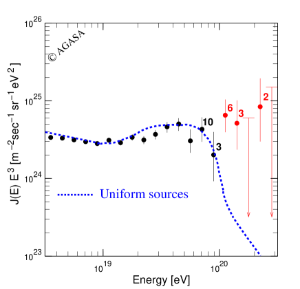
Figure 3: The flux of cosmic rays at high energies. The dashed line illustrates the GZK cut-off. (I thank Masahiro Takeda for permission to use this Figure.)

We now show how non-linear relativity modifies these thresholds. We present a modified argument proving that threshold anomalies do not depend on the complex issue of how to formulate energy and momentum conservation in non-linear relativity. For pedagogical reasons we take as an example gamma rays, for which one expects a cut-off due to interactions with the infra-red background. The cut-off energy corresponds to the kinematical condition for production of an electron-positron pair out of a gamma ray and an infra-red photon [163]. For a threshold reaction, the electron and positron have no momentum in the center of mass frame. Furthermore, in this frame the gamma ray and the infra-red photon have the same energy. (Undeformed) energy conservation then implies that both photons have an energy equal to the rest energy of an electron $m_{e}$. We can draw these conclusions since $m_{e}\ll E_{P}$, so that any corrections imposed by our theory are negligible.

We then need to perform a boost transformation from the center of mass frame to the cosmological frame. This can be pinned down by the condition that one of the photons be redshifted to the infra-red background energy. Since in this process all energies involved are again sub-Planckian we can use plain special relativistic formulae to conclude that $E_{IR}=(1-v)\gamma m_{e}$, and since $\gamma\gg 1$ (implying $1-v\approx 1/(2\gamma^{2})$) we have:

$$\gamma={m_{e}\over 2E_{IR}}$$ (55)

The same boost transformation blueshifts the other photon to our predicted value for the gamma ray threshold energy. This operation, however, has to be performed with the corrected non-linear boost. The uncorrected threshold energy is

$$E_{th0}=\gamma(1+v)m_{e}\approx 2\gamma m_{e}={m_{e}^{2}\over E_{IR}}$$ (56)

This now becomes:

$$E_{th}=U^{-1}(E_{th0})$$ (57)

since the non-linear boost derives from $U(E_{th})=\gamma(1+v)U(m_{e})$, and we have $U(m_{e})\approx m_{e}$. We thus arrive at (57) without using correction to (linear) energy conservation, using only one non-linear boost.

For UHECRs one considers the interaction of protons and CMB photons, and the threshold for pion production (e.g. [68]). An identical argument leads to the corrected threshold:

$$E_{th}=U^{-1}(E_{th0})=U^{-1}{\left({(m_{p}+m_{\pi})^{2}-m_{p}^{2}\over E_{CMB}}\right)}$$ (58)

where $m_{p}$ and $m_{\pi}$ are the proton and pion rest masses, and $E_{CMB}$ is the photon CMB energy in the cosmological frame. It was shown in [68] that it is possible to resolve the UHECR anomaly, while preserving an invariant energy scale of the order of the Planck energy. One may choose, for instance,

$$f_{1}={1\over(1+\lambda_{1}E)(1-\lambda E)}$$ (59)

with $\lambda_{1}^{-1}\approx 10^{11}Gev$ and $E_{P}=\lambda^{-1}$ (which may be of order $10^{19}$ Gev).

Another solution is to allow for a non-universal $U$ [214]. Different particles could then have a different $U$, or $U$ could depend on the rest mass $m$ of the particle on which it acts. One can then use the proton mass as an automatic extra scale in the problem, ensuring that the Planck scale is invariant and that the UHECRs threshold is raised.

A large number of variations around this theme have been put forward, e.g. [188, 79]. On a very different front, spontaneous symmetry breaking of Lorentz invariance [166] has also been used as a possible explanation for threshold anomalies.

Other implications of non-linear relativity for other areas of high energy astrophysics have been studied. Processes such as vacuum Cerenkov radiation ($e^{-}\rightarrow e^{-}\gamma$), photon decay $\gamma\rightarrow e^{+}e^{-}$, and other exotic processes are kinematically possible in some of these theories, leading to constraints upon their parameter space [196, 210]. Synchrotron emission from the Crab nebula was used in [215] to further tighten these constraints, but this work has been criticized for being model dependent (in the sense that it depends on more than kinematical arguments) [216, 217].

Finally the authors in [218] have used effective field theory to to find dimension 5 operators that do not mix with dimensions 3 and 4 and lead to cubic modifications of dispersion relations for scalars, fermions, and vector particles. Clock comparison experiments bound these operators at $10^{-5}/E_{P}$.

6.4 Theoretical developments

The outline of non-linear relativity given above leaves many questions unanswered, and considerable work is currently in progress.

Foremost, there is the problem of how to deal with composite systems. With the loss of linearity, the kinematic relations valid for single particles need not be true for composite systems. This is a desirable feature: non-linearity builds into the theory the concept of elementary particle, clearly differentiating between fundamental particles and composites.

The matter appears at first when defining a covariant law of addition of energy and momentum. The most straightforward definition (chosen in [207]) is

$$p_{a}^{(12)}=U^{-1}(U(p^{(1)}_{a})+U(p^{(2)}_{a}))$$ (60)

but it quickly leads to inconsistencies, e.g. it implies that a set of particles satisfying $E\ll E_{P}$ can never have a collective energy larger than $E_{p}$. This is blatantly in contradiction with observation. A possible solution is to note that the $U$ used for a system of, say, two particles need not be the same as that used for single particles, with $p_{a}^{(12)}=U^{-1}_{2}(U(p^{(1)}_{a})+U(p^{(2)}_{a}))$. A possible choice for a system of $n$ particles is then $U_{n}=U[p_{0};\lambda/n]$, that is a system of $n$ elementary particles should satisfy kinematical relations obtained from a map for which the Planck energy $E_{P}=\lambda^{-1}$ is replaced by $nE_{P}$.

Thus:

$$p^{(12)} \equiv p^{(1)}\oplus p^{(2)}$$ (61)

$$= U^{-1}\left[p_{0};\lambda/2\right]((U[p_{0};\lambda](p^{(1)})+U[p_{0};\lambda](p^{(2)}))$$

This defines a new, generally nonlinear, composition law for energy and momenta, which we denote by $\oplus$ to indicate that it is not ordinary addition. In general

$$p^{(1...n)}=U^{-1}[p_{0};\lambda/n](U[p_{0};\lambda](p_{1})+...+U[p_{0};\lambda](p_{n}))$$ (62)

With this definition a system of $n$ particles satisfies a system of transformations obtained from $U[p_{0};\lambda/n]$ via (43), equivalent to the usual ones but replacing $\lambda$ with $\lambda/n$. As a result, the collective momentum $P^{(N)}=p^{(1...n)}$ satisfies deformed dispersion relations with $\lambda$ replaced by $\lambda/n$. This can never lead to inconsistencies, because if all $n$ particles of a system have sub-Planckian energies then the total will still be sub-Planckian, in the sense that $E_{tot}\ll nE_{P}$. This addition law is generally commutative but non-associative, a feature expected of any addition law incorporating the concept of elementary particle.

There are other solutions to this problem. The embedding proposed in [199] amounts to a choice of $U_{2}$ which depends on the momentum of each individual particle according to a well defined formula.

Once addition rules are defined, the law of energy and momentum conservation is straightforward to implement; with the obvious exception of processes in which the number of particles changes. For an example of energy conservation in a process where different particles satisfy different dispersion relations see [117].

Another theoretical development concerns the position space picture of these theories (which are more usually constructed in momentum space). With loss of linearity, duals no longer mimic one another, that is, vectors no longer transform according to the inverse (linear) transformation of co-vectors. A number of solutions may be found, either involving [178] or avoiding non-commutative geometry [173]. The possible relation to quantum groups has long been known [174, 175, 197, 156, 209, 208, 60, 61, 156, 202, 203] (see also [185]).

It is obvious that one may recover linearity by embedding the theory into a higher number of dimensions. This approach is very elegant, and has been implemented in [199] (where an identification with deSitter space is accomplished) and in [200]. An alternative way to linearize the theory is to introduce a modified boost parameter [207, 170, 171].

A considerable amount of work has also gone into formulating field theory. Canonical quantization, and the set up of the Fock space have been examined [68, 189]. While scalar fields are straightforward to implement [68, 173], fermions are far more complicated [198, 205, 204]. Nonetheless, [186] showed how to produce non-linear realizations of the Poincaré group for arbitrary mass and spin. A supersymmetric extension of the Poincaré algebra was also studied.

Another field theory ramification resulted from the realization that neutrino flavour states do not satisfy standard dispersion relations and therefore transform according to a non-linear realization of the Lorentz group [117]. This has dramatic implications for the endpoint of $\beta$ decay; for instance one may accommodate a fit with $m_{\nu}^{2}<0$ (as suggested by experiment) without introducing acausal behaviour. In general it is found that $f_{1}^{2}$ does not need to be positive and so $m^{2}<0$ and tachyonic acausal behaviour cannot be identified. This feature was used to remove the tachyonic ground state of bosonic string theory in [77].

But perhaps the most tantalizing theoretical problem faced by this approach is how to do general relativity based on non-linear relativity [190, 78]. If one builds position space so that the space-time transformations are still linear (albeit energy dependent), a metric can still be defined, even though the metric tensor is now energy dependent [173]. In some sense, the metric “runs” with the energy, and general relativity can be set up in a straightforward fashion [78]. If, on the other hand, at high energy (or at small distances) the concept of metric simply disintegrates, the problem becomes potentially much more complicated.

7 “Black” holes and other compact objects

A major issue under investigation is the fate of black holes in the various VSL theories. This was first studied [75] in the context of the VSL theories presented in Section 3.4. The general aspect of the solutions is very similar to the solutions previously found by Brans and Dicke [10]:

$$ds^{2} = -F^{2\over\lambda}d\xi^{2}+{\left(1+{\rho_{0}\over\rho}\right)}^{4}F^{2(\lambda-C-1)\over\lambda}(d\rho^{2}+\rho^{2}d\Omega^{2})$$ (63)

$$c = c_{0}F^{C\over a\lambda}$$ (64)

with

$$F = {1-\rho_{0}/\rho\over 1+\rho_{0}/\rho}$$ (65)

$$\lambda^{2} = (C+1)^{2}-C(1-\kappa C/(2a^{2}))$$ (66)

(see [10] for an explanation of the coordinates used, and [75] for a relation between the various constants in this solution and the parameters of the theory). In a limiting case of the parameters of the theory, one may also recover the Schwarzschild solution, in which case $c$ varies in space according to:

$$c=c_{\infty}{\left(1-{2Gm\over c_{\infty}^{2}r}\right)}^{b-a\over 2\kappa}$$ (67)

We see that the speed of light either goes to zero or to infinity at the horizon (depending on the couplings’ signs). This property can be generally proved, and a simple condition for $c=0$ at the horizon was identified in [75].

This result suggests that the singularity at $r=0$ (and in some cases at the horizon) is physically inaccessible, not just in the sense that information cannot flow from it into the asymptotically flat region, but also in the sense that no observer starting from the asymptotically flat region can actually reach it. The singularity lies in a disconnected piece of the manifold, which should simply be excised as unphysical. It is tempting to conjecture that all singularities are subject to the same constraint, in which case VSL seems to have eliminated the singularity problem, by means of a stronger version of the cosmic censorship principle. A similar argument regarding the cosmological singularity in Brans-Dicke theories was put forward in [219]. However these remarks still belong to the realm of conjecture.

More generally, the removal of singularities in VSL may be related to the presence of a maximal acceleration [194, 195] in some of these theories. An interesting condensed matter analogy may be found in [220], where quantum liquids are used to simulate the behavior of the quantum vacuum in the presence of the event horizon. It is found that in most cases the quantum vacuum resists the formation of the horizon.

Since the speed of light vanishes at the Schwarzschild radius, it is not surprising that stellar collapse [75] and the properties of compact objects [221] are ultimately very different in these theories. The Oppenheimer-Snyder solution, in which a spherical dust ball collapses, was found in [75]. As the surface of the star approaches its Schwarzschild radius, all processes freeze-out. We are left with a Schwarzschild-sized remnant. Neutron stars were also extensively studied in [221]. For certain choices of parameters VSL neutron stars are much smaller than those in GR, and the dependence of their mass on the strength of the coupling between $\psi$ and matter is extremely strong. Thus the existence of neutron stars was used to place constraints on the theory’s parameters (even though the analysis is very sensitive to the equation of state used).

Black hole thermodynamics in VSL theories has also been studied under simplified assumptions, namely that the usual area formulae remain valid. Assuming a fixed black hole mass and the standard form of the Bekenstein-Hawking entropy, [136] have argued that the laws of black hole thermodynamics disfavor models in which the fundamental electric charge $e$ changes. Indeed if the black hole entropy is still given by

$$S={k_{b}\pi G\over\hbar c}{\left(M+{\sqrt{M^{2}+Q^{2}/G}}\right)}^{2}$$ (68)

and if $\hbar$, $G$ and $M$ remain constant, there is a clear difference between varying-$c$ and varying-$e$ theories. With similar assumptions, [222] then showed that severe constraints apply to VSL. This issue is related to the fate of the second law of thermodynamics as discussed in [132], and work in this area may be criticized along the same lines used above. Foremost, it is probable that particle production (and so Hawking radiation) would have to be radically modified (as suggested in [35]). A more complete study of this issue in dilaton theories may be found in [223]; see also [224] for a 2D stringy black hole.

For further work on black holes and varying constants see [225, 149]. It should be obvious that deformed dispersion relations (as those encoded by non-linear relativity) will translate into a non-thermal spectrum for the Hawking radiation. Some preliminary work on this topic may be found in [78, 211] (see also [212, 213]).

8 The observational status of VSL

In the middle of the current observational revolution in cosmology, it’s easy to forget that some nasty surprises have also fallen from the sky. Examples include claims for cosmic acceleration [1, 2, 3, 4], or the mounting evidence [19, 18] for a redshift dependence in the fine structure constant $\alpha$. Cosmologists can no longer, as in Dirac’s quote opening this paper, make “any assumptions that they fancy”; instead it appears that they must grapple with the issue of selecting which observations to take seriously. Most of what passes for observation in cosmology is plagued by systematic errors. Some of these “facts” could evaporate like fog should a new technological revolution come on line unexpectedly.

It is nonetheless interesting that several observational puzzles can be solved by VSL. With appropriate supplementary observations, the redshift dependence in $\alpha$ could be seen as the result of a varying $c$. Another puzzle, already studied in Section 6.3, was the observation of rare very high energy cosmic rays, in conflict with standard kinematic calculations based on special relativity, which predict a cut-off well below the observed energies. This could represent the first experimental mishap of special relativity, and evidence for some VSL theories. Finally, even the accelerating universe may be part of a varying $c$ picture of the world.

How can this meager evidence be extended? Unfortunately there are two obstacles to the observation of a varying speed of light. The first relates to the discussion in Section 2 and affects those aspects of VSL which are not dimensionless. It is easy to place oneself in a no-win situation (e.g. by defining units in which $c$ is a constant), but as explained in Section 2 the impasse may be solved by testing the dynamics of the theory. The issue of testability is more direct regarding the dimensionless aspects of a varying $c$.

More seriously, however, all tests of a varying $c$ face a second hurdle: the effects predicted are invariably either well beyond the reach of current technology, or at best on the threshold.

In what follows we describe a number of observations which would either provide positive detection of VSL effects, or imply constraints upon the parameters of the theory. We also stick the neck out, venturing a number of predictions of the theory.

8.1 Changing-$\alpha$ and varying-$c$

Figure 4: The data points are the QSO results for the changing $\alpha$. The solid line depict theoretical prediction in several varying-$\alpha$ models.

Perhaps the most extraordinary observation with relevance for VSL is the work of Webb et al [19] and Murphy et al [18] (hereafter referred to as the “Webb results” for historical reasons). These authors have reported evidence for a redshift dependence in the fine structure constant $\alpha=e^{2}/(\hbar c)$. This evidence was provided by a new observational many-multiplet technique, which exploits the extra sensitivity gained by studying relativistic transitions to different ground states, using absorption lines in quasar (QSO) spectra at medium redshift. The trend of these results is that the value of $\alpha$ was lower in the past, with $\Delta\alpha/\alpha=(-0.72\pm 0.18)\times 10^{-5}$ for $z\approx 0.5-3.5$. These results are displayed in Fig. 4. For non-“fundamentalists” (see Section 2.2 for a definition), the obvious question is: If $\alpha$ is varying, what else must be varying: $e$, $c$, $\hbar$, or a combination thereof? Could such a matter be resolved by experiment?

As explained in Section 2, such a matter can only be settled once a concrete theory is proposed, with a dynamics capable of selecting a preferred system of units. This dynamics may then be subjected to further experimental scrutiny. Unfortunately the actual $\alpha(z)$ observations are not capable of distinguishing between these theories. The dynamical equations for variations in $\alpha$ invariably take the form

$$\Box{\delta\alpha\over\alpha}=F(\rho)$$ (69)

In varying $e$ theories [25, 11, 26] one may have for instance:

$$F(\rho)=(2/\omega){\cal L}_{em}=(2/\omega)\zeta_{m}\rho_{m}$$ (70)

where $\zeta$ is the ratio between $E^{2}-B^{2}$ and $E^{2}+B^{2}$. In covariant VSL theories [35]) one has

$$F(\rho)=-(bq/\omega){\cal L}_{M}$$ (71)

and in VSL theories with hard breaking of Lorentz invariance one may have [72]

$$F(\rho)=-4\pi G\omega p(\rho).$$ (72)

In all these cases the wave (Box) operator in a homogeneous Universe is

$$\Box\psi=-\ddot{\psi}-3{\dot{a}\over a}\dot{\psi}$$ (73)

where $\psi\propto\delta\alpha/\alpha$, so the equations are formally identical, of the form

$$\ddot{\delta\alpha\over\alpha}+3{\dot{a}\over a}\dot{\delta\alpha\over\alpha}=-F(\rho)$$ (74)

and it is always possible to fit the Webb results with appropriate parameters.

Notice, however, that although all these theories reveal the same $\alpha(z)$, this depends upon the cosmological model, e.g. how much cosmological constant is present. In all these theories expansion acts as a friction force via the term in $\dot{a}/a$ in Eqn (74). Thus the current acceleration of the universe cannot be ignored and has a clear imprint upon the function $\alpha(z)$. Typically the onset of acceleration suppresses variations in whatever “varying” constant.

This is of crucial importance when attending to other constraints on varying alpha theories. Geonuclear tests, such as the Oklo natural nuclear reactor [226, 227] severely constrain variations in $\alpha$ at low redshift. Thanks to the cosmological constant varying alpha theories invariably accommodate low redshift constraints, while explaining the Webb results.

Given the non-discriminatory nature of $\alpha(z)$ we conclude that to distinguish between varying $e$ and varying $c$ theories one must look elsewhere. The status of the equivalence principle in these theories turns out to be a good solution. The varying $e$ theories [25, 11, 26] violate the weak equivalence principle, whereas VSL theories do not[40, 37]. The Eötvös parameter

$$\eta\equiv{\frac{2|a_{1}-a_{2}|}{a_{1}+a_{2}}}$$ (75)

is of the order $10^{-13}$ in varying $e$ theories, just an order of magnitude below existing experimental bounds. The STEP satellite could soon rule out the varying $e$ theories capable of explaining the Webb et al results [81].

For further varying alpha work in the context of brane world cosmology see [88]; an analytical supergravity model may be found in [228]. Also [40] is an example of a varying alpha model based on a VSL theory in which $c(t)$ is pre-given (see discussion in Section 3.1).

8.2 Supernovae results

Figure 5: The Hubble diagram built from Supernovae results (data points) suggests a Universe with 30% normal matter and 70% cosmological constant (plotted curve). However any other form of repulsive gravity could be made to fit the data.

Recent astronomical observations of distant supernovae light-curves have been realized by The Supernovae Cosmology Project and the High-z Supernova Search [1, 2, 3, 4]. These have extended the reach of the Hubble diagram to high redshifts and provided evidence that the expansion of the universe is accelerating (see Fig. 5).

A first question is how to interpret the Hubble diagram in VSL theories. Among other matters, the link between luminosity distance and look-back time is obviously modified: with a higher $c$ in the past objects with the same look-back time are further away [230, 231, 233, 72, 229]. If, however, one takes into account the fine-structure results of Section 8.1, one finds that any corrections to the construction of the Hubble diagram must be very small [72], unless very contrived variations in $e$, $G$ and $\hbar$ are introduced [232]. Therefore, even in VSL theories it looks as if the universe is accelerating.

This may imply that there exists a significant positive cosmological constant, $\Lambda$. If $\Lambda>0$, then cosmology faces a very serious fine tuning problem, and this has motivated extensive theoretical work. There is no theoretical motivation for a value of $\Lambda$ of currently observable magnitude; a value $10^{120}$ times smaller than the “natural” Planck scale of density.

One possible explanation is VSL [72]. In such theories the energy density in Lambda does not need to remain constant as in the standard theory, and thus does not require fine tuning. Indeed it is possible to set up theories in which the presence of Lambda drives changes in $c$, which in turn convert the vacuum energy into ordinary matter. In such theories the supernovae results can be explained without any need to fine-tune the initial conditions, in fact with all parameters of the theory being of order one [72].

In addition there is a strange, not often noted coincidence between the redshifts at which the Universe starts accelerating and those marking the onset of variations in $\alpha$. This coincidence can be explained within the framework of these VSL theories, for the reason cited above: acceleration acts as a brake on any constant variation. Thus in [72] both the Webb and supernovae results are fitted using the same set of parameters.

We should however point out that the supernovae results can be more modestly explained by quintessence, a replacement for the cosmological constant not dissimilar from the inflaton or dilaton fields [234].

8.3 Observations on the edge

There are other relevant detections of variations in supposed constants of nature, with obvious implications for VSL. However, we should stress that the uncertainties here are larger than in the results mentioned above. What follows merits interest but also caution.

Variations in other “fine structure constants” (such as the weak and strong $\alpha$) have not been neglected [235, 237]. In most VSL theories (e.g. [35]) all $\alpha$’s are bound to vary, since they must remain proportional to each other, given their form $\alpha_{i}=g^{2}/(\hbar c)$, where $i=em,W,S$ (electromagnetic, weak and strong). Variations in $\alpha_{W}$ from beta decay were examined in [168]. The Oklo natural reactor implies that the fermi constant $G_{F}$ could not have differed by more than 2% a few billion years ago. However, [168] claim to have found an apparent discrepancy between the current value of $G_{F}$ and that inferred from geochemical double-beta decay for 82Se; and also between results for old and young minerals of 82Se and 130Te. Although the Oklo constraints are themselves very model-dependent, these results don’t seem to fit well with each other or with any varying constant theory. They depend on a large number of geological assumptions.

A further claim for variation in a “constant” of nature was obtained from vibrational and rotational atomic lines originating in faraway systems. Naively one might think that such lines “measure” $\hbar$, but closer inspection reveals that they are sensitive to the dimensionless parameter $\mu=m_{p}/m_{e}$, the ratio between the proton and electron mass. A 3-sigma detection:

$${\Delta\mu\over\mu}=(5.02\pm 1.82)\times 10^{-5}$$ (76)

at a redshift of order 3 has been reported in [238]. Whether or not a 3-sigma result is to be declared a detection is of course debatable, but such a detection would have a strong bearing upon VSL theories.

Perhaps unsurprisingly, VSL theories have been proposed which impinge upon the issue of the dark matter in the universe [50, 44, 55, 62]. For instance, the bimetric theory presented in [50] contains a length scale of galactic size. For distances shorter than this scale, the theory reduces to General Relativity, but beyond this scale gravity becomes much stronger. The theory can explain the observed galactic rotation curves, doing away with the need for galactic dark matter. Likewise, the theory provides an explanation for the observed value of Hubble’s constant in relation to observed matter, without dark matter or energy.

In an orthogonal approach VSL may be used to produce dark matter candidates, such as in the theory proposed in [62] (as already mentioned in Section 3.3). Here double-branched deformed dispersion relations allow for high-momentum, low-energy particles to be left over from the Big Bang. However these double-valued dispersion relations appear to be forbidden by the criteria for non-linear Lorentz invariance spelled out in Section 6.2 (see also [68]).

The Pioneer anomaly is another result causing consternation [239]. Could gravity go so horribly wrong at distances smaller than 100 AU? The fact that most VSL (or varying-$e$) theories produce a fifth force [37] might lead one to think that VSL could explain the Pioneer anomaly. However, the predicted effect in VSL is invariably very small. The problem is to come up with a theory which fits Solar system data, while predicting significant novelties at $20-40$ AU. This rules out any $1/r^{2}$ type of force, and a successful theory should somehow incorporate the solar system scale (just as the theory in [50] incorporates the galactic scale). For the VSL fifth force [37] this can only be contrived by including an appropriate potential.

8.4 Constraints on space-time varying $c$

For every VSL theory it is important to explore the range of constraints arising from standard tests of relativity. This includes effects upon planetary orbits (eg. the precession of the perihelion of Mercury), upon light (eg. gravitational light bending, or the radar echo time-delay). These effects were studied, for instance, in the model described in Section 3.4, [35, 75]. Tight constraints upon the parameters of this theory were derived and then imposed upon further work. This is a prototype of work which should, and in most cases has been done for all VSL theories proposed to date.

In addition one may explore general “theory-free” constraints. As explained above, one can construct VSL models which not only solve the homogeneity problem, but also produce a scale-invariant spectrum of Gaussian fluctuations. In this sense there is consistency with WMAP observations. In all these models, as in inflation, the fluctuations are produced in the very early universe. Late-time variations in $c$ would, in addition, affect the way in which these primordial fluctuations are processed into the actual CMB ansisotropies. For instance, the ionization history of the universe would be changed [241, 240, 242], since a different value of $\alpha$ would affect the binding energy of hydrogen and the cross section for Thomson scattering. With simplifying assumptions one may then show how the Doppler peak positions would be modified, and thus constrain variations in $\alpha$ at $z\approx 1000$ to a few percent. As pointed out in [242] the existence of an early reionization epoch (as suggested by MAP) may lead to considerably tighter constraints very soon, as the “reionization bump” may be useful for the purpose of constraining (or detecting) variations in $\alpha$. Sensitivity to variations in $\alpha$ as small as 0.1 % should in principle be achieved.

Another set of constraints arises from possible violations of charge conservation in VSL and other varying $\alpha$ theories[122, 164]. These constraints are very model dependent (e.g. the equations in [122] are tied to one specific way of implementing electromagnetism in the theories in Section 3.1; cf. [35]). Even if one takes their particular implementation, one finds that many $c(t)$ functions bypass these constraints easily. But they are interesting nonetheless, in particular for their implications for baryogenesis [122]. Similar limits may be derived from possible seasonal variations in Solar neutrino experiments [165]. Correlating charge conservation constraints with violations of the equivalence principle has also been examined [236].

The tests above refer to theories predicting space-time variations in $c$. Theories where the speed of light is color dependent have quite a different observational status, which has already been discussed. It concerns threshold anomalies and gamma ray timing experiments (see [243] for an update on the latter). We have already pointed out that the two types of theories may be overlaid.

8.5 Sticking the neck out

Any physical theory should stick the neck out and make experimental predictions, and in this respect VSL has not been shy.

A very promising area is cold atom clocks [244]. The search for the perfect unit of time has led to the the quest for very stable oscillatory systems, leading to a gain, every ten years, of about one order of magnitude in timing accuracy. Cold atom clocks may be used as laboratory “table-top” probes for varying $\alpha$, with a current sensitivity of about $10^{-15}$ per year. For all varying alpha theories based on an equation of the form (74) one finds a similar prediction for the current yearly variation in alpha, once the Webb results are fitted. It is found (e.g. by following a numerical integration as described in [25]) that at present:

$${\dot{\alpha}\over\alpha}\approx 2.98\times 10^{-16}h\quad{\rm year}^{-1}$$ (77)

with $H_{0}=100h$ Km sec^-1 Mpc^-1, $\Omega_{\Lambda}=0.71$ and $\Omega_{m}=0.29$. For $h=0.7$ this gives a fractional variation in alpha of about $2\times 10^{-16}$ per year, which should soon be within the reach of technology. Such an observation would be an incredible vindication of the Webb results. On the other hand this effect would become a further annoyance for those concerned with the practicalities of defining the unit of time.

Note that although this prediction is more or less the same for all causal varying $\alpha$ theories, it does depend on cosmological parameters like $\Omega_{\Lambda}$, $H$, or $\Omega$. For instance the cosmological constant is essential is suppressing variations in $\alpha$ nowadays, as already explained above. Without Lambda the current rate of variation in $\alpha$ would be of the order $10^{-14}$ per year.

Spatial variations of $\alpha$ are likely to be significant [37] in any varying alpha theory. For any causal theory the dynamical equation for $\alpha$ will take form (69), that is the left hand side will be a wave operator. This operator leads to the general equation (74) in the context of time variations in an expanding universe. However, near a static configuration of source masses, the wave operator reduces to the spatial Laplacian, so that we obtain a general linearized equation of the form

$$\nabla^{2}{\delta\alpha\over\alpha}=F(\rho)$$ (78)

Relative variations in $\alpha$ near a star are therefore proportional to the local gravitational potential. The exact relation between the change in $\alpha$ with redshift and in space (near massive objects) is model dependent, but eq.(78) provides the framework for predictions. For instance, we have

$${\frac{\delta\alpha}{\alpha}}=-{\frac{\zeta_{s}}{\omega}}{\frac{M_{s}}{\pi r}}\approx 2\times 10^{-4}{\frac{\zeta_{s}}{\zeta_{m}}}{\frac{M_{s}}{\pi r}}$$ (79)

for a typical varying $e$ theory, but

$${\frac{\delta\alpha}{\alpha}}=-{\frac{bq}{\omega}}{\frac{M_{s}}{4\pi r}}\approx 2\times 10^{-4}{\frac{M_{s}}{\pi r}}\;.$$ (80)

for the VSL theory described in Section 3.4. Here $M_{s}$ is the mass of the compact object, $r$ is its radius, and $\zeta$ is the ratio between $E^{2}-B^{2}$ and $E^{2}+B^{2}$. When $\zeta_{m}$ (for the dark matter) and $\zeta_{s}$ (for, say, a star) have different signs, for a cosmologically increasing $\alpha$, varying $e$ theories predict that $\alpha$ should decrease on approach to a massive object. And indeed one must have $\zeta_{m}<0$ in order to fit the Webb results. In VSL, on the contrary, $\alpha$ increases near compact objects (with decreasing $c$ if $q<0$, and increasing $c$ if $q>0$). In VSL theories, near a black hole $\alpha$ could become much larger than 1, so that electromagnetism would become non-perturbative with dramatic consequences for particle physics near black holes. In varying-$e$ theories precisely the opposite happens: electromagnetism switches off.

These effects are in principle observable using similar spectroscopic techniques to those of Webb, but applied to lines formed on the surface of very massive objects near us (in the sense of $z\ll 1$). For that, we need an object with a radius sufficiently close to its Schwarzchild radius, such as an AGN, a pulsar or a white dwarf, for the effect to be non-negligible. Furthermore we need the “chemistry” of such an object to be sufficiently simple, so that line blending does not become problematic.

Generally (i.e. for any matter configurations) the larger the gravitational potential differences, the stronger the effect. Indeed, for static configurations, both $\Delta\alpha/\alpha$ and the gravitational potential satisfy Poisson equations, with source terms related by a multiplicative constant. Hence the local value of $\alpha$ should map the gravitational potential, and one would need to have big variations in the gravitational potential to observe corresponding spatial variations in $\alpha$.

Another area currently being studied are forces of inertia in frame-dependent VSL theories (a matter briefly discussed in Section 4.1). High precision gyroscopes could soon put these theories to the test.

9 Upcoming attractions

As the last section should have made clear, the future of VSL is in the hands of observers. In such circumstances theorists are bound to continue with their musings. Some of these may lead to further predictions and should be taken very seriously; others carry little more than entertainment value. We close with an impressionistic list of upcoming areas of theoretical research.

One area in which not much work has been done is the relation between VSL and quantum mechanics. Right from the start (e.g. [30]) it was obvious that a varying $c$ implied a varying $\hbar$. This connection has clear physical implications, for example particle creation [35, 121]. But there is more: it could be that some of the strange properties of quantum mechanics – such as its non-locality [245] – are the result of a form of “faster than light” communication. Indeed, a VSL solution to the problem of quantum entanglement has been proposed using the bimetric VSL theory [246]. Such a theory removes the tension between macroscopic classical and local gravity and non-local quantum mechanics. On a different front, it is also conceivable that the non-locality of quantum mechanics could be used as a solution to the homogeneity problem (and even more interestingly, the source of cosmic structure). In this sense, quantum mechanics may already be a VSL theory. However, a concrete theory based on this idea is still missing.

Part of the reason for this intellectual black hole is the paucity of work on VSL quantum cosmology. A possible excuse arises from the exotic fact that in some VSL theories there is no quantum epoch! In the model of [30], for instance, as we go back in time we find an increasing $t/t_{P}$ (where we recall $t_{P}$ is the Planck time). Hence the universe does not have a quantum origin, and one need not invoke quantum cosmology to set its initial conditions. Moreover, after a sufficient number of Big Bang cycles, the value of $\Lambda$ in fundamental units will grow to be of order 1. Thus, quantum cosmology is in the future, not the past.

Nevertheless this is not a generic feature of VSL models, and some implications for quantum cosmology have been considered [135, 133]. Specifically, in [135] the Wheeler-DeWitt equation under a varying $c$ was written down in the mini-superspace approximation. The quantum potential was obtained and the tunnelling probability examined in both the Vilenkin and the Hartle-Hawking approaches. Thus a description for the quantum birth of the Universe in VSL cosmologies was found. As J. W. Moffat had already pointed out [29] the “problem of time” in quantum cosmology does not exist in VSL theories.

Another area where plenty of work is expected in the near future, is the inclusion of gravity in the theories presented in Section 6. These theories are motivated by the need to introduce new invariant scales corresponding to the quanta of space and time. They are phenomenological descriptions of quantum gravity. Thus it is important that they can describe curved quantum space-time and not only its gravity-free counterpart. As explained in Section 6.4 the issue of gauging non-linear realizations of the Lorentz group depends crucially on how to define position space in these theories [173]. The work in [78] is based on the simplest construction, and indeed is the only approach to bear fruit so far.

However other approaches can and should be pursued. If one starts from a non-linear realization of the Lorentz group in real space, then the problem reduces to gauging non-linear representations, following the steps of Kibble [247], who showed that General Relativity is the gauge theory of the Poincaré group. Yet another approach results if position space is recovered by means of a non-commutative geometry [178]. Then the issue is how to introduce curvature into non-commutative structures. However it has been suggested [248] that such an undertaking is impossible. Whatever the case it would be good to have alternatives to [78], describing gravity in the contect of non-linear relativity.

These are some wide avenues where the field is active, but of course the future is unpredictable. Therefore we close with some random ideas.

Perhaps VSL could ensue from theories with two time dimensions, one of the form $c_{1}t_{1}$, the other $c_{2}t_{2}$. The time compactification dynamics would then produce a varying $c$, leading to another interesting realization of VSL.

It has been suggested that VSL may modify completely our perception of space travel [35, 167]. Indeed VSL cosmic strings [35] could act as a source for spatial variations in the speed of light, causing an increase in $c$ along the string, within a possibly macroscopic radius (the string core itself is always microscopic). Thus they create a tunnel within which light travels at much higher speeds. This could make it possible to travel extremely fast throughout the Universe without the annoyances of time dilation (which could be made negligible).

Regarding time (rather than space) travel, the implications of VSL for the concept of time machines have never been explored. However causality is usually built into VSL theories.

It has also been suggested that VSL has something to say about the probability and quality of life in the universe [43].

References

- [1] S. Perlmutter et al, Ap. J. 483, 565 (1997); S. Perlmutter et al (The Supernova Cosmology Project), Nature 391 51 (1998).
- [2] P.M. Garnavich et al 1998 Ap.J. Letters 493:L53-57.
- [3] B.P. Schmidt, Ap. J. 507 (1998) 46-63.
- [4] A.G.Riess et al 1998 Ap. J. 116:1009.
- [5] C.B. Netterfield et al., Astrophys.J. 571: 604-614, 2002.
- [6] C.L.Bennet et al, astro-ph/0302207.
- [7] K. Olive, astro-ph/9901231.
- [8] P. Dirac, Nature 139 (1937) 323.
- [9] V. Canuto et al, Phys. Rev. D 16 (1977) 1643.
- [10] C. Brans and R. Dicke, Phys.Rev. 124, 925 (1961).
- [11] J.D. Bekenstein, Phys. Rev. D 25, 1527 (1982); Phys.Rev.D66:123514,2002.
- [12] J. Barrow, New Scientist, 2196-21 July, pp 28, 1999.
- [13] W. Thomson and P.G. Tait, Natural Philosophy, 1, 403 (1874).
- [14] A.S. Eddington, Fundamental Theory, CUP, Cambridge, 1946.
- [15] G. Ellis, Nature, 42, 563, 2003.
- [16] M.J. Duff, hep-th/0208093.
- [17] M.J. Duff, L.B. Okun, G. Veneziano, JHEP 0203:023,2002.
- [18] M.T.Murphy et. al, MNRAS, 327, 1208 (2001) .
- [19] J.K. Webb, V.V. Flambaum, C.W. Churchill, M.J. Drinkwater & J.D. Barrow, Phys. Rev. Lett. 82, 884 (1999).
- [20] H. Poincaré, “The value of science”, pp215; Modern Library Paperback edition, New York, 2001.
- [21] A. Einstein, Ann. d. Phys. 35 (1911).
- [22] J.Stewart, Phys. Rev. 38, 2071 (1931).
- [23] H. Buc, J. Franklin Inst. 214, 197 (1932).
- [24] P. Wold, Phys. Rev D 47, 217 (1935).
- [25] H.B. Sandvik, J.D. Barrow, J.Magueijo, Phys. Rev. Lett. 88, 031302 (2002); J.D. Barrow, H.B. Sandvik, J. Magueijo, astro-ph/0109414.
- [26] K. Olive and M. Pospelov, hep-ph/0110377.
- [27] J. Uzan, Rev. Mod. Phys. 75, 403, 2003; hep-ph/0205340.
- [28] C. Martins, Phil. Trans. Roy. Soc. Lond. A360, 2681, 2002.
- [29] J. W. Moffat, Int. J. Mod. Phys. D 2, 351 (1993).
- [30] A. Albrecht and J. Magueijo, Phys. Rev. D 59, 043516 (1999).
- [31] J.D. Barrow, Phys. Rev. D 59, 043515 (1999).
- [32] J.D. Barrow and J. Magueijo. Phys. Lett. B 447, 246 (1999).
- [33] J.D. Barrow and J. Magueijo, Phys. Lett. B 443, 104 (1998).
- [34] J.D. Barrow and J. Magueijo, Class. Quant. Grav. 16, 1435, 1999.
- [35] J. Magueijo, Phys. Rev. D 62, 103521, (2000).
- [36] A. Peres, gr-qc 0210066; Phys. Rev. Lett. 19 (1967) 1293.
- [37] J. Magueijo, J.D. Barrow, H.B. Sandvik, Phys.Lett. B549, 284, 2002.
- [38] R. Brandenberger, J. Magueijo, Imaginative cosmology, ’Large Scale Structure Formation; proceedings of the Kish Island School 1999’, Kluwer, Dordrecht, Pro 2000; hep-ph/9912247.
- [39] G. Ellis and J. Uzan, gr-qc/0305099.
- [40] J. W. Moffat, astro-ph/0109350.
- [41] http://einstein.stanford.edu/STEP/
- [42] G. Amelino-Camelia; Int. J. Mod. Phys. D11, 1643, 2002.
- [43] J. Magueijo, “A truly evolving universe” in “Science and ultimate reality – celebrating John Wheeler’s vision”, CUP 2003.
- [44] B. Bassett et al, Phys.Rev.D62:103518,2000.
- [45] C. Misner, K. Thorne and J. Wheeler, Gravitation.
- [46] M. A. Clayton, J. W. Moffat, Phys.Lett. B460 (1999) 263-270.
- [47] S. Coleman and S. Glashow, Phys. Lett. B405, 249-252, 1997.
- [48] M. A. Clayton, J. W. Moffat, Phys. Lett. B506, 177-186, 2001.
- [49] I. Drummond, gr-qc/9908058.
- [50] I. Drummond, Phys. Rev. D63, 043503, 2001.
- [51] M. A. Clayton, J. W. Moffat, Int. J. Mod. Phys. D12, 697, 2003; astro-ph/0203164.
- [52] M. A. Clayton, J. W. Moffat, JCAP 06 (2003) 006; gr-qc/0304058.
- [53] M.A. Clayton and J.W. Moffat, Int. J. Mod. Phys. D11, 187, 2002.
- [54] M.A. Clayton and J.W. Moffat, Phys. Lett. B477, 269, 2000.
- [55] S. Liberati, et al, Nucl. Phys. Proc. Suppl. 88, 259 (2000).
- [56] G. Amelino-Camelia et al, Int.J.Mod.Phys. A12, 607-624, 1997; G. Amelino-Camelia et al, Nature 393:763-765, 1998.
- [57] J. Ellis et al, Astrophys.J.535, 139-151, 2000.
- [58] J. Ellis, N.E. Mavromatos and D. Nanopoulos, Phys. Rev. D63, 124025, 2001; ibidem astro-ph/0108295.
- [59] G. Amelino-Camelia, Int. J. Mod. Phys. D11, 35, 2002; gr-qc/0012051; G. Amelino-Camelia, Phys. Lett. B510, 255-263, 2001.
- [60] J. Kowalski-Glikman, Phys. Lett. A286, 391-394, 2001 (HEP-TH 0102098); N.R. Bruno, G. Amelino-Camelia, J. Kowalski-Glikman, Phys. Lett. B522, 133-138, 2001.
- [61] G. Amelino-Camelia and S. Majid, Int.J. Mod. Phys. A15:4301-4324, 2000.
- [62] L. Mersini, M. Bastero-Gil, P. Kanti, Phys. Rev. D64 (2001) 043508.
- [63] C. Burgess et al, JHEP 0203 (2002) 043.
- [64] S. Alexander and J. Magueijo, hep-th/0104093.
- [65] S. Alexander, R. Brandenberger and J. Magueijo, hep-th/0108190.
- [66] J. Magueijo and L. Pogosian, Phys. Rev. D67, 043518, 2003.
- [67] J. Magueijo and L. Smolin, Phys.Rev.Lett. 88 (190403) 2002.
- [68] J. Magueijo and L. Smolin, Phys.Rev.D67, 044017, 2003.
- [69] G. Amelino-Camelia and T. Piran, Phys.Rev. D64 (2001) 036005.
- [70] J. W. Moffat, hep-th/0208122.
- [71] T. Jacobson and Mattingly, Phys. Rev. D 64, 024028 (2001).
- [72] J. D. Barrow and J. Magueijo, Astrophys. J. Lett. 532, L87-90 (2000).
- [73] E. Kiritsis, JHEP 9910 (1999) 010, hep-th/9906206.
- [74] S. Alexander, JHEP 0011 (2000) 017, hep-th/9912037.
- [75] J. Magueijo, Phys. Rev. D63, 043502, 2001.
- [76] L. Smolin, hep-th/0303185.
- [77] J. Magueijo and L. Smolin, “String theory and deformed dispersion relations”, preprint.
- [78] J. Magueijo and L. Smolin, “Gravity’s rainbow”, gr-qc/0305055.
- [79] R. Lehnert, gr-qc/0304013.
- [80] S. N. Manida, gr-qc/9905046.
- [81] S. S. Stepanov, physics/9909009, astro-ph/9909311.
- [82] L. Randall and R. Sundrum, Phys Rev Lett 83, 3370, 1999.
- [83] L. Randall and R. Sundrum, Phys Rev Lett 83, 4690, 1999.
- [84] G. Kalbermann and H. Halevi, qr-qc/9810083; G. Kalbermann, Int Jour Mod Phys A15, 3197, 2000.
- [85] D. Chung and K. Freese, Phys. Rev. D 62, 063513, 2000.
- [86] H. Ishihara, Phys Rev Lett 86, 381, 2001.
- [87] C. Csaki, J. Erlich, C. Grojean, hep-th/0012143.
- [88] D. Youm, hep-th/0108237.
- [89] D. Youm, Mod.Phys.Lett.A17:175-184,2002
- [90] D. Youm, Phys.Rev.D65:025008,2002.
- [91] D. Youm, Phys.Rev.D64:085011,2001
- [92] D. Youm, Phys.Rev.D63:125011,2001
- [93] E. Gravanis, N. Mavromatos, hep-th/0108008.
- [94] S. Kalyana Rama, Phys.Lett. B519 (2001) 103-110.
- [95] A. Kehagias and E. Kiritsis, JHEP 11, 22 (1999).
- [96] C. Grojean, F. Quevedo, G. Tasinato, I. Zavala, JHEP 0108:005,2001
- [97] H. Snyder, Physcal Review 71 (1947) 38.
- [98] R. Jackiw, S.-Y. Pi, Phys. Rev. Lett. 88 (2002) 111603.
- [99] P. Castorina, A. Iorio, D. Zappal , hep-th 0212238.
- [100] N. Seiberg and E. Witten, JHEP 9909 (1999) 32.
- [101] J. Ellis, N.E. Mavromatos, D.V. Nanopoulos, hep-th/0105206
- [102] D. Steer and M. Parry, Int. J. Theor. Phys. 41, 2255-2286, 2002
- [103] G. Vones gr-qc/0105076
- [104] J. Niemeyer, Phys. Rev. D65, 083505, 2002.
- [105] J. W. Moffat, hep-th/0105017.
- [106] I. Drummond and S. Hathrell, Phys. Rev. D22, 343, 1980.
- [107] G. Shore, Nucl. Phys. B460, 379, 1996; Nucl.Phys. B605 (2001) 455-466.
- [108] P. Teyssandier, gr-qc/0303081.
- [109] M. Novello and S. D. Jorda, Mod. Phys. Lett. A4, 1809 (1989).
- [110] G. Shore, gr-qc/0304059.
- [111] K. Scharnhorst, Phys. Lett B 236, 354 (1990); G. Barton, Phys Lett B 237, 559 (1990).
- [112] H. Nielsen and M. Ninomiya, Nuc. Phys. B141, 153 (1978); H. Nielsen and I. Picek, Nucl. Phys. B 211, 269 (1983); S. Chada and H. Nielsen, Nucl. Phys. B 217, 125 (1983).
- [113] S. Coleman and S. Glashow, Phys. Rev. D59, 116008, 1999.
- [114] D. Colladay and V. Kostalecky, Phys. Lett. B 344, 259 (1995); Phys Rev D52, 6224 (1995); Phys Let B 511, 209 (2001); V. Kostalecki, Phys Rev Lett 80, 1818, (1998).
- [115] O. Bertolami, C.S Carvalho, Phys. Rev. D61, 103002, 2000; O. Bertolami, hep-ph/0301191.
- [116] O. Greenberg, Phys Rev Lett 89, 2002.
- [117] M. Blasone, P. Pires-Pacheco, J. Magueijo, hep-ph/0307205.
- [118] A. Guth, Phys.Rev. D23 347 (1981); A. Linde, Phys. Lett B108, 1220 (1982); A. Albrecht and P. Steinhardt, Phys.Rev.Lett. 48 1220 (1982); A. Linde, Phys. Lett B 129, 177 (1983).
- [119] J. Magueijo and K. Baskerville, astro-ph/9905393, published by CUP, 2000.
- [120] P. Avelino and C. Martins, Phys. Rev. D67, 027302, 2003.
- [121] T. Harko, M. Mak, Class. Quant. Grav. 16, 2741, 1999.
- [122] S. Landau, P. Sisterna, H. Vucetich, Phys.Rev. D63 (2001) 081303.
- [123] J.W. Moffat, Phys. Lett. B506, 193, 2001; hep-ph/0102088.
- [124] M. Szydowski and A. Krawiec, gr-qc/0212068.
- [125] M. Biesiada and M. Szydowski. Phys.Rev. D62 (2000) 043514.
- [126] S. Chakraborty, N. Chakraborty, U. Debnath, gr-qc/0305064.
- [127] L. Chimento, A. Jakubi, Int.J.Mod.Phys.D10: 107-113, 2001
- [128] P. Gopakumar, G.V. Vijayagovindan, Mod.Phys.Lett.A16: 957-962, 2001
- [129] J. Barrow, gr-qc/0211074.
- [130] P. Avelino and C. Martins, Phys. Lett. B 459, 468, 1999.
- [131] D. Youm, Phys.Rev.D66: 043506, 2002.
- [132] Luis P Chimento, Alejandro S Jakubi, D. Pavon, Phys.Lett. B508 (2001) 1-5
- [133] D. Coule, Mod. Phys. Lett. A14, 2437, 1999.
- [134] J. Barrow, H. Sandvik and J. Magueijo, Phys.Rev.D65:123501,2002.
- [135] T. Harko, H.Q. Lu, M.K. Mak, Europhys. Lett.49: 814-820, 2000.
- [136] P. Davies, T. Davis, C. Lineweaver, Nature 418, 602-603, 2002.
- [137] M. Livio, astro-ph/0301615.
- [138] J. Mather et al, Astrophys.J. 354, L37-L40, 1990.
- [139] A. Albrecht et al, Phys. Rev. Lett. 76, 1413-1416 (1996); J. Magueijo et al. Phys. Rev. Lett, 76, 2617 (1996); J. Magueijo et al, Phys. Rev. D 54, 3727 (1996).
- [140] J. Magueijo, Astrophys. J. Lett. 528 L57-L60 (2000).
- [141] E. Komatsu et al, astro-ph/0302223.
- [142] E. Harrison, Phys. Rev. D 1, 2726 (1970).
- [143] Y. Zeldovich, MNRAS, 160, 1 (1972).
- [144] A. Linde and V. Mukhanov, Phys. Rev. D56, 535,1997.
- [145] J. Peebles, astro-ph/9805194.
- [146] A. Lue, G. D. Starkman, T. Vachaspati, hep-th/0303137.
- [147] “Principles of Physical Cosmology”, P. J. E. Peebles, Princeton University Press, New Jersey 1993.
- [148] J. Khoury, B. Ovrut, P. Steinhardt, N. Turok, Phys. Rev. D64, 123522, 2001.
- [149] F. Cooperstock and V. Faraoni, hep-th/0302080.
- [150] J. Barrow and D. Mota, gr-qc/0212032.
- [151] P. Avelino and C. Martins, Phys. Rev. Lett.85, 1370-1373, 2000.
- [152] C. Rovelli, Living Rev. Rel. 1 (1998) 1.
- [153] S. Carlip, Rept. Prog. Phys. 64 (2001) 885.
- [154] J. Polchinski, hep-th/9611050.
- [155] S. Forste, hep-th/0110055.
- [156] J. Lukierski and A. Nowicki, Int. J. Mod. Phys.A18, 7-18, 2003, and references therein.
- [157] Gambini and J. Pullin, Phys. Rev. D59 (1999) 124021.
- [158] J. Alfaro et al, Phys. Rev. Lett. 84 (2000) 2318.
- [159] G. Adunas et al Phys.Lett. B485 (2000) 215.
- [160] C. Rovelli, S. Speziale, gr-qc/0205108
- [161] P. Biermann and G. Sigl, Lect.Notes Phys. 576 (2001) 1-26.
- [162] M. Takeda et al, Astrophys.J. 522 (1999) 225; Phys.Rev.Lett. 81 (1998) 1163-1166.
- [163] D. Finkbeiner, M. Davis and D. Schlegel, Astro. Ph. 544, 81 (2000).
- [164] H. Vucetich, astro-ph/0211457.
- [165] M Torres and Vucetich, astro-ph/0303588.
- [166] J. W. Moffat, hep-th/0211167.
- [167] B. Palmer, D. Marolf, Phys.Rev. D67 (2003) 044012
- [168] A. Barabash, nucl-ex/0210011; Czech.J.Phys.50:455-461,2000, Eur.Phys.J.A8:137-140,2000.
- [169] G. Amelino-Camelia, Nature, 418, 34-35, 2002.
- [170] G. Amelino-Camelia, gr-qc/0205125.
- [171] G. Amelino-Camelia, D. Benedetti, F. D’Andrea, hep-th/0201245.
- [172] N. Bruno, Phys.Lett. B547 (2002) 109-115.
- [173] D. Kimberly, J. Magueijo and J. Medeiros, gr-qc/0303067.
- [174] A. Blaut, M Daszkiewicz, J. Kowalski-Glikman, hep-th/0302157
- [175] P. Czerhoniak, hep-th/0302036.
- [176] K. Tezuka, hep-th/0302126.
- [177] S. Mignemi, hep-th/0302065.
- [178] M. Daszkiewick, K. Imilkowska and J. Kowalski-Gilkman, hep-th/0304027.
- [179] S. Mignemi, gr-qc/0304029
- [180] C. Heuson, gr-qc/0305015.
- [181] D.V. Ahluwalia, gr-qc/0212128.
- [182] M. Toller, hep-th/0301153; math-ph/0301014.
- [183] D. Grumiller, W. Kummer, D. Vassilevich, Ukrainian J. 48 (2003) 329-333; hep-th/0301061.
- [184] Clifford Will, Theory and experiment in gravitational physics, CUP, 1993.
- [185] M. Gogberashvili, hep-th/0212251.
- [186] A. Chakrabarti, hep-th/0211214.
- [187] P. Kosinski, P. Maslanka, hep-th/0211057.
- [188] M. Toller, hep-ph/0211094.
- [189] I. Dadic, L. Jonke, S. Meljanac, hep-th/0210264.
- [190] S. Mignemi, hep-th/0210213; hep-th/0208062.
- [191] L. Gonzalez-Mestres, hep-th/0210141.
- [192] L. Gonzalez-Mestres, hep-th/0208064.
- [193] L. Freidel, J. Kowalski-Glikman, L. Smolin, hep-th/0307085.
- [194] A. Feoli, Int. J. Mod. Phys. D12, 271-280, 2003.
- [195] S. Kalyana Rama, Mod. Phys. Lett. A18, 527, 2003.
- [196] T. Jacobson, S. Liberati, D. Mattingly, hep-ph/0209264.
- [197] J. Lukierski, A. Nowicki, Czech.J.Phys.52, 1261, 2002.
- [198] J. Alfaro, H. Morales-Tecotl, L. Urrutia, Phys.Rev.D66:124006,2002.
- [199] J. Kowalski-Glikman, Phys. Lett. B547, 291-296, 2002.
- [200] P. McCarthy and R. Schafir, gr-qc/0304079.
- [201] J. Rembielinski, K. Smolinski, hep-th/0207031.
- [202] A. Granik, hep-th/0207113.
- [203] A. Ballesteros, N. Rossano Bruno, F. Herranz, hep-th/0305033.
- [204] D.V. Ahluwalia, M. Kirchbach, gr-qc/0207004.
- [205] M. Arzano, G. Amelino-Camelia, gr-qc/0207003
- [206] M. Visser, gr-qc/0205093.
- [207] S. Judes, M. Visser, gr-qc/0205067.
- [208] J. Kowalski-Glikman, S. Nowak, Int.J.Mod.Phys.D12: 299-316, 2003 .
- [209] J. Kowalski-Glikman, S. Nowak, Phys.Lett.B539:126-132,2002
- [210] T. Konopka, S. Major, New J.Phys.4:57,2002.
- [211] R. Casadio, L. Mersini, hep-th/0208050
- [212] R. Casadio, Class. Quantum Grav. 19 (2002) 2453-2462.
- [213] R. Casadio, hep-ph/0304099.
- [214] G. Amelino-Camelia, astro-ph/0209232.
- [215] T. Jacobson, S. Liberati and D. Mattingly, astro-ph/0212190.
- [216] G. Amelino-Camelia, gr-qc/0212002.
- [217] T. Jacobson, S. Liberati and D. Mattingly, gr-qc/0303001.
- [218] R. Myers and M. Pospelov, hep-ph/0301124
- [219] I. Quiros, gr-qc/0001007; I. Quiros, R. Bonal, R. Cardena, Phys. Rev. D62, 044042, 2000; I. Quiros, Phys.Rev.D61, 124026, 2000.
- [220] G.E. Volovik, gr-qc/0301043.
- [221] A. Whinnett, gr-qc/0304023.
- [222] S. Carlip, Phys.Rev.D67:023507,2003
- [223] M. Fairbairn and M. H. Tytgat, JHEP 0302, 005 (2003); [arXiv:hep-th/0212105].
- [224] E. C. Vagenas, JHEP 0307:046, 2003; hep-th/0307192.
- [225] H. Shojaie, M. Farhoudi, astro-ph/0209453.
- [226] A. Shylakhter, Nature 264, 340 (1976).
- [227] Y. Fujii et al, Nucl. Phys. B, 573, 377 (2000); T.Damour and F.J. Dyson, Nucl. Phys. B, 480, 37 (1996)
- [228] V. Kostelecky, R. Lehnert and M. Perry, astro-ph/0212003.
- [229] J.W. Moffat, Int. J. Mod. Phys. D12, 281-298, 2003.
- [230] Ll. Bel,gr-qc/9809051, gr-qc/9905016, gr-qc/0306091.
- [231] E. Alvarez, Ll. Bel, Astrophys.J. 179, (1973) 39.
- [232] Ll. Bel, “Time dependence of and its concomitants”, preprint.
- [233] J. A. Belinchon, Gen.Rel.Grav. 32 (2000) 1487-1498.
- [234] C Wetterich, Nucl. Phys B. 302 668 (1988); B. Ratra and J. Peebles, Phys. Rev D37 (1988) 321; I. Zlatev, L. Wang, & P. Steinhardt, Phys. Rev. Lett. 82 896-899 (1999)
- [235] N. Chamoun, S. Landau, H. Vucetich, Phys.Lett. B504, 1, 2001.
- [236] S. Landau, P. Sisterna, H. Vucetich, gr-qc/0105025.
- [237] D. Kimberly and J. Magueijo, preprint.
- [238] A. Ivanchik et al, Astronomy Letter, 28, 423, 2002.
- [239] J. Anderson et al, Phys. Rev. Lett. 81, 2858, 1998.
- [240] S. Landau, D. Harari, M. Zaldarriaga, Phys. Rev. D 63, 083505 (2001).
- [241] P.P. Avelino, C. Martins, G. Rocha, astro-ph/0001292; Phys.Rev. D62 (2000) 123508.
- [242] C. Martins, A. Melchiorri, G. Rocha, R. Trotta, P. Avelino, P. Viana; astro-ph/0302295
- [243] J. Ellis et al, A&A, 402 409 (2003) [astro-ph/0210124].
- [244] Y. Sortais et al, Physica Scripta T95, 50-57, 2001.
- [245] A. Valentini, quant-ph/0112151, NonLocality and Modality. Edited by T. Placek and J. Butterfield, Kluwer, 2002. pp. 81-103.
- [246] J.W. Moffat, quant-ph/0302061.
- [247] T. Kibble, J. Math. Phys. 2, 212-221, 1961.
- [248] E. Hawkins, math.QA/0211203.