KANAZAWA-22-05

November, 2022

Subcritical regime of hybrid inflation
with modular $A_{4}$ symmetry

Yoshihiro Gunji,(a) Koji Ishiwata,(a) Takahiro Yoshida${}^{\it(b),\,(c)}$

(a)Institute for Theoretical Physics, Kanazawa University, Kanazawa 920-1192, Japan

(b)Department of Information, Kaishi Professional University, Niigata 950-0916, Japan

(c)Department of Physics, Niigata University, Niigata 950-2181, Japan

1 Introduction

Inflation, a hypothesis of accelerated expansion of the Universe, is supported by the observation of the cosmic microwave background (CMB) radiation. It is driven by the vacuum energy at the early state of the Universe and it is realized by a slowly-rolling scalar field, called inflaton. According to decades of the observations and analysis of the CMB, some properties of inflation have been revealed. The latest results by Planck collaboration [1] report that the amplitude $A_{s}$ and spectral index $n_{s}$ of the scalar perturbation and the ratio $r$ of the tensor mode to the scalar mode are given by $A_{s}=(2.0989\pm 0.029)\times 10^{-9}~{}~{}(68\%\,{\rm CL})$, $n_{s}=0.9649\pm 0.0042~{}~{}(68\%\,{\rm CL})$, and $r<0.056~{}~{}(95\%\,{\rm CL})$. The results already exclude some of inflation models and future experiments are expected to measure the observables with more precision.

Besides the accelerated expansion of the Universe, the inflaton field plays another important role, i.e., reheating to create the radiation dominated Universe. Then the production of dark matter and baryons follows. Thus, it is tempting to consider an inflation model that provide the sequence of the thermal history after inflation. Moreover, the model would be motivated if it is controlled by an underlying symmetry. The modular symmetry and supersymmetry are the promising candidates.

The modular symmetry is the discrete symmetry associated with the compactification of the extra dimensions inspired by superstring theory. It has recently caught attention from the phenomenological point of view since Ref. [2] pointed out that it gives a consistent pattern of the neutrino mixing data [3, 4, 5, 6, 7, 8]. Variety types of symmetries have been studied so far; for instance, the modular $S_{3}$ [9], $A_{4}$ [2, 10, 11, 12, 13, 14, 15, 16, 17, 18, 19, 20, 21, 22, 23, 24, 25, 26, 27, 28, 29, 30, 31, 32, 33, 34, 35, 36, 37, 38, 39, 40, 41, 42, 43, 44, 45, 46, 47, 48, 49, 50, 51, 52], $A_{5}$ [53, 54, 55], and other modular groups [56, 57, 58, 59]. Quark masses and mixings are investigated in Refs.  [60, 61, 62, 63]. In the modular symmetric framework, soft supersymmetry breaking terms [64] and modular stabilization [65, 66, 67, 68, 69] are also discussed. For other phenomenological applications, for example, the application of modular symmetry to grand-unified theories is discussed in Refs. [70, 71, 72, 73, 74, 75, 76, 77, 78]. Moreover, in cosmology, models with dark matter candidates [79, 80, 81, 82, 83, 84, 85, 86] have been considered and Refs. [87, 88, 89, 90, 91, 92, 93, 94, 95] have applied it to leptogenesis.

In the present study we apply the modular $A_{4}$ symmetry to inflation. Introducing three right-handed (s)neutrinos, we consider one of right-handed sneutrinos plays the role of the inflaton field. Since the typical model of the right-handed sneutrino inflation tends to be chaotic inflation due to the quadratic term, which is already excluded by the CMB observations, we extend the model to the $D$-term hybrid inflation by introducing a new Yukawa term. These days variety of new $D$-term hybrid inflation models have been proposed, depending on the symmetry of the Kähler potential; $R^{2}$ Starobinsky model [96, 97] appears from the superconformal symmetry [98], the chaotic regime emerges from the shift symmetry [99, 100], and $\alpha$-attractor [101] comes from their combination, which is called superconformal subcritical hybrid inflation [102]. A generalized version of the inflation model proposed in Ref. [102] is intensitively analyzed in Ref. [103]. In our paper we study the neutrino mixing and the dynamics of inflation based on the model in Ref. [103]. In the framework, an unconventional neutrino mixing pattern and the CP phases are obtained. We find that only the inverted hierarchy is consistent with the data and in the valid parameters the upper limit for the scale of the Majorana mass is obtained for successful inflation.

This paper is organized as follows. In Sec. 2, we introduce the supergravity model to study. Then neutrino masses and mixing pattern are discussed in Sec. 3. Here we show the predicted CP phases and the effective neutrino mass for the neutrinoless double beta decay. In Sec. 4, the dynamics of inflation is studied both analytically and numerically, especially focusing on the impact of the Majorana mass terms. Sec. 5 contains our conclusion.

2 The model

2.1 Brief review of modular symmetry

The modular symmetry is the geometric symmetry of the two dimensional torus. The two dimensional torus $T^{2}$ is defined by $\mathbb{C}/\Lambda$, i.e., the complex plane $\mathbb{C}$ divided by the two dimensional lattice $\Lambda=\{\sum_{i=1}^{2}n_{i}\omega_{i}\,|\,n_{i}\in\mathbb{Z}\}$ with basis vectors $\omega_{i}\in\mathbb{C}$. Here, the basis vectors are given by $\omega_{1}=2\pi R$ and $\omega_{2}=2\pi R\tau$ with $R\in\mathbb{R}$, and $\tau=\omega_{2}/\omega_{1}$ is the modulus defined in the upper half plane $\mathcal{H}=\{\tau\in\mathbb{C}\,|\,\mathrm{Im}\tau>0\}$. The same lattice is constructed using the basis vectors transformed as

$\displaystyle\begin{pmatrix}\omega_{2}^{\prime}\\ \omega_{1}^{\prime}\end{pmatrix}$ $\displaystyle=\gamma\begin{pmatrix}\omega_{2}\\ \omega_{1}\end{pmatrix}\,,\qquad\gamma\in SL(2,\mathbb{Z})\,,$ (2.1)

where

$\displaystyle\Gamma\equiv SL(2,\mathbb{Z})\equiv\biggl{\{}\gamma=\begin{pmatrix}a&b\\ c&d\end{pmatrix}\,\biggl{|}\biggr{.}\,\,a,b,c,d\in\mathbb{Z},\ ad-bc=1\biggr{\}}\,.$ (2.2)

Then, the modulus is transformed as

$\displaystyle\tau\to\gamma\tau=\frac{a\tau+b}{c\tau+d}\,.$ (2.3)

Eq. (2.3) is called modular transformation. It is seen that the transformation law of $\tau$ is the same for $\gamma$ and $-\gamma$. Then, the group of modular transformation is isomorphic to $PSL(2,\mathbb{Z})\equiv SL(2,\mathbb{Z})/\pm\mathbb{I}\equiv\bar{\Gamma}$, which is called modular group. The modular group is generated by two generators,

$\displaystyle S$ $\displaystyle=\begin{pmatrix}0&1\\ -1&0\end{pmatrix},\quad T=\begin{pmatrix}1&1\\ 0&1\end{pmatrix}\,,$ (2.4)

satisfying

$\displaystyle(ST)^{3}=S^{2}=\mathbb{I}\,.$ (2.5)

The modulus $\tau$ is transformed by $S$ and $T$ as

$\displaystyle\begin{split}S&:\,\tau\to-1/\tau\,,\\ T&:\,\tau\to\tau+1\,.\end{split}$ (2.6)

For a positive integer $N$, the principal congruence subgroup of level $N$ is defined by

$\displaystyle\Gamma(N)$ $\displaystyle=\biggl{\{}\begin{pmatrix}a&b\\ c&d\end{pmatrix}\in\Gamma\ \biggl{|}\biggr{.}\,\begin{pmatrix}a&b\\ c&d\end{pmatrix}\equiv\begin{pmatrix}1&0\\ 0&1\end{pmatrix}\,(\mathrm{mod}\,N)\biggr{\}}\,.$ (2.7)

Note that $\Gamma(1)=\Gamma$ and $-\mathbb{I}\not\in\Gamma(N)$ for $N>2$. Then, we introduce the groups $\bar{\Gamma}(N)$ as $\bar{\Gamma}(2)=\Gamma(2)/\pm\mathbb{I}$ and $\bar{\Gamma}(N)=\Gamma(N)\,(N>2)$. The quotient groups $\Gamma_{N}\equiv\bar{\Gamma}/\bar{\Gamma}(N)$ are called finite modular groups and the generators of $\Gamma_{N}$ have the additional relation,

$\displaystyle T^{N}=\mathbb{I}\,.$ (2.8)

It is known that the finite modular groups for $N=2,3,4,5$ are isomorphic to the non-Abelian discrete groups, $\Gamma_{2}\simeq S_{3}$, $\Gamma_{3}\simeq A_{4}$, $\Gamma_{4}\simeq S_{4}$, $\Gamma_{5}\simeq A_{5}$, respectively[104]. Under the modular transformation, the holomorphic functions of $\tau$, called the modular forms are transformed as

$\displaystyle f(\tau)$ $\displaystyle\to f(\gamma\tau)=(c\tau+d)^{k}\rho(\gamma)f(\tau)\,.$ (2.9)

Here $\rho(\gamma)$ is a unitary transformation of $\Gamma_{N}$ $(N>2)$ and $k$ is non-negative even integer, called modular weight.

In this study, we focus on $\Gamma_{3}$, i.e., $A_{4}$. Then, the modular forms $Y=(Y_{1},Y_{2},Y_{3})^{T}$ with representation of $A_{4}$ triplet and modular weight $2$ are given by [2]

$\displaystyle Y_{1}$ $\displaystyle=\frac{i}{2\pi}\biggl{[}\frac{\eta^{\prime}(\tau/3)}{\eta(\tau/3)}+\frac{\eta^{\prime}((\tau+1)/3)}{\eta((\tau+1)/3)}+\frac{\eta^{\prime}((\tau+2)/3)}{\eta((\tau+2)/3)}-\frac{27\eta^{\prime}(3\tau)}{\eta(3\tau)}\biggr{]}\,,$
$\displaystyle Y_{2}$ $\displaystyle=\frac{-i}{\pi}\biggl{[}\frac{\eta^{\prime}(\tau/3)}{\eta(\tau/3)}+\omega^{2}\frac{\eta^{\prime}((\tau+1)/3)}{\eta((\tau+1)/3)}+\omega\frac{\eta^{\prime}((\tau+2)/3)}{\eta((\tau+2)/3)}\biggr{]}\,,$ (2.10)
$\displaystyle Y_{3}$ $\displaystyle=\frac{-i}{\pi}\biggl{[}\frac{\eta^{\prime}(\tau/3)}{\eta(\tau/3)}+\omega\frac{\eta^{\prime}((\tau+1)/3)}{\eta((\tau+1)/3)}+\omega^{2}\frac{\eta^{\prime}((\tau+2)/3)}{\eta((\tau+2)/3)}\biggr{]}\,,$

where $\omega=e^{2\pi i/3}$ and $\eta(\tau)$ is the Dedekind eta-function defined by

$\displaystyle\eta(\tau)$ $\displaystyle=q^{1/24}\prod_{i=1}^{\infty}(1-q^{n}),\quad q=e^{2\pi i\tau}\,.$ (2.11)

The modular forms $Y_{i}\,(i=1\text{--}3)$ satisfy the relation,

$\displaystyle Y_{2}^{2}+2Y_{1}Y_{3}=0\,.$ (2.12)

They are transformed under $T$ and $S$ transformations as

$\displaystyle\begin{split}S&:\,Y(-1/\tau)=\tau^{2}\rho(S)Y\,,\\ T&:\,Y(\tau+1)=\rho(T)Y\,,\end{split}$ (2.13)

where

$\displaystyle\rho(S)$ $\displaystyle=\frac{1}{3}\begin{pmatrix}-1&2&2\\ 2&-1&2\\ 2&2&-1\end{pmatrix}\,,\quad\rho(T)=\begin{pmatrix}1&&\\ &\omega&\\ &&\omega^{2}\end{pmatrix}\,.$ (2.14)

It is assumed that the superfields, denoted as $Z^{I}$, are also transformed under $A_{4}$ as

$\displaystyle Z^{I}\to(c\tau+d)^{-k_{I}}\rho^{(I)}(\gamma)Z^{I}\,,$ (2.15)

where the modular weight $k_{I}$ will be determined later.

2.2 The superpotential and Kähler potential

$L$ $E^{c}=(e^{c},\,\mu^{c},\,\tau^{c})$ $N^{c}$ $H_{u}$ $H_{d}$ $S_{\pm}$
U(1) 00 00 00 00 00 $\pm q$
$A_{4}$ $\boldsymbol{3}$ $(\boldsymbol{1},\,\boldsymbol{1}^{\prime\prime},\,\boldsymbol{1}^{\prime})$ $\boldsymbol{3}$ $\boldsymbol{1}$ $\boldsymbol{1}$ $\boldsymbol{1}$
weight $-k_{L}$ $(-k_{e^{c}},-k_{\mu^{c}},-k_{\tau^{c}})$ $-k_{N^{c}}$ $-k_{H_{u}}$ $-k_{H_{d}}$ $-k_{S_{\pm}}$
Table 1: Field contents and their representations and modular weights.

We consider a supergravity model of inflation inspired by modular $A_{4}$ symmetry. In addition to the fields in the minimal supersymmetric standard model (MSSM), we introduce three right-handed neutrinos $N^{c}_{i}\,\,(i=1\text{--}3)$ and two new fields $S_{\pm}$. Here $S_{\pm}$ are gauge singlets under the MSSM gauge but are charged under a local U(1) with charge $\pm q\,(q>0)$. They play important roles during inflation.

The superpotential allowed under $A_{4}$ symmetry is given by

$\displaystyle W$ $\displaystyle\supset W_{E}+W_{N}+W_{\rm hyb}\,,$ (2.16)

where

$\displaystyle W_{E}$ $\displaystyle=\alpha_{1}e^{c}H_{d}(LY)_{\boldsymbol{1}}+\alpha_{2}\mu^{c}H_{d}(LY)_{\boldsymbol{1}^{\prime}}+\alpha_{3}\tau^{c}H_{d}(LY)_{\boldsymbol{1}^{\prime\prime}}\,,$ (2.17)
$\displaystyle W_{N}$ $\displaystyle=g_{1}(N^{c}H_{u}(LY)_{\boldsymbol{3}\mathrm{s}})_{\boldsymbol{1}}+g_{2}(N^{c}H_{u}(LY)_{\boldsymbol{3}\mathrm{a}})_{\boldsymbol{1}}\,,$ (2.18)
$\displaystyle W_{\rm hyb}$ $\displaystyle=\lambda S_{+}S_{-}(N^{c}Y)_{\boldsymbol{1}}+\Lambda(N^{c}N^{c}Y)_{\boldsymbol{1}}\,.$ (2.19)

The superpotential is similar to one considered in Ref. [105], but it is extended to accommodate the modular $A_{4}$ symmetry. The contents of the fields are listed in Table 1. The representation and the modular weights of the fields are also shown in the table, which is based on the model considered in Ref. [2, 11]; the right-handed neutrinos and the left-handed lepton doublets $L_{i}=(\nu_{Li},l_{Li})^{T}\,\,(i=e,\mu,\tau)$ are the $A_{4}$ triplets and the others are the singlets. Here the three different singlet representations $(\mathbf{1},\mathbf{1^{\prime\prime}},\mathbf{1^{\prime}})$ are assigned to the right-handed charged leptons $E^{c}=(e^{c},\mu^{c},\tau^{c})$, respectively. We will discuss the assignment of the modular weights soon later. In the superpotential, $\alpha_{i}\,\,(i=1\text{--}3)$, $g_{i}\,\,(i=1,2)$, and $\lambda$ are Yukawa coupling constants, and $\Lambda$ determines the mass scale of the right-handed neutrinos. By redefinition of the fields, the parameters $\alpha_{i}$, $\lambda$, $\Lambda$, and $g_{1}$ can be taken to be real without the loss of generality.

For Kähler potential, we adopt a class of the canonical superconformal supergravity model [106]. This type of model can be extended to the model with a parameter $\alpha$, which corresponds to the parameter of the superconformal $\alpha$ attractor model [101]. Recently the dynamics of inflation has been analyzed in a generalized version of the model [103]. In order to consider the similar inflation model, we consider the Kähler potential based on Ref. [103]:#1#1#1We adopt the Planck unit, where $M_{\mathrm{pl}}=1$ for the Planck mass $M_{\mathrm{pl}}$.

$\displaystyle K$ $\displaystyle=-3\log\Bigl(-\frac{\mathcal{N}}{3}\Bigr{missing})\,,$ (2.20)

where

$\displaystyle\mathcal{N}$ $\displaystyle=-|Z^{0}|^{n}\Bigl{(}-\frac{\Phi}{3}\Bigr{)}^{\alpha}\,,\quad-\frac{\Phi}{3}=1-\sum_{I}\frac{|Z^{I}|^{2}}{|Z^{0}|^{k_{I}}}\,.$ (2.21)

Here we have introduced a positive parameter $n$ in order to discuss the modular weights of the field generically. We take $Z^{0}$ as $Z^{0}=\bar{Z^{0}}=2\,\mathrm{Im}\,\tau$, In general, $\Phi$ includes additional terms, such as $(YN^{c}N^{c})_{\mathbf{1}}$ or $(\bar{Y}\bar{L}YL)_{\mathbf{1}}$ [2, 19]. In the current study we ignore them to focus on the simple setting.#2#2#2This is also motivated by the results given by Ref. [103]. In the literature it is shown such a simple Käher potential gives a consistent result with the CMB observations.

The Kähler potential is further divided into the modular and matter parts as $K=K^{\tau}+K^{\mathrm{m}}$, where

$\displaystyle K^{\tau}$ $\displaystyle=-3n\log(2\,\mathrm{Im}\,\tau)\,,\quad K^{\mathrm{m}}=-3\alpha\log\Bigl(-\frac{\Phi}{3}\Bigr{missing})\,.$ (2.22)

The matter part is constructed to be modular invariant. Then, under the modular transformation (2.3), the Kähler potential is transformed as

$\displaystyle K$ $\displaystyle\to K+3n\bigl{[}\log(c\tau+d)+\log(c\bar{\tau}+d)\bigr{]}\,.$ (2.23)

In the supergravity the combination of the Kähler potential and superpotential, which is defined by

$\displaystyle\mathcal{G}$ $\displaystyle=K+\log{W}+\log{\overline{W}}\,,$ (2.24)

should be modular invariant. Due to the invariance, the transformation of the superpotential is determined as,

$\displaystyle\begin{split}W&\to e^{i\alpha(\gamma)}(c\tau+d)^{-3n}W\,,\\ \overline{W}&\to e^{-i\alpha(\gamma)}(c\bar{\tau}+d)^{-3n}\overline{W}\,.\end{split}$ (2.25)

Namely, its modular weight is $-3n$. Consequently, the weight of fields should satisfy

$\displaystyle\begin{split}3n&=k_{H_{u}}+k_{H_{d}}=k_{S_{+}}+k_{S_{-}}+k_{N^{c}}-2=2k_{N^{c}}-2\\ &=k_{N^{c}}+k_{L}+k_{H_{u}}-2=k_{E^{c}}+k_{L}+k_{H_{d}}-2\,,\end{split}$ (2.26)

where $k_{e^{c}}=k_{\mu^{c}}=k_{\tau^{c}}=k_{E^{c}}$. Those are the generic conditions for the modular weights in the present model. For instance, if we further impose the following conditions:

$\displaystyle k_{H_{u}}=k_{H_{d}}\equiv k_{H}\,,\quad k_{S_{+}}=k_{S_{-}}\equiv k_{S}\,,$ (2.27)

the modular weights are uniquely determined for a given $n$ as

$\displaystyle k_{L}=1\,,\quad k_{N^{c}}=k_{E^{c}}=2k_{S}=k_{H}+1=(3n+2)/2\,.$ (2.28)

The value of $n$ is a free parameter and it may restrict possible terms in the Kähler potential. However, we do not consider this direction seriously in the current study.

After the modulus parameter $\tau$ is fixed, we redefine the chiral superfields as

$\displaystyle Z^{I}\to\check{Z}^{I}=Z^{I}\sqrt{3/|Z^{0}|^{k_{I}}}\,.$ (2.29)

Accordingly it is convenient to reparametrize the Yukawa couplings ($\alpha_{i}$, $g_{i}$, $\lambda$) and $\Lambda$ as ($\check{\alpha}_{i}$, $\check{g}_{i}$, $\check{\lambda}$) and $\check{\Lambda}$ to give rise to the same form of $W_{E}+W_{N}+W_{\rm hyb}$. Hereafter, we will write the model in this field basis and omit the ‘check’ symbol for a simple notation unless otherwise noticed. Namely, we use the superpotential given in Eqs. (2.17) – (2.19) and the Kähler potential $K^{\rm m}$ of the matter part with the function $\Phi$

$\displaystyle-\frac{\Phi}{3}=1-\frac{1}{3}\sum_{I}|Z^{I}|^{2}\,.$ (2.30)

For later calculation, we rewrite $W_{\rm hyb}$ as

$\displaystyle W_{\rm hyb}=\lambda_{i}S_{+}S_{-}N^{c}_{i}+\frac{1}{2}M_{ij}N^{c}_{i}N^{c}_{j}\,,$ (2.31)

where $(\lambda_{1},\lambda_{2},\lambda_{3})=\lambda(Y_{1},Y_{3},Y_{2})$ and

$\displaystyle M$ $\displaystyle=\Lambda\begin{pmatrix}2Y_{1}&-Y_{3}&-Y_{2}\\ -Y_{3}&2Y_{2}&-Y_{1}\\ -Y_{2}&-Y_{1}&2Y_{3}\end{pmatrix}\,.$ (2.32)

3 Neutrino masses and mixing pattern

In this section, we discuss the lepton sector, especially focusing on the neutrino mixing pattern. From the superpotential, the light neutrinos acquire masses in the seesaw mechanism [107, 108, 109, 110, 111, 112]. In our model, however, $S_{+}$ obtains a vacuum expectation value (VEV), denoted as $\langle S_{+}\rangle$, at the global minimum, which leads to an unconventional mass matrix for the light neutrinos [105]. In addition, the components of the mass matrices are given in a limited number of parameters due to $A_{4}$ symmetry, which results in the characteristic pattern of the neutrino mixing and CP phases in the lepton sector.

3.1 Neutrino masses and PMNS matrices

To give the mass matrices of the leptons, it is convenient to adopt canonically normalized field basis. The canonically normalized field $\hat{Z}^{I}$ is obtained by

$\displaystyle\hat{Z}^{I}=\sqrt{\alpha}Z^{I}\,.$ (3.1)

Here we have used $-\Phi/3\simeq 1$ at the global minimum. The validity of the approximation is guaranteed by $\expectationvalue{S_{+}}\ll 1$, which will be shown in Sec. 4. Accordingly we absorb the factor $\sqrt{\alpha}$ by introducing

$\displaystyle(\hat{\alpha}_{i},\hat{g}_{i},\hat{\lambda})=\alpha^{-3/2}(\alpha_{i},g_{i},\lambda)\,,~{}~{}~{}\hat{\Lambda}=\alpha^{-1}\Lambda\,,$ (3.2)

to give the same form of the superpotential.

Let us see the neutrino mass matrix. We rewrite Eq. (2.19) as

$\displaystyle W_{\rm hyb}=\hat{\lambda}_{i}\hat{S}_{+}\hat{S}_{-}\hat{N}^{c}_{i}+\frac{1}{2}\hat{M}_{ij}\hat{N}^{c}_{i}\hat{N}^{c}_{j}\,.$ (3.3)

where $(\hat{\lambda}_{1},\hat{\lambda}_{2},\hat{\lambda}_{3})=\hat{\lambda}(Y_{1},Y_{3},Y_{2})$ and

$\displaystyle\hat{M}$ $\displaystyle=\hat{\Lambda}\begin{pmatrix}2Y_{1}&-Y_{3}&-Y_{2}\\ -Y_{3}&2Y_{2}&-Y_{1}\\ -Y_{2}&-Y_{1}&2Y_{3}\end{pmatrix}\,.$ (3.4)

Then, the mass matrix of the neutrinos in the basis of $(N^{c}_{1},N^{c}_{2},N^{c}_{3},\tilde{S}_{-},\nu_{Le},\nu_{L\mu},\nu_{L\tau})$#3#3#3We use the same notation for the fermionic part as the chiral superfield for $N^{c}_{i}$ and the leptons in the MSSM while $\tilde{S}_{-}$ is the fermionic part of $S_{-}$. is given by

$\displaystyle\mathcal{M}$ $\displaystyle=\begin{pmatrix}\tilde{M}&\tilde{M}_{D}\\ \tilde{M}_{D}^{T}&O\end{pmatrix}\,.$ (3.5)

Here $\tilde{M}$ and $\tilde{M}_{D}$ are $4\times 4$ and $4\times 3$ matrices, respectively, written by

$\displaystyle\tilde{M}$ $\displaystyle=\hat{\lambda}\langle\hat{S}_{+}\rangle\left(\begin{array}[]{@{}c:c@{}}\hat{M}/\hat{\lambda}\langle\hat{S}_{+}\rangle&\begin{matrix}Y_{1}\\ Y_{3}\\ Y_{2}\end{matrix}\\ \hdashline\begin{matrix}Y_{1}&Y_{3}&Y_{2}\end{matrix}&0\end{array}\right)\,,$ (3.8)
$\displaystyle\tilde{M}_{D}$ $\displaystyle=\langle\hat{H}_{u}^{0}\rangle\begin{pmatrix}2\hat{g}_{1}Y_{1}&(-\hat{g}_{1}+\hat{g}_{2})Y_{3}&(-\hat{g}_{1}-\hat{g}_{2})Y_{2}\\ (-\hat{g}_{1}-\hat{g}_{2})Y_{3}&2\hat{g}_{1}Y_{2}&(-\hat{g}_{1}+\hat{g}_{2})Y_{1}\\ (-\hat{g}_{1}+\hat{g}_{2})Y_{2}&(-\hat{g}_{1}-\hat{g}_{2})Y_{1}&2\hat{g}_{1}Y_{3}\\ 0&0&0\end{pmatrix}\,,$ (3.9)

where $\langle\hat{H}_{u}^{0}\rangle$ is the VEV of up-type neutral Higgs. We note that $\hat{\lambda}\expectationvalue*{\hat{S}_{+}}$ corresponds to the scale of the inflaton mass, which will be shown later. Consequently, the light neutrinos mass matrix is obtained by the seesaw mechanism as

$\displaystyle M_{\nu}$ $\displaystyle=-\tilde{M}_{D}^{T}\tilde{M}^{-1}\tilde{M}_{D}\,.$ (3.10)

Using Eq. (2.12), it is straightforward to obtain the mass matrix $M_{\nu}$ as

$\displaystyle\frac{M_{\nu 11}}{m_{\nu 0}}$ $\displaystyle=12\hat{Y}_{2}^{2}\bigl{[}-2(3+5\hat{g})+(-3+\hat{g})\hat{Y}_{2}^{3}\bigr{]}\,,$
$\displaystyle\frac{M_{\nu 22}}{m_{\nu 0}}$ $\displaystyle=\frac{4(2+\hat{Y}_{2}^{3})\bigl{[}(1+\hat{g})\hat{Y}_{2}^{6}+16\hat{Y}_{2}^{3}+8(-1+\hat{g})\bigr{]}}{\hat{Y}_{2}}\,,$
$\displaystyle\frac{M_{\nu 12}}{m_{\nu 0}}$ $\displaystyle=\frac{M_{\nu 21}}{m_{\nu 0}}=-\frac{M_{\nu 33}}{2m_{\nu 0}}=(-4+\hat{Y}_{2}^{3})\bigl{[}4(3+\hat{g})+(-3+5\hat{g})\hat{Y}_{2}^{3}\bigr{]}\,,$ (3.11)
$\displaystyle\frac{M_{\nu 13}}{m_{\nu 0}}$ $\displaystyle=\frac{M_{\nu 31}}{m_{\nu 0}}=\hat{Y}_{2}\bigl{[}(-3+\hat{g})(16+\hat{Y}_{2}^{6})+4(6-11\hat{g})\hat{Y}_{2}^{3}\bigr{]}\,,$
$\displaystyle\frac{M_{\nu 23}}{m_{\nu 0}}$ $\displaystyle=\frac{M_{\nu 32}}{m_{\nu 0}}=\frac{-64(1+\hat{g})-48(2+\hat{g})\hat{Y}_{2}^{3}-24(-1+\hat{g})\hat{Y}_{2}^{6}+(1+\hat{g})\hat{Y}_{2}^{9}}{2\hat{Y}_{2}}\,,$

where

$\displaystyle\begin{split}&~{}~{}~{}~{}~{}~{}~{}~{}~{}m_{\nu 0}\equiv\frac{(-1+\hat{g})}{(8+\hat{Y}_{2}^{3})^{2}}\frac{\hat{g}_{1}^{2}Y_{3}\langle\hat{H}_{u}\rangle^{2}}{\hat{\Lambda}}\,,\\ \hat{Y}_{1}&\equiv Y_{1}/Y_{3}\,,\quad\hat{Y}_{2}\equiv Y_{2}/Y_{3}\,,\quad\hat{g}\equiv\hat{g}_{2}/\hat{g}_{1}\,.\end{split}$ (3.12)

It is worth notifying that the mass matrix is independent of $\hat{\lambda}\expectationvalue*{\hat{S}_{+}}$. Therefore, the scale of the inflaton mass is not affected by the observations of the neutrino sector. Finally $M_{\nu}$ is diagonalized by a unitary matrix $U_{\nu}$ as

$\displaystyle\mathrm{diag}(m_{1},m_{2},m_{3})=U_{\nu}^{T}M_{\nu}U_{\nu}\,.$ (3.13)

The obtained neutrino masses are then compared with the observed values shown in Table 2. We notice that the lightest neutrino mass becomes zero since rank of $M_{\nu}$ is two [105]. Therefore, by imposing the condition in which the neutrino mass squared differences are within $3\sigma$ range of the observed values, the cosmological upper bound on the sum of light neutrino masses [113, 114]

$\displaystyle\sum_{i}m_{i}\leq 120\,\mathrm{meV}\,,$ (3.14)

is automatically satisfied in our model for both the normal hierarchy (NH) and inverted hierarchy (IH).

Normal Hierarchy ($3\sigma$ range) Inverted Hierarchy ($3\sigma$ range)
$\sin^{2}\theta_{12}$ $0.269\text{\,--\,}0.343$ $0.269\text{\,--\,}0.343$
$\sin^{2}\theta_{23}$ $0.415\text{\,--\,}0.616$ $0.419\text{\,--\,}0.617$
$\sin^{2}\theta_{13}$ $0.02032\text{\,--\,}0.02410$ $0.02052\text{\,--\,}0.02428$
$\displaystyle\Delta m_{21}^{2}/{10^{-5}\,\mathrm{eV}^{2}}$ $6.82\text{\,--\,}8.04$ $6.82\text{\,--\,}8.04$
$\displaystyle\Delta m_{3l}^{2}/{10^{-3}\,\mathrm{eV}^{2}}$ $2.435\text{\,--\,}2.598$ $-2.581\text{\,--\,}-2.414$
Table 2: Observed data of the neutrino mass squared differences and the neutrino mixing angles from NuFIT 5.0 [115]. Here, $\Delta m_{3l}^{2}=\Delta m_{31}^{2}>0$ (NH) and $\Delta m_{3l}^{2}=\Delta m_{32}^{2}<0$ (IH).

Another observable is the PMNS matrix, which is defined as $U\equiv U_{l}^{\dagger}U_{\nu}$. Here $U_{l}$ is a unitary matrix that diagonalize the charged lepton mass matrix $M_{E}$. $M_{E}$ is the same as one studied in Ref. [11]. The result is parametrized in terms of three mixing angles $\theta_{12}$, $\theta_{13}$, $\theta_{23}$, a Dirac phase $\delta_{\mathrm{CP}}$, and a Majorana phase $\alpha_{21}$;

$\displaystyle U$ $\displaystyle=\begin{pmatrix}c_{12}c_{13}&s_{12}c_{13}&s_{13}e^{-i\delta_{\mathrm{CP}}}\\ -s_{12}c_{23}-c_{12}s_{23}s_{13}e^{i\delta_{\mathrm{CP}}}&c_{12}c_{23}-s_{12}s_{23}s_{13}e^{i\delta_{\mathrm{CP}}}&s_{23}c_{13}\\ s_{12}s_{23}-c_{12}c_{23}s_{13}e^{i\delta_{\mathrm{CP}}}&-c_{12}s_{23}-s_{12}c_{23}s_{13}e^{i\delta_{\mathrm{CP}}}&c_{23}c_{13}\end{pmatrix}\begin{pmatrix}1&&\\ &e^{i\frac{\alpha_{21}}{2}}&\\ &&1\end{pmatrix}\,,$ (3.15)

where $s_{ij}=\sin\theta_{ij}$ and $c_{ij}=\cos\theta_{ij}$. The mixing angles are determined by the observations and they are summarized in Table 2. We note that there is only one Majorana phase since one of the light neutrinos is massless. Then, the invariant quantities regarding the CP phases are given by [116, 117, 118, 119, 120]

$\displaystyle J_{CP}$ $\displaystyle=\mathrm{Im}\,\bigl{[}U_{e1}U_{\mu 2}U_{e2}^{*}U_{\mu 1}^{*}\bigr{]}=s_{23}c_{23}s_{12}c_{12}s_{13}c_{13}^{2}\sin\delta_{CP}\,,$ (3.16)
$\displaystyle I_{1}$ $\displaystyle=\mathrm{Im}\,\bigl{[}U_{e1}^{*}U_{e2}\bigr{]}=s_{12}c_{12}c_{13}^{2}\sin(\alpha_{21}/2)\,,$ (3.17)
$\displaystyle I_{2}$ $\displaystyle=\mathrm{Im}\,\bigl{[}U_{e1}^{*}U_{e3}\bigr{]}=c_{12}s_{13}c_{13}\sin(-\delta_{CP})\,.$ (3.18)

In addition, the following relations are useful to determine the CP phases [91]:

$\displaystyle\cos\delta_{CP}$ $\displaystyle=\frac{|U_{\tau 1}|^{2}-s_{12}^{2}s_{23}^{2}-c_{12}^{2}c_{23}^{2}s_{13}^{2}}{-2c_{12}s_{12}c_{23}s_{23}s_{13}}\,,$ (3.19)
$\displaystyle\mathrm{Re}\,\bigl{[}U_{e1}^{*}U_{e2}\bigr{]}$ $\displaystyle=c_{12}s_{12}c_{13}^{2}\cos(\alpha_{21}/2)\,,$ (3.20)
$\displaystyle\mathrm{Re}\,\bigl{[}U_{e1}^{*}U_{e3}\bigr{]}$ $\displaystyle=c_{12}s_{13}c_{13}\cos(-\delta_{CP})\,.$ (3.21)

3.2 Observational consequences

Based on the arguments in the previous subsection, we compute the mixing angles and CP phases for a given set of parameters. The relevant parameters are $\tau$ and $\hat{g}$ and we parametrize them as

$\displaystyle\tau=\mathrm{Re}\,\tau+i\,\mathrm{Im}\,\tau\,,\quad\hat{g}=ge^{i\phi_{g}}\,,$ (3.22)

where $g=|\hat{g}|$ and $\phi_{g}$ is argument of $\hat{g}$. Considering the fundamental domain $\mathcal{F}$ of $\bar{\Gamma}$ for $\tau$,

$\displaystyle\mathcal{F}$ $\displaystyle=\Bigl{\{}\tau\in\mathcal{H}\,\,\Bigl{|}\Bigr{.}\,\,|\mathrm{Re}\,\tau|\leq\frac{1}{2},\,\,|\tau|\geq 1\Bigr{\}}\,,$ (3.23)

we scan the following parameter ranges,

$\displaystyle\begin{split}&|\tau|\geq 1,\quad|\mathrm{Re}\,\tau|\leq\frac{1}{2},\quad\mathrm{Im}\,\tau\leq 1.65\,,\\ &0\leq g\leq 6.5,\quad|\phi_{g}|\leq 180^{\circ}\,.\end{split}$ (3.24)

We use the 3$\sigma$ data of the mixing angles and mass squared differences from NuFIT 5.0 [115], which are listed in Table 2. In the analysis, we take the VEVs of the up- and down-type Higgs bosons as $v/2$ $(v\simeq 246.7\,\mathrm{GeV})$ by considering so-called high-scale SUSY to give $125\,\mathrm{GeV}$ Higgs mass [121, 122].

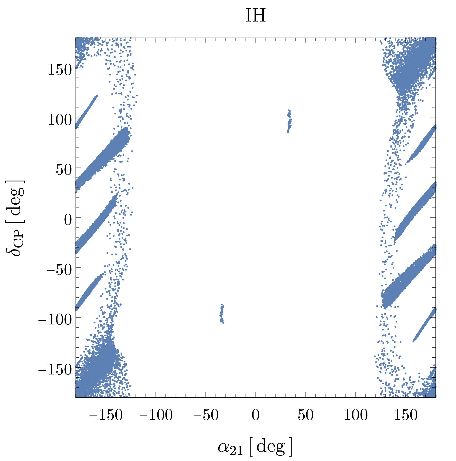
First of all, we have found no allowed region for the NH case. Fig. 1 shows the allowed regions for the $\tau$ and $\hat{g}$ for the IH case.

Refer to caption
Refer to caption
Figure 1: Allowed region of $\tau$ (left) and $\hat{g}=ge^{i\phi_{g}}$ (right) for inverted hierarchy. Each dot indicates the value that is consistent with the $3\sigma$ data of the neutrino oscillation experiments [115] summarized in Table 2.

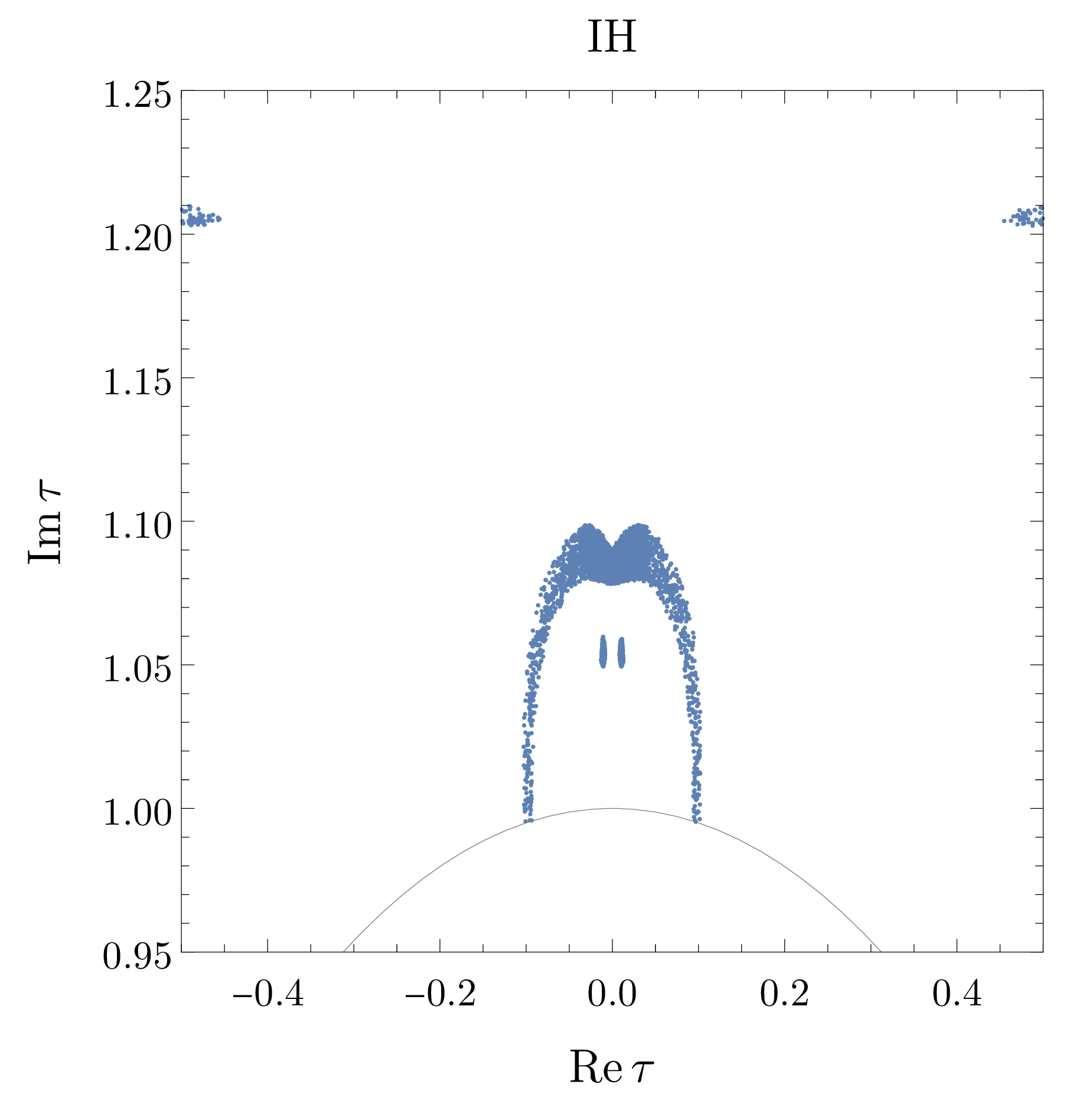
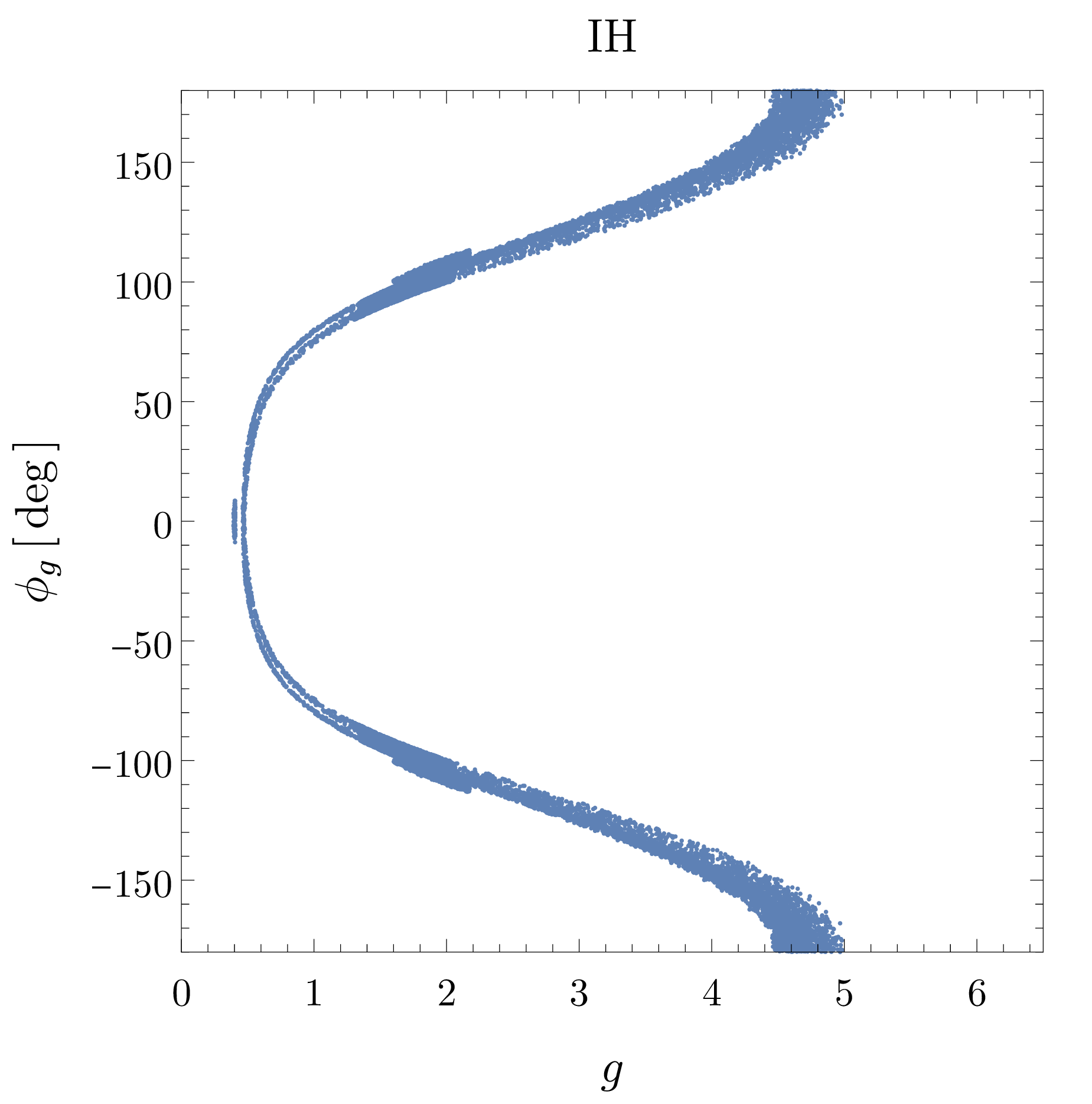
We found a specific pattern of the allowed values of $\tau$ and $\hat{g}$ is seen. The allowed value of $\tau$ is limited in $1.0\lesssim\mathrm{Im}\,\tau\lesssim 1.1$ and $|\mathrm{Re}\,\tau|\lesssim 0.1$, or $\mathrm{Im}\,\tau\sim 1.2$ and $|\mathrm{Re}\,\tau|\sim 0.5$. This is a different feature compared to the previous work, e.g., Ref. [11], where the allowed values of $\tau$ is distributed more widely. This difference comes from the unconventional pattern of the active neutrino mass matrix (3.10) given by Eqs. (3.8) and (3.9), which comes from additional Yukawa couplings between the right-handed neutrinos and $S_{+}$ in Eq. (2.31) and the VEV of $S_{+}$. Regarding $\hat{g}$, $g$ is distributed as $0.4\lesssim g\lesssim 5$. The phase $\phi_{g}$ can take any value in $[-180^{\circ},180^{\circ}]$, but it is given by a smooth function of $g$. Such behavior is in contrast to the results in Ref. [11]; in the literature, the allowed region for both $g$ and $\phi_{g}$ are more restricted.

Refer to caption
Refer to caption
Refer to caption
Figure 2: Predicted CP phases $\delta_{\rm CP}$ and $\alpha_{21}$ from the allowed parameter sets given in Fig. 1. The correlations between $\sin^{2}\theta_{23}$ and the CP phases (top-left and top-right) and the correlation between CP phases (bottom) are shown. The gray solid lines show the boundaries of the $3\sigma$ region of the experimental data.

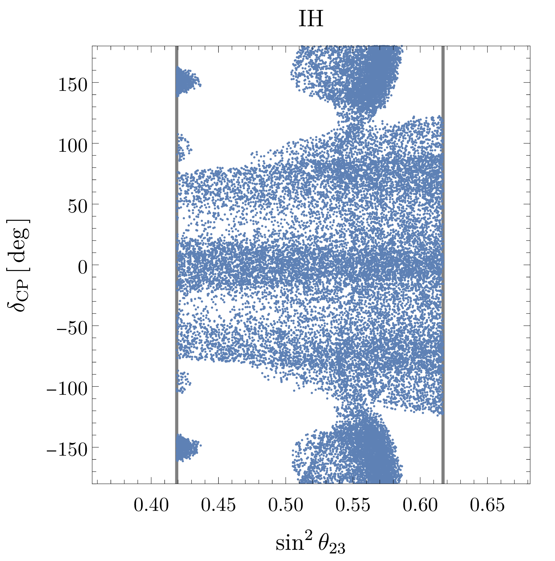
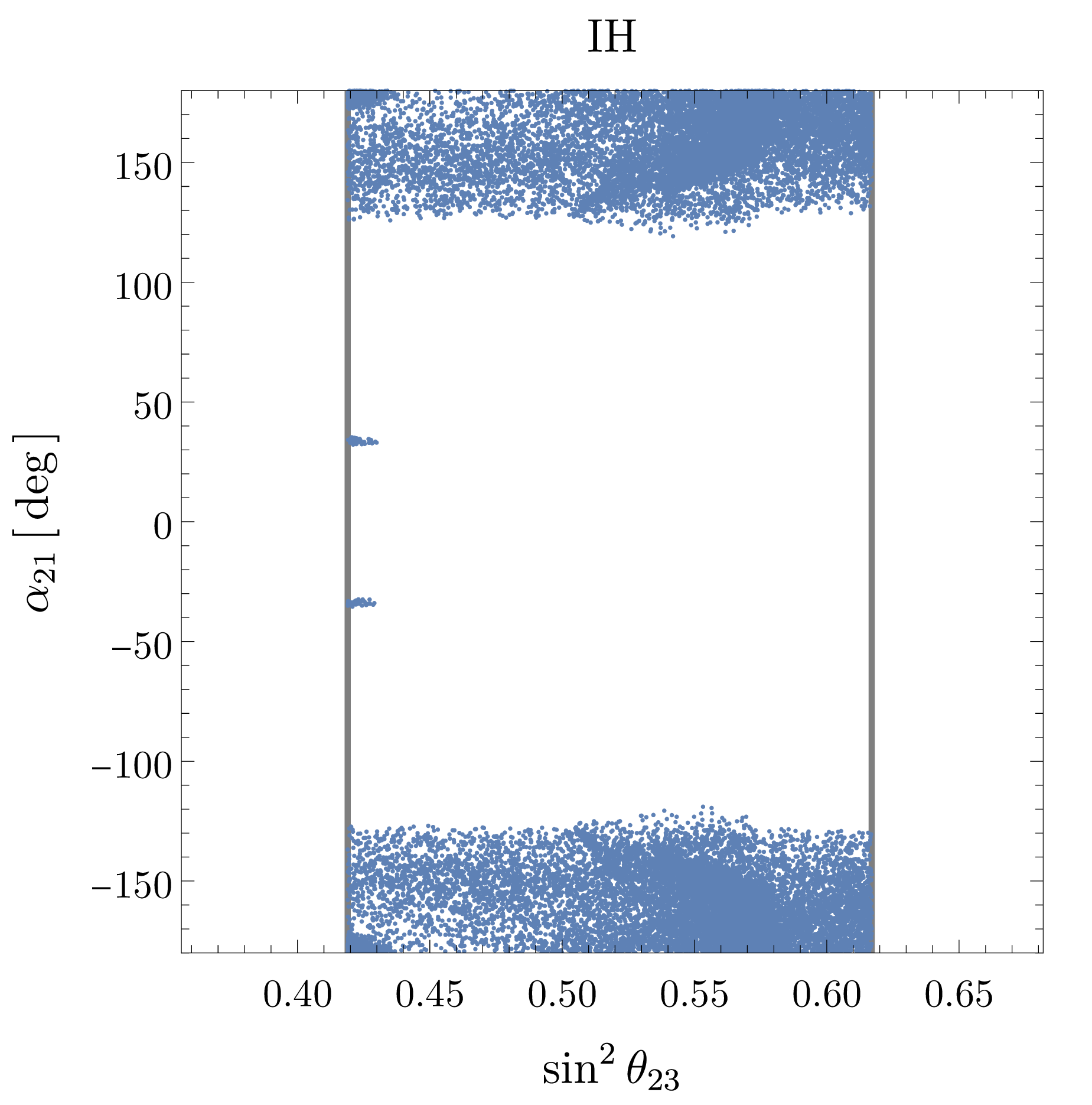
The discovered sets of the parameters lead to a new prediction for the CP phases, which is shown in Fig. 2. In the plot we show the correlation between $\sin^{2}\theta_{23}$ and the CP phases. For $\delta_{\rm CP}$, we found $|\delta_{\rm CP}|\lesssim 120^{\circ}$ for any value of $\sin^{2}\theta_{23}$ in the 3$\sigma$ range. If $\sin^{2}\theta_{23}\simeq 0.55$, on the other hand, then $\delta_{\rm CP}$ can take any values. Regarding $\alpha_{21}$, we found $|\alpha_{21}|\sim 120\text{--}180^{\circ}$ for any value of $\sin^{2}\theta_{23}$ in 3$\sigma$ range. An exception is $|\alpha_{21}|\sim 35^{\circ}$ for $\sin^{2}\theta_{23}\simeq 0.42\text{--}0.43$. Finally, we found no specific correlation between $\delta_{\rm CP}$ and $\alpha_{21}$, i.e., $|\alpha_{21}|\sim 120\text{--}180^{\circ}$ is predicted while various value of $\delta_{\rm CP}$ is possible. To summarize, only the IH is allowed and Fig. 2 is the prediction for the CP phases in our model.

Refer to caption
Refer to caption
Figure 3: Predicted effective neutrino mass of neutrinoless double beta decay as a function of the Majorana CP phase (left) and the Dirac CP phase (right), calculated from the results given in Fig. 2

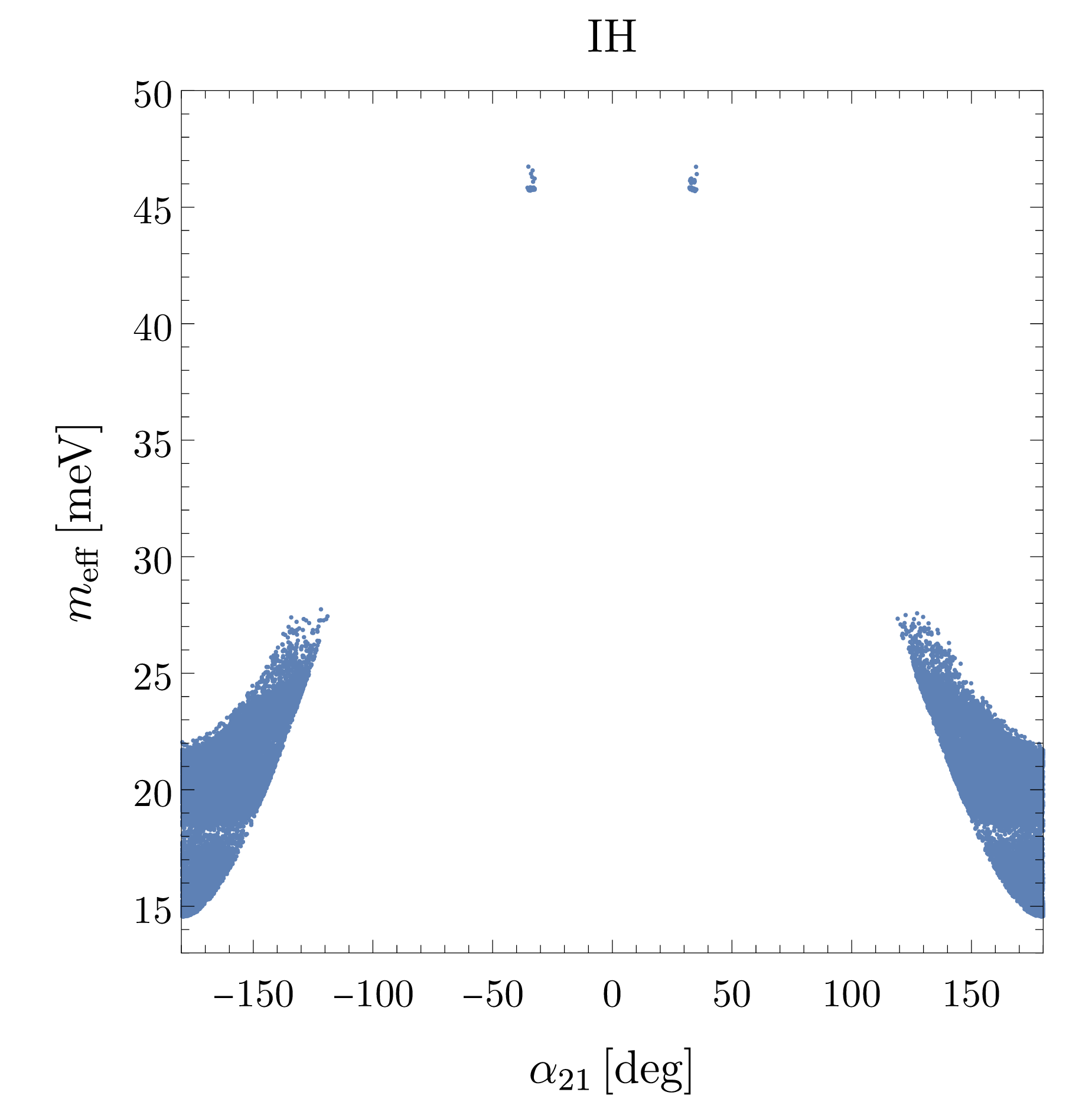
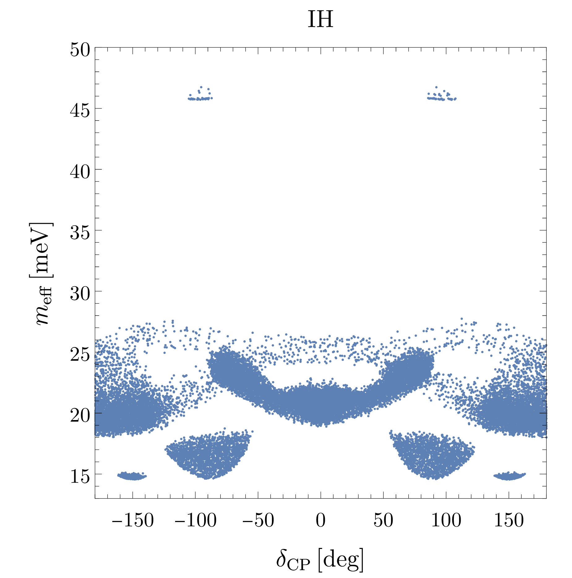
Another observable consequence of this model is the neutrinoless double beta decay $(A,Z)\to(A,Z+2)+2e^{-}$, which is a lepton number violating process in low-energy phenomena. See, e.g., Ref. [123] for review. The decay rate of the process is proportional to the effective neutrino mass-squared, which is given by

$\displaystyle m_{\rm eff}=\Bigl{|}\sum_{i}m_{i}U_{ei}^{2}\Bigr{|}\,.$ (3.25)

The current upper limit on the effective mass of neutrinoless double beta decay from KamLAND-Zen is 36–156 meV [124]. Note that the experimental upper bound on the effective mass is affected by the uncertainty of the nuclear matrix elements in the decay process. In the present model, one of the light neutrinos is massless and we have seen that the IH is allowed. Therefore, the effective neutrino mass is given by [125]

$\displaystyle m_{\rm eff}^{2}=c_{13}^{4}(m_{1}^{2}c_{12}^{4}+m_{2}^{2}s_{12}^{4}+2m_{1}m_{2}c_{12}^{2}s_{12}^{2}\cos\alpha_{21})\,.$ (3.26)

The result is shown in Fig. 3. We found $14~{}{\rm meV}\lesssim m_{\rm eff}\lesssim 28~{}{\rm meV}$ for the most parameter sets, where $\alpha_{21}\sim\pm 180^{\circ}$. One can see that it becomes as large as around 45–47 meV for $\alpha_{21}\sim\pm 35^{\circ}$, which can be understood from Eq. (3.26). Namely the term proportional to $\cos\alpha_{21}$ is constructive in this case. The resultant value $\order{10}~{}{\rm meV}$ of $m_{\rm eff}$ is the same as one shown in Ref. [125]. Since the model predicts a relatively large effective mass, neutrinoless double beta decay events may be observed in future experiments. If the CP phases are constrained, for instance, by considering the leptogenesis [126] in the present framework, then $m_{\rm eff}$ may be more restrictive. That would be another future work to pursue (see also the discussion in Sec. 4.5).

4 Inflation

$W_{\rm hyb}$ induces the $D$-term hybrid inflation. Motivated by the previous studies [102, 103], we consider the subcritical regime of hybrid inflation, where one of right-handed sneutrinos plays the role of the inflaton field. In the present case, however, the additional Majorana mass terms may disturb the dynamics during inflation. We will derive the inflaton potential and see how the additional terms affect the dynamics. In this section, we examine the impact of the heavy Majorana masses on the subcritical hybrid inflation scenario. To be concrete, we assume

$\displaystyle|M_{ij}|\ll|\lambda_{i}\langle S_{+}\rangle|\,.$ (4.1)

Under the assumption, we expect that the same inflation model is obtained as Ref. [103]. We will derive the upper bound for $M_{ij}$ quantitatively.

4.1 New field basis

We start with the basis given in the last paragraph of Sec. 2.2. At the global minimum, the mass matrix squared $M_{\mathrm{sc}}^{2}$ of the scalar sector in the basis $(\tilde{N}^{c}_{1},\tilde{N}^{c}_{2},\tilde{N}^{c}_{3},S_{-})$#4#4#4$\tilde{N}^{c}_{i}$ and $S_{\pm}$ are scalar components of the chiral superfield $N^{c}_{i}$ and $S_{\pm}$, respectively. is obtained as

$\displaystyle M_{\mathrm{sc}}^{2}$ $\displaystyle=\tilde{M}^{\dagger}\tilde{M}\,,$ (4.2)

where $\tilde{M}$ is equal to Eq. (3.8) without ‘hat’ symbol. Under the condition (4.1), the mass matrix is approximated as

$\displaystyle M_{\mathrm{sc}}^{2}$ $\displaystyle=\langle S_{+}\rangle^{2}\begin{pmatrix}|\lambda_{1}|^{2}&\lambda_{2}\lambda_{1}^{*}&\lambda_{3}\lambda_{1}^{*}&0\\ \lambda_{1}\lambda_{2}^{*}&|\lambda_{2}|^{2}&\lambda_{3}\lambda_{2}^{*}&0\\ \lambda_{1}\lambda_{3}^{*}&\lambda_{2}\lambda_{3}^{*}&|\lambda_{3}|^{2}&0\\ 0&0&0&\tilde{\lambda}^{2}\end{pmatrix}+\mathcal{O}(M_{ij}\lambda_{k}\langle S_{+}\rangle)\,,$ (4.3)

where

$\displaystyle\tilde{\lambda}\equiv\sqrt{\sum_{i}|\lambda_{i}|^{2}}$ (4.4)

and it can be approximately diagonalized by a unitary matrix $V$ as

$\displaystyle V^{\dagger}M_{\mathrm{sc}}^{2}V$ $\displaystyle=\langle S_{+}\rangle^{2}\begin{pmatrix}0&&&\\ &0&&\\ &&\tilde{\lambda}^{2}&\\ &&&\tilde{\lambda}^{2}\end{pmatrix}+\mathcal{O}(M_{ij}\lambda_{k}\langle S_{+}\rangle)\,,$ (4.5)
$\displaystyle V$ $\displaystyle\equiv\left(\begin{array}[]{@{}c:c@{}}W&\begin{matrix}0\\ 0\\ 0\end{matrix}\\ \hdashline\begin{matrix}0&0&0\end{matrix}&\frac{\lambda_{3}^{*}}{|\lambda_{3}|}\end{array}\right)\,,\quad W\equiv\begin{pmatrix}\frac{-\lambda_{3}|\lambda_{1}|}{\lambda_{1}\sqrt{\sum_{j\neq 2}|\lambda_{j}|^{2}}}&\frac{-\lambda_{2}\lambda_{1}^{*}}{\tilde{\lambda}\sqrt{\sum_{j\neq 2}|\lambda_{j}|^{2}|}}&\frac{|\lambda_{3}|\lambda_{1}^{*}}{\lambda_{3}^{*}\tilde{\lambda}}\\ 0&\sqrt{\frac{\sum_{j\neq 2}|\lambda_{j}|^{2}}{\tilde{\lambda}^{2}}}&\frac{|\lambda_{3}|\lambda_{2}^{*}}{\lambda_{3}^{*}\tilde{\lambda}}\\ \frac{|\lambda_{1}|}{\sqrt{\sum_{j\neq 2}|\lambda_{j}|^{2}}}&\frac{-\lambda_{2}\lambda_{3}^{*}}{\tilde{\lambda}\sqrt{\sum_{j\neq 2}|\lambda_{j}|^{2}}}&|\lambda_{3}|/\tilde{\lambda}\end{pmatrix}\,.$ (4.8)

Therefore, it is legitimate to use a new basis of $(N^{\prime c}_{1},N^{\prime c}_{2},N^{\prime c}_{3},S^{\prime}_{-})^{T}\equiv V^{\dagger}(N^{c}_{1},N^{c}_{2},N^{c}_{3},S_{-})^{T}$. In this basis, it is straightforward to find that $S^{\prime}_{\pm}$ only couple to $N^{\prime c}_{3}$. Then, the superpotential (2.31) is written as

$\displaystyle W_{\rm hyb}=\tilde{\lambda}S^{\prime}_{+}S^{\prime}_{-}N^{\prime c}_{3}+\frac{1}{2}M^{\prime}_{ij}N^{\prime c}_{i}N^{\prime c}_{j}\,,$ (4.9)

where $M^{\prime}\equiv W^{T}MW$ is a $3\times 3$ matrix of order $|M_{ij}|$. Therefore, $\phi\equiv\sqrt{2}\mathrm{Re}\,\tilde{N}^{\prime c}_{3}$ becomes the inflaton field [105, 103].

The parameter $\alpha$ can be taken to various values and different predictions for $n_{s}$ and $r$ are obtained accordingly, which is intensively analyzed in Ref. [103]. In the current study, we take

$\displaystyle\alpha$ $\displaystyle=2/3\,,~{}~{}~{}\tilde{\lambda}=0.959\times 10^{-3}\,,\quad\xi=(0.604\times 10^{16}\,\mathrm{GeV})^{2}\,,$ (4.10)

and $q=y=1$. Then the best-fit value of observed spectral index $n_{s}$, along with the tensor-to-scalar ratio $r\simeq 6\times 10^{-4}$, is obtained at the last 60 $e$-folds of the subcritical regime of the hybrid inflation [103]. With the parameters, the condition (4.1) gives

$\displaystyle|M^{\prime}_{ij}|\ll 10^{13}\,{\rm GeV}\,,$ (4.11)

where $\expectationvalue{S^{\prime}_{+}}=(\xi/(2/3)q(1+\tilde{\xi}))^{1/2}$ and $\tilde{\xi}\equiv\xi/2q$ has been used, which will be shown in the next subsection. In the following subsections, we will quantitatively examine the condition (4.11) to keep the inflaton dynamics unchanged. To keep the readable analytic expressions, we leave $\tilde{\lambda}$, $\xi$, $q$ and $y$ as they are.

4.2 The scalar potential

The scalar potential is given by [103],

$\displaystyle V$ $\displaystyle=V_{F}+V_{D}\,,$ (4.12)
$\displaystyle V_{F}$ $\displaystyle=\Bigl{(}-\frac{\Phi}{3}\Bigr{)}^{-1}\frac{3}{2}\bigl{[}\delta^{I\bar{J}}W_{I}\overline{W}_{\bar{J}}+\frac{1}{\Delta}\bigl{|}\delta^{I\bar{J}}W_{I}\Phi_{\bar{J}}-2W\bigr{|}^{2}+\frac{2}{\Phi}|W|^{2}\bigr{]}\,,$ (4.13)
$\displaystyle V_{D}$ $\displaystyle=\frac{y^{2}}{2}\Bigl{[}\Bigl{(}-\frac{\Phi}{3}\Bigr{)}^{-1}\frac{2q}{3}\bigl{(}|S^{\prime}_{+}|^{2}-|S^{\prime}_{-}|^{2}\bigr{)}-\xi\Bigr{]}^{2}\,,$ (4.14)

where $V_{F}$ and $V_{D}$ are $F$ and $D$-term potentials, respectively. Here $W_{I}\equiv\partial W/\partial z^{I}\,,\,\Phi_{I}\equiv\partial\Phi/\partial z^{I}\,$, and $\Delta\equiv\Phi-\delta^{I\bar{J}}\Phi_{I}\Phi_{\bar{J}}$, and $z^{I}$ shows the scalar component of $Z^{I}$. In the $D$-term potential, $y$ and $\xi\,(>0)$ are the gauge coupling and the Fayet-Iliopoulos (FI) term related to the local U(1). Due to the FI-term, $S^{\prime}_{+}$ acquires a VEV as $\langle S^{\prime}_{+}\rangle=(\xi/(2/3)q(1+\tilde{\xi}))^{1/2}$ at the global minimum.#5#5#5From Eq. (4.10), it is clear that $\expectationvalue*{S_{+}}\ll 1$. Then, $s\equiv\sqrt{2}|S^{\prime}_{+}|$ is identified with the waterfall field.

During inflation, we expect that the fields except for the inflaton and waterfall fields are stabilized at the origin. Thus the scalar potential during inflation is given as

$\displaystyle V(\phi,\,s)$ $\displaystyle\equiv V|_{\sqrt{2}\mathrm{Re}\tilde{N}^{\prime c}_{3}=\phi,\,\sqrt{2}|S^{\prime}_{+}|=s,\,\text{the others}=0}$
$\displaystyle=\Bigl{(}-\frac{\Phi(\phi,\,s)}{3}\Bigr{)}^{-1}\frac{3\phi^{2}}{4}\Bigl{[}\frac{\tilde{\lambda}^{2}}{2}s^{2}+\varDelta M^{2}(\phi,\,s)\Bigr{]}$
$\displaystyle\quad+\frac{y^{2}}{8}\Bigl{[}\Bigl{(}-\frac{\Phi(\phi,\,s)}{3}\Bigr{)}^{-1}\frac{2q}{3}s^{2}-2\xi\Bigr{]}^{2}\,,$ (4.15)

where $\Phi(\phi,\,s)\equiv-3+(s^{2}+\phi^{2})/2$. $\Delta M^{2}(\phi,s)$ is the term that originates in the Majorana mass term, which is given by

$\displaystyle\varDelta M^{2}(\phi,\,s)$ $\displaystyle\equiv\sum_{i=1}^{3}|M^{\prime}_{i3}|^{2}-|M^{\prime}_{33}|^{2}\frac{\phi^{2}}{12}\Bigl{(}-\frac{\Phi(\phi,\,s)}{3}\Bigr{)}^{-1}\,.$ (4.16)

4.3 Critical point

As in the literature [99, 100, 102, 105, 103], we focus on the dynamics of the subcritical regime of the hybrid inflation. First of all, the Majorana mass term shifts the critical point value of the hybrid inflation. The critical point value is determined by the mass squared of the waterfall field, which is given by

$\displaystyle m_{+}^{2}=m_{+,0}^{2}+\varDelta m_{+}^{2}\,,$ (4.17)

where

$\displaystyle m_{+,0}^{2}$ $\displaystyle\equiv qy^{2}\xi\bigl{(}\Psi(\phi)-1\bigr{)}\,,$ (4.18)
$\displaystyle\varDelta m_{+}^{2}$ $\displaystyle\equiv qy^{2}\xi\Psi(\phi)\frac{1}{3\tilde{\lambda}^{2}}\Bigl{(}-\frac{\Phi_{0}}{3}\Bigr{)}^{-1}$
$\displaystyle\quad\times\Bigl{[}\varDelta M^{2}(\phi,0)+|M^{\prime}_{33}|^{2}\frac{\phi^{2}}{12}\Bigl{(}-\frac{\Phi_{0}}{3}\Bigr{)}^{-1}\Bigr{]}\,,$ (4.19)
$\displaystyle\Psi(\phi)$ $\displaystyle\equiv\frac{\tilde{\lambda}^{2}}{2(2/3)^{2}qy^{2}\xi}\phi^{2}\,,\quad\Phi_{0}\equiv\Phi(\phi,0)\,.$ (4.20)

Here we have given the mass in a canonically normalized basis in accordance with Ref. [103]. Consequently, the critical point value $\phi_{c}$ is obtained by

$\displaystyle\phi_{c}^{2}$ $\displaystyle=\phi_{c,0}^{2}(1-\delta)+\mathcal{O}(M_{i3}^{\prime 4})\,,$ (4.21)

where $\phi_{c,0}^{2}={2(2/3)^{2}qy^{2}\xi}/{\tilde{\lambda}^{2}}$ [103] and

$\displaystyle\delta$ $\displaystyle\equiv\frac{2(2/3)^{2}}{\tilde{\lambda}^{2}}\frac{\varDelta m_{+}^{2}(\phi_{c,0})}{\phi_{c,0}^{2}}\,.$ (4.22)

Imposing $|\delta|\ll 1$, the upper bound on $|M^{\prime}_{i3}|$ is obtained as

$\displaystyle\sum_{i=1}^{2}|M^{\prime}_{i3}|^{2}$ $\displaystyle\ll 3\tilde{\lambda}^{2}-4qy^{2}\xi/9\simeq 3\times 10^{-7}\sim(1\times 10^{15}\,\mathrm{GeV})^{2}\,,$ (4.23)
$\displaystyle|M^{\prime}_{33}|^{2}$ $\displaystyle\ll\frac{(3\tilde{\lambda}^{2}-4qy^{2}\xi/9)^{2}}{3\tilde{\lambda}^{2}(3\tilde{\lambda}^{2}-8qy^{2}\xi/9)}\simeq 4\times 10^{-8}\sim(5\times 10^{14}\,\mathrm{GeV})^{2}\,.$ (4.24)

Those are weaker bounds compared to Eq. (4.11). Therefore, the critical point value is merely affected by the Majorana mass term.

4.4 Subcritical regime

Below the critical point, the waterfall field grows due to the tachyonic instability [127, 99] and soon relaxes to the local minimum $s_{\mathrm{min}}$ of the classical path.#6#6#6 We have confirmed that the one-loop potential dominates over the Majorana mass terms near the critical point under the condition (4.11). Thus, the dynamics around the critical point is the same as one studied in Ref. [103]. $s_{\mathrm{min}}$ is obtained by $\partial V(\phi,s)/\partial s^{2}=0$ as

$\displaystyle s_{\mathrm{min}}^{2}$ $\displaystyle=\frac{3\xi}{q}\frac{(-\Phi_{0}/3)}{1+\tilde{\xi}(1-\Psi(\phi))}$
$\displaystyle\quad\times\Biggl{[}1-\Psi(\phi)\Biggl{\{}1-\frac{\tilde{\xi}\bigl{[}1-\Psi(\phi)\bigr{]}(\Delta_{+}-\Delta_{-})-\Delta_{-}}{1+\tilde{\xi}\bigl{[}1-\Psi(\phi)(1+\Delta_{+})\bigr{]}}\Biggr{\}}\Biggr{]}\,,$ (4.25)

where

$\displaystyle\Delta_{\pm}$ $\displaystyle\equiv\Bigl{(}-\frac{\Phi_{0}}{3}\Bigr{)}^{-1}\frac{1}{3\tilde{\lambda}^{2}}\Bigl{[}\varDelta M^{2}(\phi,0)\pm|M^{\prime}_{33}|^{2}\frac{\phi^{2}}{12}\Bigl{(}-\frac{\Phi_{0}}{3}\Bigr{)}^{-1}\Bigr{]}\,.$ (4.26)

Consequently the potential in the subcritical regime can be expressed by a single field effective potential

$\displaystyle V_{\mathrm{sub}}(\phi)$ $\displaystyle\equiv V(\phi,\,s_{\mathrm{min}}(\phi))$
$\displaystyle=y^{2}\xi^{2}\Psi(\phi)\Biggl{[}1-\frac{\Psi(\phi)}{2}+\frac{1+\tilde{\xi}\{1-\Psi(\phi)\}}{3\tilde{\lambda}^{2}\tilde{\xi}}\Bigl{(}-\frac{\Phi_{0}}{3}\Bigr{)}^{-1}$
$\displaystyle\qquad\qquad\times\Bigl{[}\varDelta M^{2}(\phi,0)-|M^{\prime}_{33}|^{2}\frac{\phi^{2}}{12}\Bigl{(}-\frac{\Phi_{0}}{3}\Bigr{)}^{-1}\tilde{\xi}\{1-\Psi(\phi)\}\Bigr{]}\Biggr{]}+\mathcal{O}(M_{i3}^{\prime 4})$
$\displaystyle=y^{2}\xi^{2}\Psi(\phi)\Biggl{[}1-\frac{\Psi(\phi)}{2}+\frac{1}{3\tilde{\lambda}^{2}\tilde{\xi}}\Bigl{(}-\frac{\Phi_{0}}{3}\Bigr{)}^{-1}\varDelta M^{2}(\phi,0)\Biggr{]}+\mathcal{O}(M_{i3}^{\prime 4},\xi^{3})\,.$ (4.27)

In the last step, we have used $\xi\ll 1$. Therefore, $V_{\mathrm{sub}}$ reduces to the inflaton potential in Ref. [103] when

$\displaystyle|\varDelta M^{2}(\phi,0)|$ $\displaystyle\ll 3\tilde{\lambda}^{2}\tilde{\xi}\Bigl{(}-\frac{\Phi_{0}}{3}\Bigr{)}\Bigl{[}1-\frac{\Psi(\phi)}{2}\Bigr{]}\,,$ (4.28)

is satisfied. This condition gives rise to upper bounds on $|M^{\prime}_{i3}|$ as

$\displaystyle\sum_{i=1}^{2}|M^{\prime}_{i3}|^{2}$ $\displaystyle\ll 3\tilde{\xi}\tilde{\lambda}^{2}(1+\phi_{c,0}^{2}/6)/2\sim(2\times 10^{12}\,\mathrm{GeV})^{2}\,,$ (4.29)
$\displaystyle|M^{\prime}_{33}|^{2}$ $\displaystyle\ll 2\tilde{\xi}\tilde{\lambda}^{2}{(1-\phi_{c,0}^{2}/6)^{2}}/{|4-\phi_{c,0}^{2}|}\sim(9\times 10^{11}\,\mathrm{GeV})^{2}\,.$ (4.30)

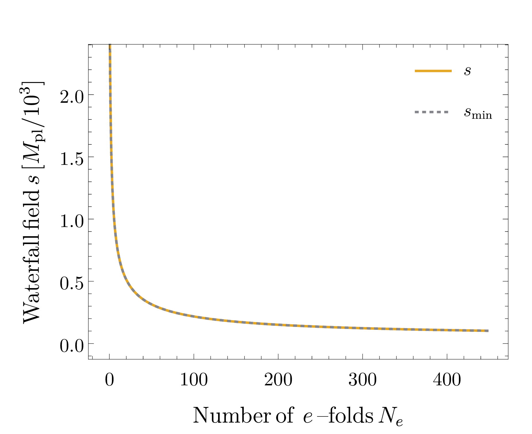
Those are a bit tighter than the condition (4.11). When the above conditions are satisfied, $s_{\mathrm{min}}$ is also in approximate agreement with the local minimum value of the waterfall field in Ref. [103],

$\displaystyle s_{\mathrm{min}}^{2}$ $\displaystyle=\frac{3\xi}{q}\Bigl{(}-\frac{\Phi_{0}}{3}\Bigr{)}\Bigl{[}1-\Psi(\phi)\Bigr{]}+\mathcal{O}(\xi\Delta_{-})\,.$ (4.31)

To summarize the inflaton dynamics is not affected if

$\displaystyle|M^{\prime}_{i3}|\ll 10^{12}\,\mathrm{GeV}\,,$ (4.32)

is satisfied.#7#7#7We have checked that the stability of the $\tilde{L}_{i}H_{u}$ direction, pointed out by Ref. [128], is guaranteed if $|M^{\prime}_{ij}|\lesssim 10^{18}\,{\rm GeV}$. In the next subsection, we will confirm the condition numerically.

4.5 Dynamics of scalar fields: numerical study

Refer to caption
Refer to caption
Refer to caption
Refer to caption
Figure 4: The time evolution of $s$, $\phi_{i}$, and $\tau_{i}$ $(i=1\text{--}3)$ as function of $e$-folds before the end of inflation. The parameters are given in Eq. (4.39) and $\hat{\Lambda}=10^{10}\,\mathrm{GeV}$. (Top-left) The waterfall field value $s$ (solid) given by the numerical solution and that of the analytical approximation $s_{\mathrm{min}}$ (dotted) are shown. (Top-right) The inflaton $\phi_{3}$ (solid) and $\tau_{3}$ (dashed) are given. (Bottom) $\phi_{i}$ (solid) and $\tau_{i}$ (dashed) for $i=1,2$ are shown.

The upper bound (4.32) is obtained under the assumption that the fields except for the inflaton and waterfall fields are stabilized at the origin during inflation. However, we need to investigate the validity of this assumption since the values of $\tilde{N}^{\prime c}_{1,2}$ and $\mathrm{Im}\,\tilde{N}^{\prime c}_{3}$ may grow to affect the dynamics of inflation depending on the value of the Majorana masses. We will check the stability of $\tilde{N}^{\prime c}_{1,2}$ and $\mathrm{Im}\,\tilde{N}^{\prime c}_{3}$ by solving the equations of motion of $\tilde{N}^{\prime c}_{i}$ and $S^{\prime}_{+}$ numerically and examine the condition (4.32) more quantitatively.

To this end, we define the relevant scalar fields as $\{\phi_{i},\,\tau_{i},\,s\}\equiv\varphi^{A}$ where#8#8#8Namely, $\phi_{3}=\phi$ is the inflaton field in the notation of this subsection.

$\displaystyle\phi_{i}\equiv\sqrt{2}\mathrm{Re}\,\tilde{N}^{\prime c}_{i}\,,\,\tau_{i}\equiv\sqrt{2}\mathrm{Im}\,\tilde{N}^{\prime c}_{i}\,.\,$ (4.33)

Then, the metric in terms of the field space of $\varphi^{A}$ is given by

$\displaystyle G_{AB}=\delta_{AB}\left\{\begin{array}[]{ll}K^{\rm m}_{N_{i}\bar{N}_{i}}&{\rm for}~{}\varphi^{A}=\phi_{i}\,,\tau_{i}\\ K^{\rm m}_{S^{+}\bar{S}^{+}}&{\rm for}~{}\varphi^{A}=s\end{array}\right.\,,$ (4.36)

where KZIZ¯J=2KzIz¯Jsubscript𝐾superscript𝑍𝐼superscript¯𝑍𝐽partial-derivativesuperscript𝑧𝐼1superscript¯𝑧𝐽1𝐾K_{Z^{I}\bar{Z}^{J}}=\partialderivative*{K}{z^{I}}{\bar{z}^{J}}. The equations of motion of $\varphi^{A}$ are

$\displaystyle\ddot{\varphi}^{A}+3H\dot{\varphi}^{A}+G^{AB}\frac{\partial V}{\partial\varphi^{B}}+\Gamma^{A}_{BC}\dot{\varphi}^{B}\dot{\varphi}^{C}=0\,.$ (4.37)

Here, dot denotes the time derivative and $H$ is the Hubble parameter that depends on $\varphi^{A}$ and $\dot{\varphi}^{A}$. $G^{AB}$ is the inverse of $G_{AB}$ and $\Gamma^{A}_{BC}$ is the connection defined by

$\displaystyle\Gamma^{A}_{BC}\equiv\frac{1}{2}G^{AD}(G_{DB,C}+G_{DC,B}-G_{BC,D})\,.$ (4.38)

For the numerical analysis, we take a benchmark point from the allowed region of $\tau$ and $\hat{g}$, which is given by

$\displaystyle\begin{split}\mathrm{Re}\,\tau&=8.88\times 10^{-4}\,,\quad\mathrm{Im}\,\tau=1.08\,,\\ g&=4.56\,,\quad\phi_{g}=-170^{\circ}\,.\end{split}$ (4.39)

With the parameters the corresponding neutrino mixing parameters are

$\displaystyle\begin{split}\sin^{2}\theta_{12}&=0.305\,,\quad\sin^{2}\theta_{13}=0.0224\,,\quad\sin^{2}\theta_{23}=0.572\,,\\ \delta_{\mathrm{CP}}&=-160^{\circ}\,,\quad\alpha_{21}=-163^{\circ}\,,\end{split}$ (4.40)

and $|M^{\prime}_{ij}|$ is obtained as

$\displaystyle|M^{\prime}_{ij}|$ $\displaystyle=\begin{pmatrix}5.59&3.56&9.75\\ 3.56&6.52&6.57\\ 9.75&6.57&3.53\end{pmatrix}\times 10^{9}\,\mathrm{GeV}\,\Bigl{(}\frac{\hat{\Lambda}}{10^{10}\,\mathrm{GeV}}\Bigr{)}\,.$ (4.41)

Since we are considering the subcritical regime, the initial values of $\phi$ and $s$ are set to $\phi^{2}_{\mathrm{init}}\equiv 0.98\phi_{c,0}^{2}$ and $s_{\mathrm{init}}\equiv s_{\mathrm{min}}(\phi_{\mathrm{init}})$, respectively, at the time $t=0$, while the other initial field values are set to zero. We have confirmed that similar trajectories of the scalar fields are obtained for slightly different the initial values of the inflaton and waterfall fields.#9#9#9The waterfall field value is much smaller than the inflaton one during inflation and the trajectory is almost straight along the inflaton field direction. Therefore, the trajectory of $\phi_{3}$-$s$ system has no additional impact on the curvature perturbation, which is already studied in Ref. [103].
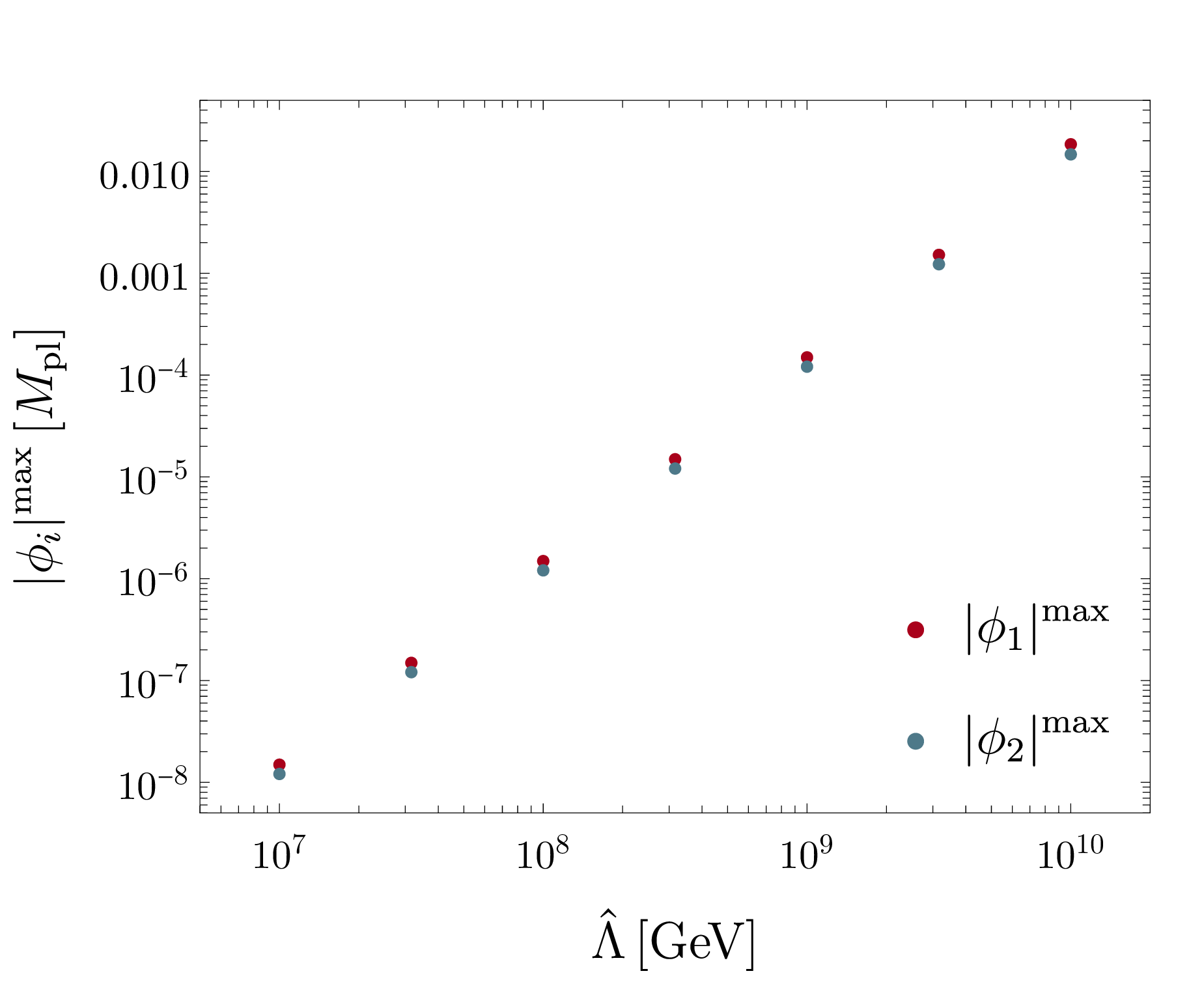
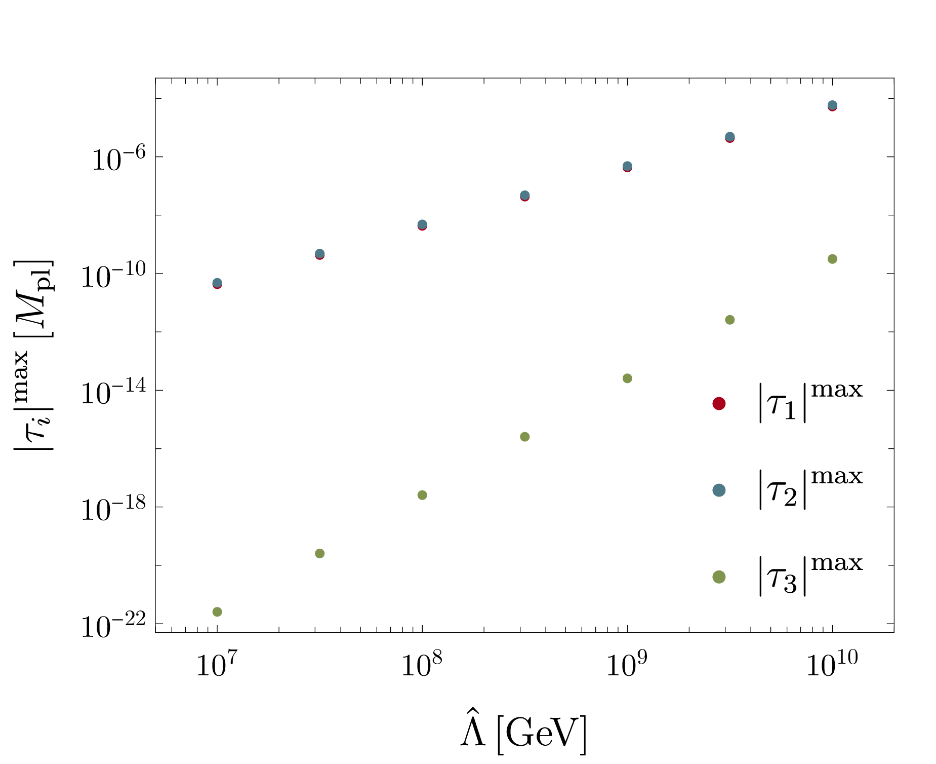
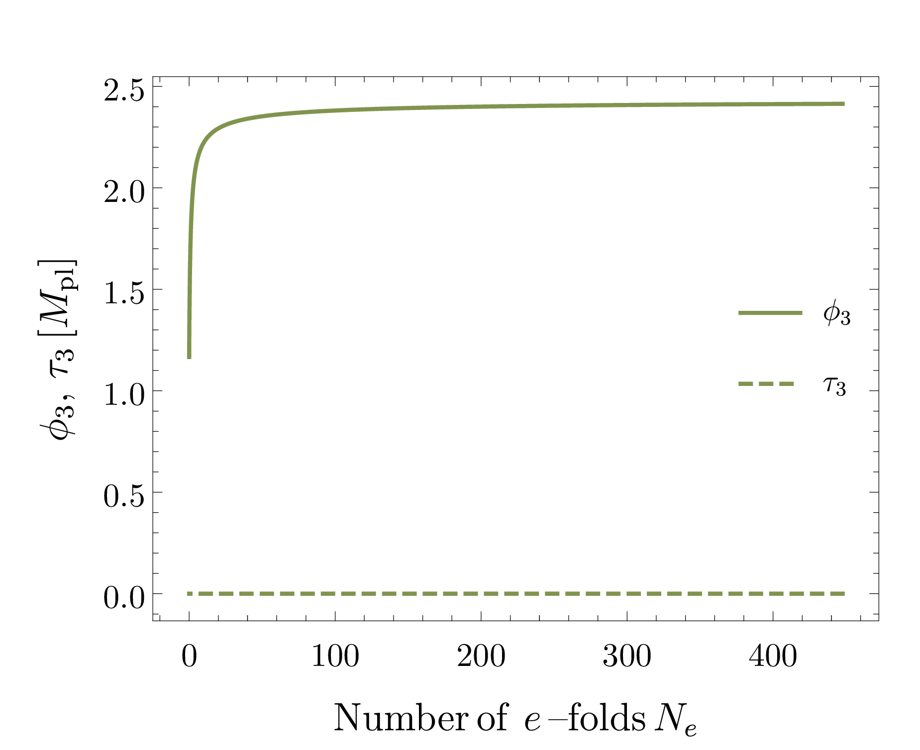
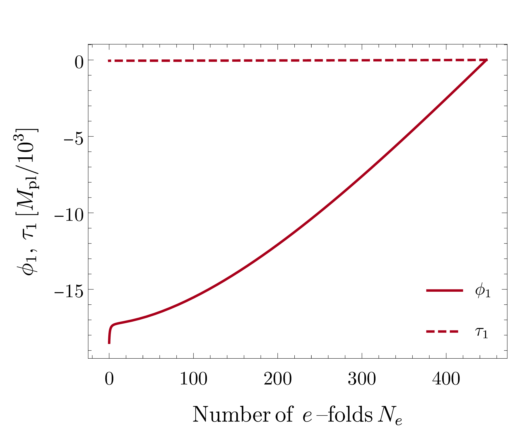
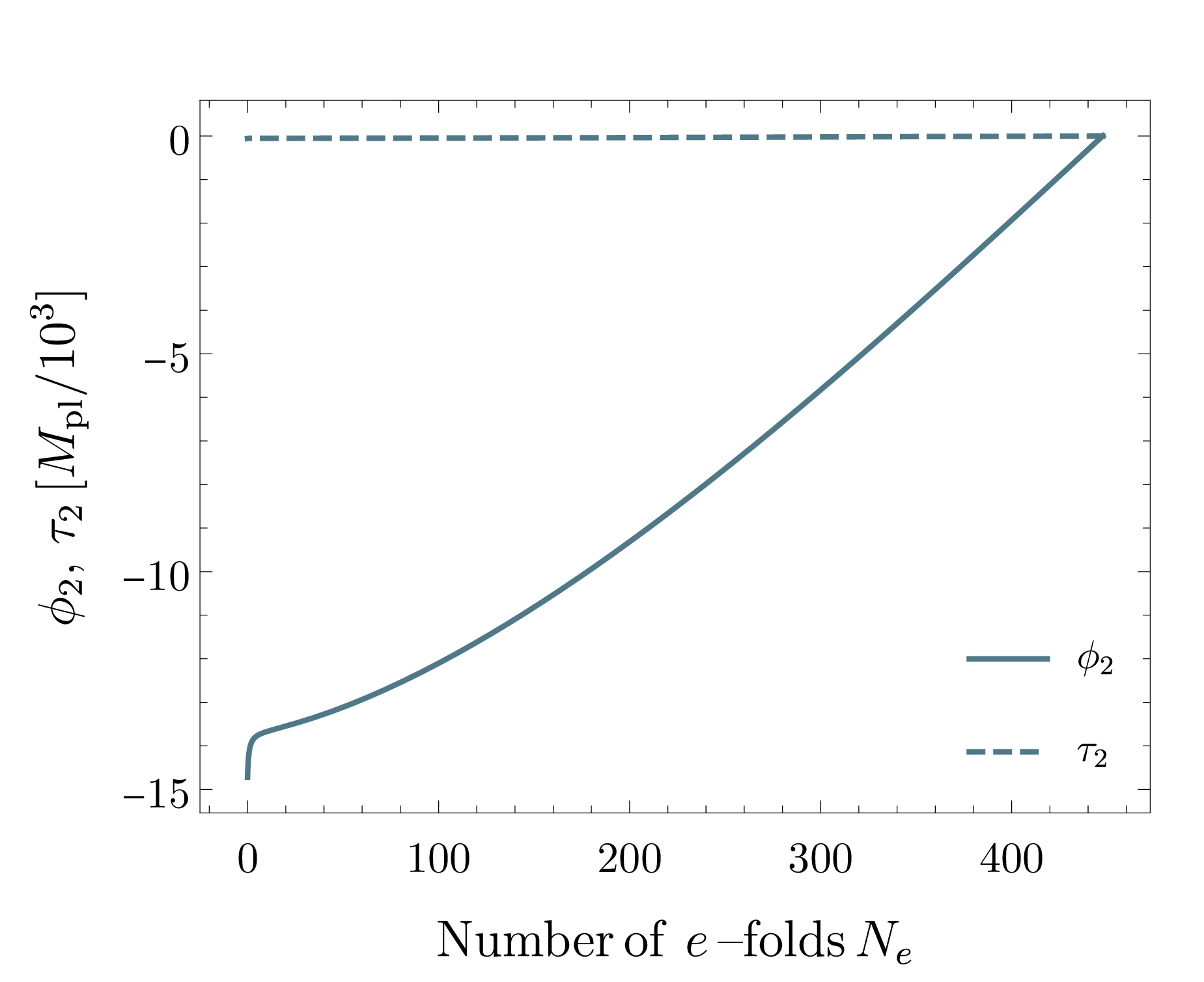
Refer to caption
Refer to caption
Figure 5: The maximum values of $\phi_{i}\,\,(i=1,2)$ (left) and $\tau_{i}\,\,(i=1\text{--}3)$ (right) during inflation as functions of $\Lambda$. Red, blue, and green points correspond to $i=1$, $2$, and $3$, respectively.

Fig. 4 shows the time evolution of $\varphi^{A}$ before the end of inflation as a function of the $e$-folds $N_{e}$ defined by

$\displaystyle N_{e}(t)=\int^{t_{\rm end}}_{t}dt^{\prime}H\,,$ (4.42)

where $t_{\rm end}$ is the time at the end of inflation. In the plot, $\hat{\Lambda}=10^{10}\,\mathrm{GeV}$ is taken to satisfy the condition (4.32) at a percent level. We confirmed that the trajectory of the waterfall field well agrees with the local minimum $s_{\rm min}$, given in Eq. (4.31). In addition, we found that the $\tau_{i}$ $(i=1\text{--}3)$ merely move during the inflation. On the other hand, $\phi_{1}$ and $\phi_{2}$ grow as large as $\order{\expectationvalue{s}}$ as seen in the figure.#10#10#10$\phi_{i}$ ($i=1,2$) are kicked by the term proportional to jRe(MijMj3)ϕiϕ3subscript𝑗superscriptsubscript𝑀𝑖𝑗subscript𝑀𝑗3subscriptitalic-ϕ𝑖subscriptitalic-ϕ3\sum_{j}\real(M_{ij}^{*}M_{j3})\phi_{i}\phi_{3}. The direction that $\phi_{i}$ is heading for depends on the sign of jRe(MijMj3)subscript𝑗superscriptsubscript𝑀𝑖𝑗subscript𝑀𝑗3\sum_{j}\real(M_{ij}^{*}M_{j3}). They are, however, still subdominant components in the scalar potential and they do not have any impact on the waterfall-inflaton dynamics. For smaller value of $\hat{\Lambda}$ we found that the field values of $\phi_{1}$ and $\phi_{2}$ reduce almost linearly, which is summarized in Fig. 5. Having confirmed the condition (4.32), we derived more quantitative bound,

$\displaystyle\hat{\Lambda}\lesssim 10^{10}\,\mathrm{GeV}\,,$ (4.43)

or equivalently

$\displaystyle|M^{\prime}_{i3}|\lesssim 10^{10}\,\mathrm{GeV}\,.$ (4.44)
Refer to caption
Refer to caption
Figure 6: Time evolution of $\phi_{1}$ and $\phi_{2}$ as function of the cosmic time $t$. Here $H_{c}\equiv H|_{\phi=\phi_{c}}\simeq 6.1\times 10^{12}\,\mathrm{GeV}$. The parameters are the same as Fig. 4.

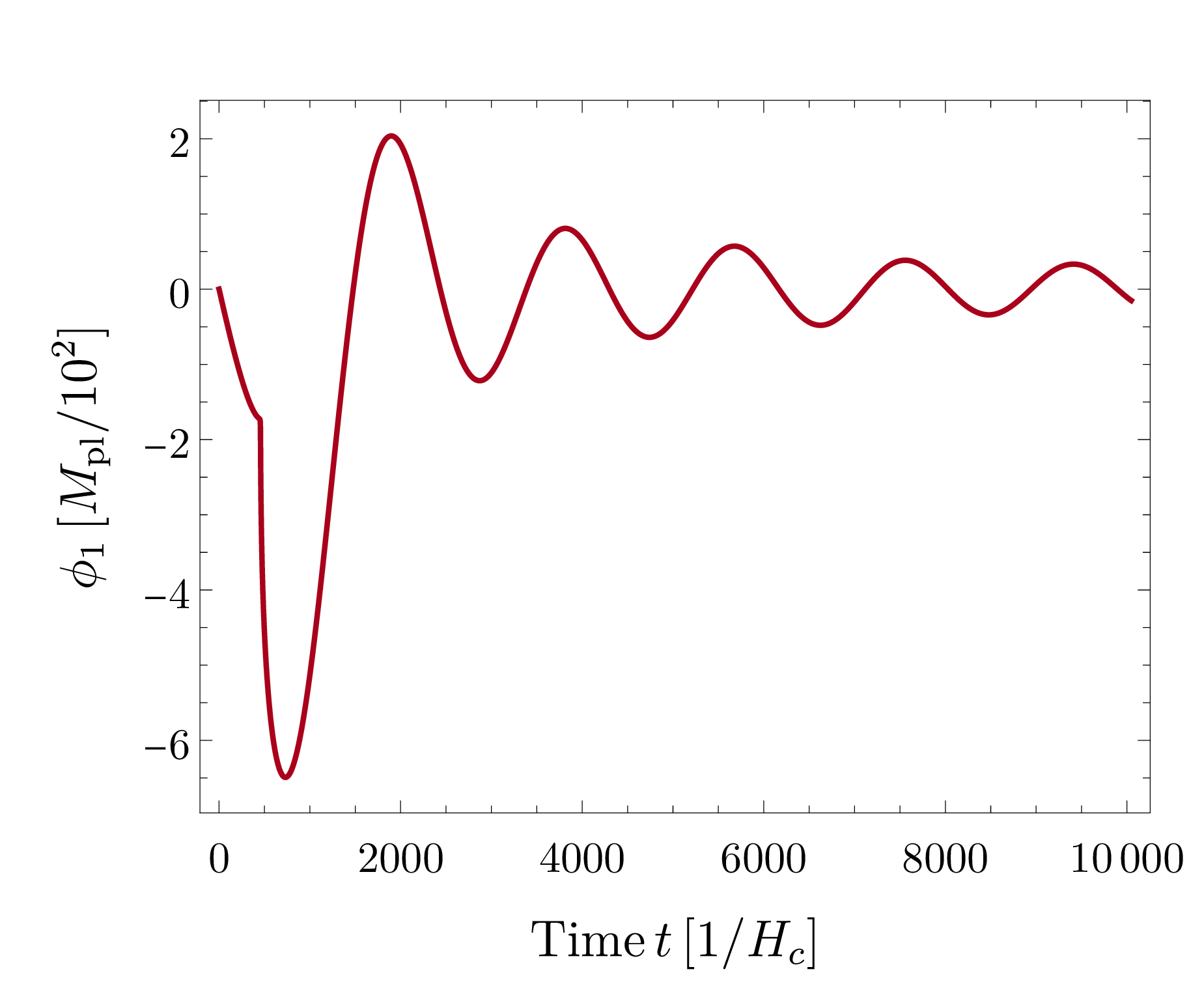
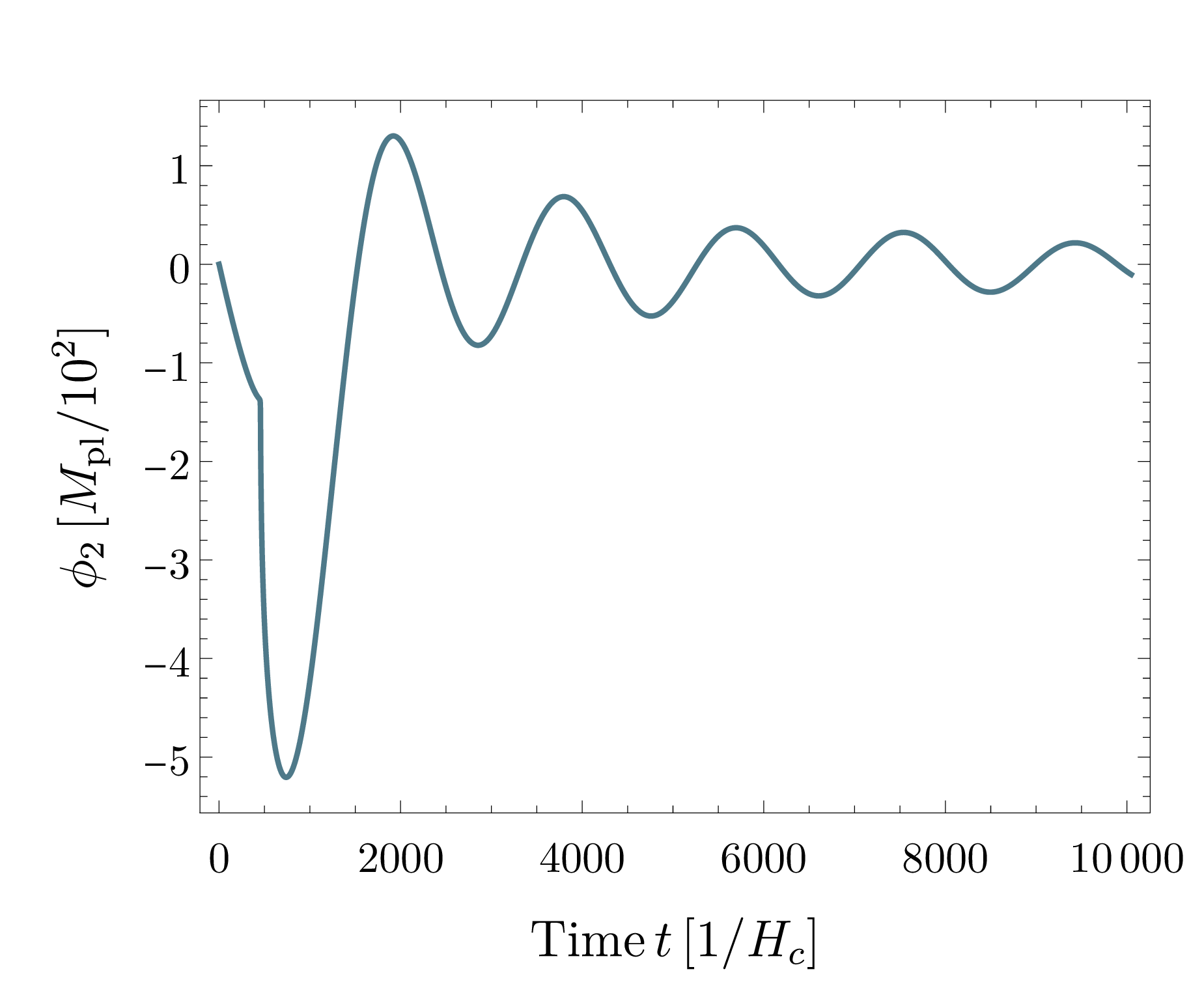
In the bottom panels of Fig. 4, the field growths of $\phi_{1}$ and $\phi_{2}$ get accelerated. This is because the Hubble parameter begins to decrease after the end of inflation since the inflaton field oscillates around the minimum to behave as a matter component. After that, the $\phi_{1}$ and $\phi_{2}$ start to oscillate with an angular frequency $\order{|M_{ij}|}$. We checked this behavior numerically, which is shown in Fig. 6. Here we have assumed that the inflaton field keeps the coherent oscillation. Realistically the inflaton field decays to leptons and Higgsinos or sleptons and Higgses and it reheats the universe. Then the radiation domination follows. Although $\phi_{1}$ and $\phi_{2}$ continue the coherent oscillation, we expect that they do not become the dominant component of the universe because their energy density is highly suppressed. In that case, non-thermal leptogenesis by the inflaton field works and it is expected to provide a sufficient number of lepton asymmetry [126, 128, 129, 130, 131, 132, 133, 134, 135, 136, 137, 138, 105]. The details depend on the model parameters and they are beyond the scope of our current study. We leave it for our future study.

5 Conclusion

We consider a supergravity model that has the modular $A_{4}$ symmetry. This model accommodates the MSSM augmented by three right-handed neutrino fields that have the Majorana masses. Additionally, two fields that are charged under a gauged U(1) are introduced. They couple to the right-handed neutrinos via the Yukawa interaction and consequently one of the scalar components plays a role of the waterfall field during inflation and acquires a VEV at the global minimum. With the extension, the pattern of the light neutrino mass, generated by the seesaw mechanism, changes and one of the light neutrinos becomes massless. On top of that, the modular $A_{4}$ symmetry restricts the mixing pattern. Comparing with the current observations regarding the neutrino mixings, we have found that only the IH case is allowed. The predicted Majorana phase is around $\pm 35^{\circ}$, the Dirac phase is $[-110^{\circ},-90^{\circ}],~{}[90^{\circ},110^{\circ}]$ and $0.42\lesssim\sin^{2}\theta_{23}\lesssim 0.43$, or the Majorana phase is $[-180^{\circ},-120^{\circ}],~{}[120^{\circ},180^{\circ}]$, the Dirac phase takes values in $[-180^{\circ},180^{\circ}]$ and $0.42\lesssim\sin^{2}\theta_{23}\lesssim 0.62$. The effective neutrino mass, which determines the decay rate of the neutrinoless double beta decay, is found to be around 14–28 meV and 45–47 meV. Such a relatively large effective mass of $\mathcal{O}(10)$ meV will be explored in future experiments.

The supergravity model we consider is based on a hybrid inflation model that has the subcritical inflation regime. Namely, inflation continues below the critical point. In the present model, the three right-handed sneutrinos are the candidates for the inflaton field. Compared to the inflation model studied in Ref. [103], the existence of the Majorana mass terms is a crucial difference, which may affect the inflation dynamics. Imposing the Majorana mass not to affect the inflation dynamics, we have revealed that only one of the right-handed sneutrinos turns out to couple to the waterfall field, then we have derived the upper bound for the Majorana mass scale analytically. We have confirmed the results numerically by solving the equations of motion for scalar fields. It is found the other right-handed sneutrinos grow as large as the VEV of the waterfall field. They are, however, negligible in the total energy density during the inflation if the Majorana mass scale is smaller than $\order{10^{10}}~{}{\rm GeV}$. Though their field values are much suppressed during inflation, the scalar fields continue to oscillate after inflation, which may affect the subsequent thermal history. For instance, they may contribute to the generation of the lepton asymmetry. The details depend on the parameter and we leave it for the future work.

Acknowledgments

We thank Tatsuo Kobayashi for valuable discussion at the early stage of this project and Takehiko Asaka for useful comments on the preprint. This work is supported by JST SPRING, Grant No. JPMJSP2135 (YG), JSPS KAKENHI Grant No. JP18H05542, JP20H01894, JSPS Core-to-Core Program Grant No. JPJSCCA20200002 (KI), and JSPS KAKENHI Grant No. 20H01898 (TY).

References

  • [1] Planck collaboration, Planck 2018 results. X. Constraints on inflation, Astron. Astrophys. 641 (2020) A10 [1807.06211].
  • [2] F. Feruglio, Are neutrino masses modular forms?, 1706.08749.
  • [3] MINOS collaboration, Measurement of Neutrino and Antineutrino Oscillations Using Beam and Atmospheric Data in MINOS, Phys. Rev. Lett. 110 (2013) 251801 [1304.6335].
  • [4] MINOS collaboration, Electron neutrino and antineutrino appearance in the full MINOS data sample, Phys. Rev. Lett. 110 (2013) 171801 [1301.4581].
  • [5] T2K collaboration, Measurement of neutrino and antineutrino oscillations by the T2K experiment including a new additional sample of $\nu_{e}$ interactions at the far detector, Phys. Rev. D 96 (2017) 092006 [1707.01048].
  • [6] T2K collaboration, Search for CP Violation in Neutrino and Antineutrino Oscillations by the T2K Experiment with $2.2\times 10^{21}$ Protons on Target, Phys. Rev. Lett. 121 (2018) 171802 [1807.07891].
  • [7] NOvA collaboration, Constraints on Oscillation Parameters from $\nu_{e}$ Appearance and $\nu_{\mu}$ Disappearance in NOvA, Phys. Rev. Lett. 118 (2017) 231801 [1703.03328].
  • [8] NOvA collaboration, New constraints on oscillation parameters from $\nu_{e}$ appearance and $\nu_{\mu}$ disappearance in the NOvA experiment, Phys. Rev. D 98 (2018) 032012 [1806.00096].
  • [9] T. Kobayashi, K. Tanaka and T.H. Tatsuishi, Neutrino mixing from finite modular groups, Phys. Rev. D 98 (2018) 016004 [1803.10391].
  • [10] J.C. Criado and F. Feruglio, Modular Invariance Faces Precision Neutrino Data, SciPost Phys. 5 (2018) 042 [1807.01125].
  • [11] T. Kobayashi, N. Omoto, Y. Shimizu, K. Takagi, M. Tanimoto and T.H. Tatsuishi, Modular A4 invariance and neutrino mixing, JHEP 11 (2018) 196 [1808.03012].
  • [12] T. Kobayashi, Y. Shimizu, K. Takagi, M. Tanimoto, T.H. Tatsuishi and H. Uchida, Finite modular subgroups for fermion mass matrices and baryon/lepton number violation, Phys. Lett. B 794 (2019) 114 [1812.11072].
  • [13] P.P. Novichkov, S.T. Petcov and M. Tanimoto, Trimaximal Neutrino Mixing from Modular A4 Invariance with Residual Symmetries, Phys. Lett. B 793 (2019) 247 [1812.11289].
  • [14] H. Okada and M. Tanimoto, Towards unification of quark and lepton flavors in $A_{4}$ modular invariance, Eur. Phys. J. C 81 (2021) 52 [1905.13421].
  • [15] T. Kobayashi, Y. Shimizu, K. Takagi, M. Tanimoto and T.H. Tatsuishi, New $A_{4}$ lepton flavor model from $S_{4}$ modular symmetry, JHEP 02 (2020) 097 [1907.09141].
  • [16] G.-J. Ding, S.F. King and X.-G. Liu, Modular A4 symmetry models of neutrinos and charged leptons, JHEP 09 (2019) 074 [1907.11714].
  • [17] H. Okada and Y. Orikasa, A radiative seesaw model in modular $A_{4}$ symmetry, 1907.13520.
  • [18] T. Kobayashi, Y. Shimizu, K. Takagi, M. Tanimoto and T.H. Tatsuishi, $A_{4}$ lepton flavor model and modulus stabilization from $S_{4}$ modular symmetry, Phys. Rev. D 100 (2019) 115045 [1909.05139].
  • [19] M.-C. Chen, S. Ramos-Sánchez and M. Ratz, A note on the predictions of models with modular flavor symmetries, Phys. Lett. B 801 (2020) 135153 [1909.06910].
  • [20] D. Zhang, A modular $A_{4}$ symmetry realization of two-zero textures of the Majorana neutrino mass matrix, Nucl. Phys. B 952 (2020) 114935 [1910.07869].
  • [21] T. Nomura, H. Okada and S. Patra, An inverse seesaw model with $A_{4}$ -modular symmetry, Nucl. Phys. B 967 (2021) 115395 [1912.00379].
  • [22] T. Kobayashi, T. Nomura and T. Shimomura, Type II seesaw models with modular $A_{4}$ symmetry, Phys. Rev. D 102 (2020) 035019 [1912.00637].
  • [23] X. Wang, Lepton flavor mixing and CP violation in the minimal type-(I+II) seesaw model with a modular $A_{4}$ symmetry, Nucl. Phys. B 957 (2020) 115105 [1912.13284].
  • [24] S.J.D. King and S.F. King, Fermion mass hierarchies from modular symmetry, JHEP 09 (2020) 043 [2002.00969].
  • [25] M. Abbas, Fermion masses and mixing in modular A4 Symmetry, Phys. Rev. D 103 (2021) 056016 [2002.01929].
  • [26] H. Okada and M. Tanimoto, Quark and lepton flavors with common modulus $\tau$ in $A_{4}$ modular symmetry, 2005.00775.
  • [27] T. Nomura and H. Okada, A linear seesaw model with $A_{4}$-modular flavor and local $U(1)_{B-L}$ symmetries, 2007.04801.
  • [28] T. Nomura and H. Okada, Modular $A_{4}$ symmetric inverse seesaw model with $SU(2)_{L}$ multiplet fields, 2007.15459.
  • [29] T. Asaka, Y. Heo and T. Yoshida, Lepton flavor model with modular $A_{4}$ symmetry in large volume limit, Phys. Lett. B 811 (2020) 135956 [2009.12120].
  • [30] K.I. Nagao and H. Okada, Lepton sector in modular A4 and gauged U(1)R symmetry, Nucl. Phys. B 980 (2022) 115841 [2010.03348].
  • [31] H. Okada and M. Tanimoto, Spontaneous CP violation by modulus $\tau$ in $A_{4}$ model of lepton flavors, JHEP 03 (2021) 010 [2012.01688].
  • [32] J. Gehrlein and M. Spinrath, Leptonic Sum Rules from Flavour Models with Modular Symmetries, JHEP 03 (2021) 177 [2012.04131].
  • [33] P.T.P. Hutauruk, D.W. Kang, J. Kim and H. Okada, Muon $g-2$ and neutrino mass explanations in a modular $A_{4}$ symmetry, 2012.11156.
  • [34] C.-Y. Yao, J.-N. Lu and G.-J. Ding, Modular Invariant $A_{4}$ Models for Quarks and Leptons with Generalized CP Symmetry, JHEP 05 (2021) 102 [2012.13390].
  • [35] F. Feruglio, V. Gherardi, A. Romanino and A. Titov, Modular invariant dynamics and fermion mass hierarchies around $\tau=i$, JHEP 05 (2021) 242 [2101.08718].
  • [36] T. Kobayashi, T. Shimomura and M. Tanimoto, Soft supersymmetry breaking terms and lepton flavor violations in modular flavor models, Phys. Lett. B 819 (2021) 136452 [2102.10425].
  • [37] M. Tanimoto and K. Yamamoto, Electron EDM arising from modulus $\tau$ in the supersymmetric modular invariant flavor models, JHEP 10 (2021) 183 [2106.10919].
  • [38] T. Nomura, H. Okada and Y. Orikasa, Quark and lepton flavor model with leptoquarks in a modular $A_{4}$ symmetry, Eur. Phys. J. C 81 (2021) 947 [2106.12375].
  • [39] I. de Medeiros Varzielas and J.a. Lourenço, Two A4 modular symmetries for Tri-Maximal 2 mixing, Nucl. Phys. B 979 (2022) 115793 [2107.04042].
  • [40] M.-C. Chen, V. Knapp-Perez, M. Ramos-Hamud, S. Ramos-Sanchez, M. Ratz and S. Shukla, Quasi–eclectic modular flavor symmetries, Phys. Lett. B 824 (2022) 136843 [2108.02240].
  • [41] H. Okada and Y.-h. Qi, Zee-Babu model in modular $A_{4}$ symmetry, 2109.13779.
  • [42] T. Nomura, H. Okada and Y.-h. Qi, Zee model in a modular $A_{4}$ symmetry, 2111.10944.
  • [43] X.-G. Liu and G.-J. Ding, Modular flavor symmetry and vector-valued modular forms, JHEP 03 (2022) 123 [2112.14761].
  • [44] S. Kikuchi, T. Kobayashi, H. Otsuka, M. Tanimoto, H. Uchida and K. Yamamoto, 4D modular flavor symmetric models inspired by higher dimensional theory, 2201.04505.
  • [45] T. Nomura and H. Okada, A radiative seesaw model in a supersymmetric modular $A_{4}$ group, 2201.10244.
  • [46] H. Otsuka and H. Okada, Radiative neutrino masses from modular $A_{4}$ symmetry and supersymmetry breaking, 2202.10089.
  • [47] T. Kobayashi, H. Otsuka, M. Tanimoto and K. Yamamoto, Lepton flavor violation, lepton $(g-2)_{\mu,\,e}$ and electron EDM in the modular symmetry, 2204.12325.
  • [48] Y.H. Ahn, S.K. Kang, R. Ramos and M. Tanimoto, Confronting the prediction of leptonic Dirac CP-violating phase with experiments, 2205.02796.
  • [49] M. Kashav and S. Verma, On Minimal realization of Topological Lorentz Structures with one-loop Seesaw extensions in A4 Modular Symmetry, 2205.06545.
  • [50] T. Nomura, H. Okada and Y. Shoji, $SU(4)_{C}\times SU(2)_{L}\times U(1)_{R}$ models with modular $A_{4}$ symmetry, 2206.04466.
  • [51] K. Ishiguro, H. Okada and H. Otsuka, Residual flavor symmetry breaking in the landscape of modular flavor models, 2206.04313.
  • [52] J. Gogoi, N. Gautam and M.K. Das, Neutrino masses and mixing in Minimal Inverse Seesaw using $A_{4}$ modular symmetry, 2207.10546.
  • [53] P.P. Novichkov, J.T. Penedo, S.T. Petcov and A.V. Titov, Modular A5 symmetry for flavour model building, JHEP 04 (2019) 174 [1812.02158].
  • [54] G.-J. Ding, S.F. King and X.-G. Liu, Neutrino mass and mixing with $A_{5}$ modular symmetry, Phys. Rev. D 100 (2019) 115005 [1903.12588].
  • [55] I. de Medeiros Varzielas and J.a. Lourenço, Two A5 modular symmetries for Golden Ratio 2 mixing, 2206.14869.
  • [56] H.P. Nilles, S. Ramos-Sánchez and P.K.S. Vaudrevange, Eclectic Flavor Groups, JHEP 02 (2020) 045 [2001.01736].
  • [57] G.-J. Ding, S.F. King, C.-C. Li and Y.-L. Zhou, Modular Invariant Models of Leptons at Level 7, JHEP 08 (2020) 164 [2004.12662].
  • [58] C.-C. Li, X.-G. Liu and G.-J. Ding, Modular symmetry at level 6 and a new route towards finite modular groups, JHEP 10 (2021) 238 [2108.02181].
  • [59] H. Ohki, S. Uemura and R. Watanabe, Modular flavor symmetry on a magnetized torus, Phys. Rev. D 102 (2020) 085008 [2003.04174].
  • [60] H. Okada and M. Tanimoto, CP violation of quarks in $A_{4}$ modular invariance, Phys. Lett. B 791 (2019) 54 [1812.09677].
  • [61] H. Kuranaga, H. Ohki and S. Uemura, Modular origin of mass hierarchy: Froggatt-Nielsen like mechanism, JHEP 07 (2021) 068 [2105.06237].
  • [62] S. Kikuchi, T. Kobayashi, M. Tanimoto and H. Uchida, Mass matrices with CP phase in modular flavor symmetry, 2206.08538.
  • [63] S. Kikuchi, T. Kobayashi, M. Tanimoto and H. Uchida, Texture zeros of quark mass matrices at fixed point $\tau=\omega$ in modular flavor symmetry, 2207.04609.
  • [64] S. Kikuchi, T. Kobayashi, K. Nasu, H. Otsuka, S. Takada and H. Uchida, Modular symmetry of soft supersymmetry breaking terms, 2203.14667.
  • [65] T. Kobayashi, Y. Shimizu, K. Takagi, M. Tanimoto, T.H. Tatsuishi and H. Uchida, $CP$ violation in modular invariant flavor models, Phys. Rev. D 101 (2020) 055046 [1910.11553].
  • [66] I. de Medeiros Varzielas, M. Levy and Y.-L. Zhou, Symmetries and stabilisers in modular invariant flavour models, JHEP 11 (2020) 085 [2008.05329].
  • [67] G.-J. Ding, F. Feruglio and X.-G. Liu, Automorphic Forms and Fermion Masses, JHEP 01 (2021) 037 [2010.07952].
  • [68] K. Ishiguro, T. Kobayashi and H. Otsuka, Landscape of Modular Symmetric Flavor Models, JHEP 03 (2021) 161 [2011.09154].
  • [69] P.P. Novichkov, J.T. Penedo and S.T. Petcov, Modular flavour symmetries and modulus stabilisation, JHEP 03 (2022) 149 [2201.02020].
  • [70] F.J. de Anda, S.F. King and E. Perdomo, $SU(5)$ grand unified theory with $A_{4}$ modular symmetry, Phys. Rev. D 101 (2020) 015028 [1812.05620].
  • [71] T. Kobayashi, Y. Shimizu, K. Takagi, M. Tanimoto and T.H. Tatsuishi, Modular $S_{3}$-invariant flavor model in SU(5) grand unified theory, PTEP 2020 (2020) 053B05 [1906.10341].
  • [72] X. Du and F. Wang, SUSY breaking constraints on modular flavor $S_{3}$ invariant SU(5) GUT model, JHEP 02 (2021) 221 [2012.01397].
  • [73] Y. Zhao and H.-H. Zhang, Adjoint SU(5) GUT model with modular $S_{4}$ symmetry, JHEP 03 (2021) 002 [2101.02266].
  • [74] P. Chen, G.-J. Ding and S.F. King, SU(5) GUTs with A4 modular symmetry, JHEP 04 (2021) 239 [2101.12724].
  • [75] S.F. King and Y.-L. Zhou, Twin modular S4 with SU(5) GUT, JHEP 04 (2021) 291 [2103.02633].
  • [76] G.-J. Ding, S.F. King and C.-Y. Yao, Modular $S_{4}\times SU(5)$ GUT, Phys. Rev. D 104 (2021) 055034 [2103.16311].
  • [77] G.-J. Ding, S.F. King and J.-N. Lu, SO(10) models with A4 modular symmetry, JHEP 11 (2021) 007 [2108.09655].
  • [78] T. Kobayashi, S. Nishimura, H. Otsuka, M. Tanimoto and K. Yamamoto, Generalized Matter Parities from Finite Modular Symmetries, 2207.14014.
  • [79] T. Nomura and H. Okada, A modular $A_{4}$ symmetric model of dark matter and neutrino, Phys. Lett. B 797 (2019) 134799 [1904.03937].
  • [80] T. Nomura and H. Okada, A two loop induced neutrino mass model with modular $A_{4}$ symmetry, Nucl. Phys. B 966 (2021) 115372 [1906.03927].
  • [81] H. Okada and Y. Orikasa, Modular $S_{3}$ symmetric radiative seesaw model, Phys. Rev. D 100 (2019) 115037 [1907.04716].
  • [82] T. Nomura, H. Okada and O. Popov, A modular $A_{4}$ symmetric scotogenic model, Phys. Lett. B 803 (2020) 135294 [1908.07457].
  • [83] H. Okada and Y. Orikasa, Neutrino mass model with a modular $S_{4}$ symmetry, 1908.08409.
  • [84] H. Okada and Y. Shoji, A radiative seesaw model with three Higgs doublets in modular $A_{4}$ symmetry, Nucl. Phys. B 961 (2020) 115216 [2003.13219].
  • [85] K.I. Nagao and H. Okada, Modular A4 symmetry and light dark matter with gauged U(1)B$-$L, Phys. Dark Univ. 36 (2022) 101039 [2108.09984].
  • [86] T. Kobayashi, H. Okada and Y. Orikasa, Dark matter stability at fixed points in a modular $A_{4}$ symmetry, 2111.05674.
  • [87] T. Asaka, Y. Heo, T.H. Tatsuishi and T. Yoshida, Modular $A_{4}$ invariance and leptogenesis, JHEP 01 (2020) 144 [1909.06520].
  • [88] M.K. Behera, S. Mishra, S. Singirala and R. Mohanta, Implications of A4 modular symmetry on neutrino mass, mixing and leptogenesis with linear seesaw, Phys. Dark Univ. 36 (2022) 101027 [2007.00545].
  • [89] S. Mishra, Neutrino mixing and Leptogenesis with modular $S_{3}$ symmetry in the framework of type III seesaw, 2008.02095.
  • [90] M. Kashav and S. Verma, Broken scaling neutrino mass matrix and leptogenesis based on A4 modular invariance, JHEP 09 (2021) 100 [2103.07207].
  • [91] H. Okada, Y. Shimizu, M. Tanimoto and T. Yoshida, Modulus $\tau$ linking leptonic CP violation to baryon asymmetry in A4 modular invariant flavor model, JHEP 07 (2021) 184 [2105.14292].
  • [92] A. Dasgupta, T. Nomura, H. Okada, O. Popov and M. Tanimoto, Dirac Radiative Neutrino Mass with Modular Symmetry and Leptogenesis, 2111.06898.
  • [93] M.K. Behera and R. Mohanta, Linear Seesaw in A5’ Modular Symmetry With Leptogenesis, Front. in Phys. 10 (2022) 854595 [2201.10429].
  • [94] D.W. Kang, J. Kim, T. Nomura and H. Okada, Natural mass hierarchy among three heavy Majorana neutrinos for resonant leptogenesis under modular $A_{4}$ symmetry, 2205.08269.
  • [95] G.-J. Ding, S.F. King, J.-N. Lu and B.-Y. Qu, Leptogenesis in $SO(10)$ Models with $A_{4}$ Modular Symmetry, 2206.14675.
  • [96] A.A. Starobinsky, A New Type of Isotropic Cosmological Models Without Singularity, Adv. Ser. Astrophys. Cosmol. 3 (1987) 130.
  • [97] V.F. Mukhanov and G.V. Chibisov, Quantum Fluctuations and a Nonsingular Universe, JETP Lett. 33 (1981) 532.
  • [98] W. Buchmuller, V. Domcke and K. Kamada, The Starobinsky Model from Superconformal D-Term Inflation, Phys. Lett. B 726 (2013) 467 [1306.3471].
  • [99] W. Buchmuller, V. Domcke and K. Schmitz, The Chaotic Regime of D-Term Inflation, JCAP 11 (2014) 006 [1406.6300].
  • [100] W. Buchmuller and K. Ishiwata, Grand Unification and Subcritical Hybrid Inflation, Phys. Rev. D 91 (2015) 081302 [1412.3764].
  • [101] R. Kallosh, A. Linde and D. Roest, Superconformal Inflationary $\alpha$-Attractors, JHEP 11 (2013) 198 [1311.0472].
  • [102] K. Ishiwata, Superconformal Subcritical Hybrid Inflation, Phys. Lett. B 782 (2018) 367 [1803.08274].
  • [103] Y. Gunji and K. Ishiwata, Subcritical hybrid inflation in a generalized superconformal model, Phys. Rev. D 104 (2021) 123545 [2104.02248].
  • [104] R. de Adelhart Toorop, F. Feruglio and C. Hagedorn, Finite Modular Groups and Lepton Mixing, Nucl. Phys. B 858 (2012) 437 [1112.1340].
  • [105] Y. Gunji and K. Ishiwata, Leptogenesis after superconformal subcritical hybrid inflation, JHEP 09 (2019) 065 [1906.04530].
  • [106] S. Ferrara, R. Kallosh, A. Linde, A. Marrani and A. Van Proeyen, Superconformal Symmetry, NMSSM, and Inflation, Phys. Rev. D 83 (2011) 025008 [1008.2942].
  • [107] P. Minkowski, $\mu\to e\gamma$ at a Rate of One Out of $10^{9}$ Muon Decays?, Phys. Lett. B 67 (1977) 421.
  • [108] T. Yanagida, Horizontal gauge symmetry and masses of neutrinos, Conf. Proc. C 7902131 (1979) 95.
  • [109] T. Yanagida, Horizontal Symmetry and Masses of Neutrinos, Prog. Theor. Phys. 64 (1980) 1103.
  • [110] M. Gell-Mann, P. Ramond and R. Slansky, Complex Spinors and Unified Theories, Conf. Proc. C 790927 (1979) 315 [1306.4669].
  • [111] P. Ramond, The Family Group in Grand Unified Theories, in International Symposium on Fundamentals of Quantum Theory and Quantum Field Theory, 2, 1979 [hep-ph/9809459].
  • [112] S.L. Glashow, The Future of Elementary Particle Physics, NATO Sci. Ser. B 61 (1980) 687.
  • [113] Planck collaboration, Planck 2018 results. VI. Cosmological parameters, Astron. Astrophys. 641 (2020) A6 [1807.06209].
  • [114] S. Vagnozzi, E. Giusarma, O. Mena, K. Freese, M. Gerbino, S. Ho et al., Unveiling $\nu$ secrets with cosmological data: neutrino masses and mass hierarchy, Phys. Rev. D 96 (2017) 123503 [1701.08172].
  • [115] I. Esteban, M.C. Gonzalez-Garcia, M. Maltoni, T. Schwetz and A. Zhou, The fate of hints: updated global analysis of three-flavor neutrino oscillations, JHEP 09 (2020) 178 [2007.14792].
  • [116] C. Jarlskog, Commutator of the Quark Mass Matrices in the Standard Electroweak Model and a Measure of Maximal $CP$ Nonconservation, Phys. Rev. Lett. 55 (1985) 1039.
  • [117] S.M. Bilenky, S. Pascoli and S.T. Petcov, Majorana neutrinos, neutrino mass spectrum, CP violation and neutrinoless double beta decay. 1. The Three neutrino mixing case, Phys. Rev. D 64 (2001) 053010 [hep-ph/0102265].
  • [118] J.F. Nieves and P.B. Pal, Rephasing invariant CP violating parameters with Majorana neutrinos, Phys. Rev. D 64 (2001) 076005 [hep-ph/0105305].
  • [119] J.A. Aguilar-Saavedra and G.C. Branco, Unitarity triangles and geometrical description of CP violation with Majorana neutrinos, Phys. Rev. D 62 (2000) 096009 [hep-ph/0007025].
  • [120] I. Girardi, S.T. Petcov and A.V. Titov, Predictions for the Majorana CP Violation Phases in the Neutrino Mixing Matrix and Neutrinoless Double Beta Decay, Nucl. Phys. B 911 (2016) 754 [1605.04172].
  • [121] G.F. Giudice and A. Romanino, Split supersymmetry, Nucl. Phys. B 699 (2004) 65 [hep-ph/0406088].
  • [122] G.F. Giudice and A. Strumia, Probing High-Scale and Split Supersymmetry with Higgs Mass Measurements, Nucl. Phys. B 858 (2012) 63 [1108.6077].
  • [123] H. Päs and W. Rodejohann, Neutrinoless Double Beta Decay, New J. Phys. 17 (2015) 115010 [1507.00170].
  • [124] KamLAND-Zen collaboration, First Search for the Majorana Nature of Neutrinos in the Inverted Mass Ordering Region with KamLAND-Zen, 2203.02139.
  • [125] T. Asaka and T. Yoshida, Resonant leptogenesis at TeV-scale and neutrinoless double beta decay, JHEP 09 (2019) 089 [1812.11323].
  • [126] M. Fukugita and T. Yanagida, Baryogenesis Without Grand Unification, Phys. Lett. B 174 (1986) 45.
  • [127] T. Asaka, W. Buchmuller and L. Covi, False vacuum decay after inflation, Phys. Lett. B 510 (2001) 271 [hep-ph/0104037].
  • [128] K. Nakayama, F. Takahashi and T.T. Yanagida, Viable Chaotic Inflation as a Source of Neutrino Masses and Leptogenesis, Phys. Lett. B 757 (2016) 32 [1601.00192].
  • [129] F. Björkeroth, S.F. King, K. Schmitz and T.T. Yanagida, Leptogenesis after Chaotic Sneutrino Inflation and the Supersymmetry Breaking Scale, Nucl. Phys. B 916 (2017) 688 [1608.04911].
  • [130] H. Murayama, H. Suzuki, T. Yanagida and J. Yokoyama, Chaotic inflation and baryogenesis by right-handed sneutrinos, Phys. Rev. Lett. 70 (1993) 1912.
  • [131] H. Murayama, H. Suzuki, T. Yanagida and J. Yokoyama, Chaotic inflation and baryogenesis in supergravity, Phys. Rev. D 50 (1994) R2356 [hep-ph/9311326].
  • [132] H. Murayama and T. Yanagida, Leptogenesis in supersymmetric standard model with right-handed neutrino, Phys. Lett. B 322 (1994) 349 [hep-ph/9310297].
  • [133] K. Hamaguchi, H. Murayama and T. Yanagida, Leptogenesis from N dominated early universe, Phys. Rev. D 65 (2002) 043512 [hep-ph/0109030].
  • [134] J.R. Ellis, M. Raidal and T. Yanagida, Sneutrino inflation in the light of WMAP: Reheating, leptogenesis and flavor violating lepton decays, Phys. Lett. B 581 (2004) 9 [hep-ph/0303242].
  • [135] S. Antusch, M. Bastero-Gil, S.F. King and Q. Shafi, Sneutrino hybrid inflation in supergravity, Phys. Rev. D 71 (2005) 083519 [hep-ph/0411298].
  • [136] S. Antusch, M. Bastero-Gil, K. Dutta, S.F. King and P.M. Kostka, Chaotic Inflation in Supergravity with Heisenberg Symmetry, Phys. Lett. B 679 (2009) 428 [0905.0905].
  • [137] K. Kadota and J. Yokoyama, D-term inflation and leptogenesis by right-handed sneutrino, Phys. Rev. D 73 (2006) 043507 [hep-ph/0512221].
  • [138] K. Nakayama, F. Takahashi and T.T. Yanagida, Chaotic Inflation with Right-handed Sneutrinos after Planck, Phys. Lett. B 730 (2014) 24 [1311.4253].