Morpho—A programmable environment for shape optimization and shapeshifting problems

Abstract

An emerging theme across many domains of science and engineering is materials that change shape, often dramatically. Determining their structure involves solving a shape optimization problem where a given energy functional is minimized with respect to the shape of the domain and auxiliary fields describing the structure. Such problems are very challenging to solve and there is a lack of suitable simulation tools that are both readily accessible and general purpose. To address this gap, we present Morpho, an open-source programmable environment, and demonstrate its versatility by showcasing three applications to different areas of soft matter physics—swelling hydrogels, complex fluids that form aspherical droplets, to soap films and membranes—and advise on broader uses.

Numerous domains of scientific research involve the solution of shape optimization and evolution problems: soft robots able to change their shape [1, 2, 3, 4, 5]; complex fluids, particulate matter and liquid crystals with free boundaries [6, 7, 8, 9, 10, 11, 12, 13]; systems where mechanical properties emerge from the structure [14, 15, 16]; active biological materials and membranes that are internally driven [17, 18, 19, 20, 21, 22, 23]; multiphase systems; gels [24, 25]; responsive polymeric materials [26, 27, 14], computational differential geometry [28], etc. to name a few. Cutting across many of these applications is the idea of shape as a programmable quantity [29, 27, 14] where a material or system is guided to a desired final configuration by local structure and an applied external influence such as a magnetic field or a chemical cue. In each of these scenarios, some energy functional must be minimized with respect to the shape of the system of interest together with other quantities such as electric or magnetic fields and also subject to imposed constraints.

In this Article, we introduce a programmable environment, Morpho, that aims to solve the following class of problems. Suppose we have a domain, $C=\bigcup_{i}c_{i}$ composed of subdomains $c_{i}$, in $n$ dimensional space. On $C$ are defined zero or more scalar or tensor fields, $\mathbf{q}$. The goal is to optimize a given energy functional with respect to the shape of the domain and the field values,

$$F=\sum_{i}\int_{c_{i}}f_{i}(\mathbf{q},\nabla\mathbf{q},...)d^{n}x+\sum_{i}\int_{\partial c_{i}}g_{i}(\mathbf{q},\nabla\mathbf{q},...)d^{n-1}x,$$

subject to global (integral) constraints,

$$\sum_{i}\int_{c_{i}}h_{i}(\mathbf{q},\nabla\mathbf{q})d^{n}x=0,$$

together with local constraints $u_{k}(\mathbf{q},\nabla\mathbf{q})=0$. Here, $f_{i}$, $g_{i}$, $h_{i}$ and $u_{k}$ are scalar functions of $\mathbf{q}$ and its gradients; these may differ by subdomain. The constraint set could also include inequality constraints such as limitations on the shape including mutual inter-penetrability between elements or excluding the mesh from encroaching on a certain region.

Numerous important problems lie in the class just described. For example, the shape of a soap film locally minimizes the area due to surface tension. In a compact geometry, i.e., a soap bubble, the volume may either be considered as fixed (implying a global constraint) or established by balancing the pressure difference inside and outside the droplet against the surface force. Non-compact geometries also can occur, where the shape of the boundary is prescribed, as in a soap film suspended by a wire.

We briefly review a number of other techniques that are used to solve shape optimization problems. Phase field methods [30, 31] use an auxiliary scalar field called the phase-field, that smoothly interpolates between the interior and exterior of a shape. Phase field methods are straightforward to implement, but resolving sharp features such as cusps that may arise in such problems can be difficult. Level set methods [32] represent the free boundary of the system as a contour or a level set of a scalar function defined in a higher dimensional space. An advantage of this is that changes in topology, such as the coalescence of two fluid droplets, can be easily handled. Formulating the optimization problem for a particular problem requires sophisticated techniques, however, and enforcement of constraints can be challenging.

In contrast, Morpho uses an explicit discretization of the problem domain and associated quantities. From these, Morpho is able to evaluate the objective function of interest as well as its gradients and Hessian with respect to mesh and field degrees of freedom. A number of algorithms for constrained optimization are then available within the Morpho environment to perform the optimization using these quantities. The approach is similar in spirit to the highly successful Surface Evolver (SE) software [33, 34]. Originally designed for minimal surface computations, SE has been adapted to many other uses. Surface Evolver’s success in part comes from its interactive, re-programmable and versatile nature, with direct applicability to arbitrary problems. Nonetheless, SE works with surfaces only and does not support optimization with respect to field quantities. Further, mesh quality control in SE requires user intervention, including manual refinement and coarsening steps. We significantly address these limitations in Morpho.

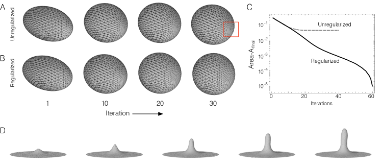
Figure 1: Soap films and membranes. Optimization of a soap film from an initial ellipsoidal configuration under surface tension at fixed enclosed volume: A without regularization and B with regularization. In the absence of regularization, vertices near the end of the solution become bunched together (highlighted region). C Residual area as a function of iteration showing that the unregularized solution converges on an incorrect solution. D Simulated drawing of a tether from a circular disk of bilayer membrane under the Helfrich energy.

From the user’s perspective, Morpho provides a very flexible, object-oriented environment for shape optimization. A user may work with the program interactively or by supplying a script to be run, written in a simple but powerful dynamic programming language similar to Python. The language is modular, thus supporting user-defined libraries and customization, and enables specification of a problem to closely correspond to the mathematical problem statement. Documentation is available through online help in interactive mode, a manual and a website. Convenient interactive visualization is provided through a companion application morphoview.

In the remainder of the paper, we describe a number of illustrative example applications of Morpho. First, we solve a classic problem, the shape of a soap film under surface tension at fixed volume. This example illustrates a key innovation of our work, which is the use of auxiliary functionals to automatically control mesh quality, improving the quality and accuracy of the solution. We then use Morpho to resolve the shape of anisotropic liquid crystal fluid droplets or tactoids in 2D and 3D, illustrating combined shape and field minimization. Finally, we study hydrogels swelling under confinement to illustrate the sophisticated use of constraints. We conclude with a discussion of Morpho’s feature set, its potential applicability to other research areas and avenues for future development. Further details of the environment and its implementation, together with additional information about the applications presented here are then provided in Methods.

I Results

I.1 Example 1: Minimal surfaces and membranes

An important class of problems include finding surfaces that minimize an energy functional. As we note in the introduction, a soap film minimizes the area,

$$F=\int_{C}dA,$$ (1)

where the domain $C$ is a surface embedded in $\mathbb{R}^{3}$. Because the minimizer of (1) vanishes to a point, typical problems involving soap films involve constraints. For example, the total volume enclosed in a compact soap film may be fixed, or the boundary may be specified. A related problem is to find the shape of a membrane, such as that enclosing a biological cell, which minimizes the Helfrich energy [35, 36, 37],

$$F=\sigma\int_{C}dA+\kappa\int_{C}\left(H-H_{0}\right)^{2}dA+K_{G}\int_{C}KdA+\lambda\int_{\partial C}dl,$$ (2)

where $H$ is the local mean curvature, $H_{0}$ is a locally preferred mean curvature, $K$ is the Gaussian curvature and $\sigma$, $\kappa$, $K_{G}$ and $\lambda$ are (material dependent) constants.

While these problems are quite simple to state, they enable us to explore some of the numerical subtleties of shape optimization problems before turning to more complex applications. An ubiquitous challenge is that the initial geometry specified by the user may prove to be very different from the solution, which could have a different topology, for example, or include features that are not hinted at in the starting point. Hence, shape optimization necessitates some form of adaptive mesh control. Strategies to maintain mesh quality include splitting elements where the solution is poorly resolved, merging elements where there is excessive detail, or redistributing elements to improve their density in regions of interest. Morpho provides support for all of these.

As an illustration, we show in Fig. 1 an initially ellipsoidal mesh that is relaxed back to a sphere under surface tension using a gradient descent scheme with line searches (See Methods). Figs. 1A and 1B show intermediate snapshots of the system in the first few iterations with and without mesh control, respectively; Fig. 1C shows the area of the system as a function of iteration number. As is evident, without mesh control, the system converges spuriously on an incorrect solution. Inspection of the solution (see red highlighted region in Fig. 1A) reveals why this occurs: mesh points at the ends of the ellipsoids are becoming bunched together. To explain this, we use an elementary result from differential geometry, that the gradient of the area with respect to a point on the surface locally lies in the direction of the surface normal. Hence, the target problem is under-determined; the tangential distribution of the vertices is not fully specified by the functional of interest.

To repair the situation, we supplement the problem (1) with an auxiliary regularization problem that penalizes differences in area between adjacent elements. This new problem is co-minimized together with the original problem; in practice we find only occasional regularization steps are necessary. With such steps, the algorithm converges correctly on a spherical solution as seen in Fig. 1C. In more complex problems, the continuous regularization scheme presented here can be supplemented with occasional discrete refinement steps, i.e., splitting or merging elements.

As an illustration of the use of Morpho’s mesh control features to solve a more challenging problem, in Fig. 1D we show the shape and formation of a tether from an initial disk-shaped patch of lipid membrane with fixed boundary. Such tethers occur in many biologically-relevant scenarios involving lipid bi-layers including micro-manipulation experiments on artificial vesicles as well as the Golgi apparatus[38]. The disk is subject to localized indentation, drawing out a cylindrical tether beyond a certain displacement.

I.2 Example 2: Liquid crystal tactoids

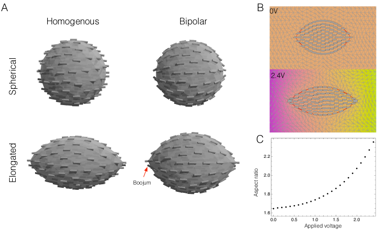
Figure 2: Nematic liquid crystal tactoids. A Three dimensional tactoid morphologies that occur in various parameter regimes. B Initial and final 2D tactoid shapes in the presence of an electric field. C Equilibrium aspect ratio as a function of applied voltage.

In contrast to isotropic fluids, anisotropic fluids can support elastic deformation, orientationally dependent surface tension and other physical effects that make non-spherical equilibrium droplet shapes possible. A commonly-encountered example of such a fluid is a nematic liquid crystal (NLC), which is composed of long, rigid molecules that tend to align locally in some preferred direction. These materials are commercially important for display and electro-optic applications, as well as emerging technologies such as chemical and biological sensors.

One way of mathematically describing these materials is through a unit vector field $\mathbf{n}(\mathbf{r})$ known as the director field, which specifies the average direction in which the molecules align at a location $\mathbf{r}$. To determine the equilibrium shape of a droplet $C$, the functional to be minimized in three dimensions is the free energy,

$$F= \int_{C}\left[\frac{1}{2}K_{11}\left(\nabla\cdot\mathbf{n}\right)^{2}+K_{22}(\mathbf{n}\cdot\nabla\times\mathbf{n})^{2}\right.$$

$$\quad+\left.K_{33}\left|\mathbf{n}\times\nabla\times\mathbf{n}\right|^{2}\right]\differential V$$

$$+\sigma\int_{\partial C}\differential A-\frac{W}{2}\int_{\partial C}\left(\mathbf{n}\cdot\mathbf{t}\right)^{2}\differential A,$$ (3)

where the various contributions to the energy are as follows: the first term corresponds to liquid crystal elasticity, with three constants $K_{11}$, $K_{22}$ and $K_{33}$ measuring the cost of splay, twist and bend deformations, respectively [39]; the second term is the surface tension with associated constant $\sigma$; and the final term imposes a preferred orientation at the boundary, a phenomenon known as anchoring. If the anchoring coefficient, $W>0$, the director, $\mathbf{n}$, prefers to align with the local tangent to the surface, $\mathbf{t}$.

The functional (3) is to be minimized with respect to the shape of the domain $C$ and the configuration of the director field $\mathbf{n}$ subject to a volume constraint,

$$\int_{C}\differential V=V_{0},$$

and a local constraint,

$$\mathbf{n}\cdot\mathbf{n}=1.$$

By introducing a length scale derived from the volume of the droplet $V^{1/3}$ and defining a mean elastic constant $\bar{K}=\frac{1}{3}\sum K_{ii}$, the above expression can be nondimensionalized. The solution is then a function of some dimensionless parameters $\kappa=\bar{K}/\sigma V^{1/3}$, the ratio of elastic forces to surface tension, $\omega=W/\sigma$, the ratio of anchoring energy to surface tension, and the reduced elastic constants $k_{ii}=K_{ii}/\bar{K},i\in\{1,2,3\}$.

In Figure 2A, we show paradigmatic solutions that illustrate the variety of possible morphologies. The local orientation of the director field is depicted using cylinders. For $\kappa\ll 1$, the surface tension holds the droplet in a spherical shape; as $\kappa\gtrapprox 1$ the droplet elongates to form a spindle shape. The director field also undergoes a transition: for $\omega<\omega_{o}(\kappa)$ elasticity overcomes anchoring leading to a homogenous director field; for $\omega>\omega_{0}(\kappa)$ the director aligns with the surface producing a bipolar configuration. The critical anchoring energy for these transitions has been predicted from a scaling theory [40]; here we obtain the solutions by direct optimization.

As well as elastic anisotropy, liquid crystals also exhibit dielectric anisotropy, whereby the dielectric tensor $\epsilon=\epsilon_{\perp}I_{3}+\epsilon_{a}\mathbf{n}\otimes\mathbf{n}$ depends on the local orientation of the director field $\mathbf{n}$. Here, $\epsilon_{\perp}$ is the component of the dielectric tensor perpendicular to $\mathbf{n}$, $I_{3}$ is the $3\times 3$ identity matrix and $\epsilon_{a}=\epsilon_{\parallel}-\epsilon_{\perp}$ is the dielectric anisotropy. The dielectric anisotropy has a number of physical consequences. At low frequency, if $\epsilon_{a}>0$ the director tends to reorient to align with an applied electric field. At optical frequencies, dielectric anisotropy implies birefringence. The combination of electrical switchability and optical activity facilitates the creation of switchable electro-optic devices such as displays.

To predict the effect of an electric field on the shape of a droplet of nematic, the free energy (3) must be supplemented by an additional term,

$$F_{\text{el}}=-\frac{1}{2}\int\mathbf{D}\cdot\mathbf{E}\ \differential V.$$ (4)

Here, $\mathbf{E}=-\nabla\phi$ is the electric field with $\phi$ being the electric potential, and $\mathbf{D}=\epsilon\mathbf{E}$. To find the equilibrium solution, we must minimize (3)+(4) as well as solve for the electric potential $\phi$. In Figure 2B, we show equilibrium solutions for increasing potential differences in two dimensions. The aspect ratio of the droplet is plotted in Fig. 2C showing elongation as the electric field is increased until, eventually, the solution becomes unstable.

These two scenarios highlight the rich possibilities for shape change that arise in complex fluids. Many further extensions of the present examples are possible in Morpho: Certain liquid crystal materials, for instance, adopt a spontaneously twisted structure and are known as cholesterics [39, 11]. Such materials can easily be simulated by incorporating an additional term in (3). Alternative theoretical formulations of liquid crystal elasticity [39, 41] exist and can readily be used within the program. Additional physics can be included by formulation and inclusion of an appropriate energy functional.

I.3 Example 3: Swelling hydrogels

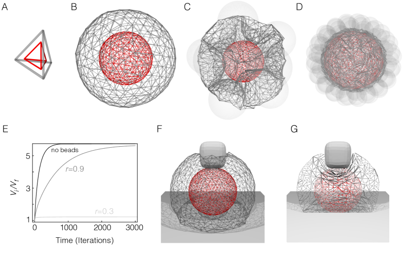
Figure 3: Modeling swelling hydrogels under confinement using tetrahedral meshes and level-set constraints. In all sections, red colored mesh elements represent the initial state whereas the dark gray colored elements represent the final state. While the meshes are full 3D, only line elements at the boundary are displayed here for simplicity. Confinements / obstacles are shown in light gray. A A representative tetrahedral element, which forms the basis of the 3D Morpho meshes, before and after swelling. B A swollen spherical hydrogel without any constraints. C, D Hydrogel swelling in the presence of stationary hard sphere beads. E Relative change in volume as a function of time, under equal step-size gradient descent dynamics, for the unconstrained swelling in B and the constrained swelling in C and D. F Swelling in the proximity of a stationary impenetrable plane and a superellipsoid. G Planar slice of the mesh in F showing expansion around the superellipsoid.

Hydrogels comprise two components, a polymer network infiltrated by water. By adjusting the crosslinking density, fill fraction, etc. the rigidity of the gel can be adjusted across many orders of magnitude. Furthermore, these materials have an incredible capacity to absorb water while remaining intact [42] making them amenable to a variety of different practical applications [43]. Due to the inevitable shape change that occurs, continuum modeling of hydrogels is often restricted to simple geometries. Incorporating constraints presents further challenges [44]. Here, we model a 3D hydrogel using a tetrahedral mesh. We adopt the Flory-Rehner formalism [45], wherein the free energy $F$ is the sum of a mixing term and an entropic elastic term. We ignore the ionic contribution for now, but this can be easily incorporated. Equilibrium is defined by the balance of osmotic pressures, $\partial F/\partial N_{\text{s}}=0$, with $N_{\text{s}}$ being the number of solvent molecules. We equivalently write the free energy in terms of the volume fraction of the polymer $\phi$, which makes it easier to connect to other formalisms for the energy [46]. We can compute this energy for any tetrahedron in the mesh, given its initial values for the volume $V_{\text{i}}$ and volume fraction $\phi_{\text{i}}$ together with a reference volume fraction $\phi_{0}$ [45]. The resulting total energy is then minimized (see Methods) to obtain the equilibrium shape and size of the hydrogel.

Figure 3A shows a representative tetrahedral element used in the computation. The finite-element approach allows us to realize arbitrary initial shapes of the hydrogel using a tetrahedral mesh. Here, we begin with a spherical mesh, where the result is a spherical shape of different size. The parameters of the Flory-Rehner functional determine the equilibrium volume fraction $\phi_{\text{eq}}$, and correspondingly, the expected change in volume $V_{\text{eq}}/V_{\text{i}}$. Setting this ratio to be $\approx 6$, we perform gradient descent to reach the equilibrium. Figure 3B shows the initial mesh in red and the final mesh in gray.

Morpho provides a convenient type of constraint, whereby vertices can be excluded from a region defined by the contours or level-sets of a scalar function. Using this, we can easily add confinement to the model computation. Inspired by recent beautiful experimental measurements [47], we introduce hard sphere beads surrounding the hydrogel. Figure 3C shows the resulting swollen hydrogel. In Figure 3D, we plot the ratio of the current volume to the initial volume for the case of unconfined and confined hydrogels from B and C, respectively. We can see a decrease in the swelling comparable to what is observed in [47]. To demonstrate the flexibility in the constraint application, Figure 3E and F show, respectively, the full 3D and a cross section of the swollen hydrogel in the presence of non-trivial confinements like a hard wall and a super-ellipsoidal bead together.

Lastly, such a simulation allows access to quantities that are harder to probe via experiments, such as the local strain during swelling, or the trend across varying material parameters. The programmable environment of Morpho allows for such an analysis directly without the need for external tools.

II Discussion

In this Article, we presented Morpho, a programmable environment that aims to solve a broad class of shape optimization and shape-shifting problems. Using an explicit method as used in software such as the Surface Evolver, we provide a programmable environment that goes beyond minimal surfaces and allows for domains and fields to be minimized together in arbitrary number of dimensions. Morpho provides additional features to facilitate mesh quality control: Leveraging the fact that shape optimization problems are often underdetermined, e.g. that the vertex positions for a minimal surface are uniquely specified only up to local tangential displacements, we employ auxiliary functionals that regularize the mesh elements and avoid clustering of vertices during optimization.

We demonstrated Morpho’s applicability to a variety of domains through three examples: In the first, minimizing the area of a closed membrane given a fixed volume, regularization permits the program to converge on the correct solution and improves the speed of convergence while the unregularized problem fails to converge.

In a second example, we showed the combined minimization of the shape as well as associated fields in liquid crystal tactoids. The customizable environment of Morpho allows for automated adaptive refinement based on heuristics (or error estimators if available) such as energy density, enabling us to resolve liquid crystal defects known as boojums that occur in some tactoid solutions. We further demonstrated the solution of a multiphysics problem where we found shapes of tactoids elongated in the presence of an electric field, solving for the shape, liquid crystal director as well as the electric field.

Our final example showed constrained optimization by simulating hydrogels swelling under arbitrary confinement as well as Morpho’s visualization capabilities, such as 3D ray-tracing provided by the povray module and the 2D slice visualization made possible by the meshslice module.

Beyond these examples, Morpho could be used for many other domains of science and engineering, including wetting problems, liquid crystal membranes, thin shell problems, and so on. It could also be used for purely mathematical purposes such as computing arbitrary minimal surfaces like a 3-periodic gyroid and its variants.

While the program as initially released is capable of solving a wide class of problems, we aim to further broaden the scope of Morpho by developing a number of improvements. We plan to expand the range of discretizations available for both shape and fields, and incorporate improved optimization algorithms. Applications beyond optimization, e.g. non-equilibrium dynamics as is central to active biological materials [18, 19], will be an important future target.

Morpho is entirely open-source under an MIT license and is provided with thorough documentation, readable from within the program in interactive mode or through a website as well as an extensive user manual. Morpho is built with an automated testing suite to facilitate a high degree of reliability. While the program is already competitive with other software used in this space, we are presently working on GPU acceleration to further improve performance. We hope that the availability of our robust, well-tested open-source shape optimization software will benefit the soft matter physics community in particular and researchers interested in shape optimization and shape shiftin problems at large.

III Methods

In the following subsections, we use boldface type to indicate classes of object, italic type to refer to modules available within Morpho and typewriter font to refer to external programs.

III.1 Morpho overview

III.1.1 Model

Morpho’s organizing metaphor for shape optimization involves the following classes of object:

Meshes may incorporate elements of various types. Meshes are graded, i.e., can incorporate point-like, line-like, area-like elements, etc. that are stored separately. Each element is associated with an integer id value. Connectivity information is stored in sparse matrices to facilitate use of efficient graph algorithms. To specify a mesh, it is only necessary to specify which vertices correspond to each element; additional connectivity information is automatically generated as needed.

Fields are object collections that store floating point information, i.e., scalars or matrices, on elements of a mesh. A field may assign any number of quantities to each element, and may store a different number of quantities on elements of each grade. To facilitate fast operations, the underlying data store is monolithic and arithmetic operations implemented via BLAS etc.

Functional objects correspond to terms in the energy functional and facilitate summation of contributions from individual elements. Given a mesh and any required fields, a Functional can return the total value corresponding to summing over elements in the mesh, a matrix of values for each element, the forces on each vertex and generalized forces on Field degrees of freedom.

Selections are objects that represent selected portions of a mesh. Each element can be selected or not. Selection objects can then be used to achieve various effects, such as restricting a functional to a particular subset of the mesh, or displaying a region of interest.

III.1.2 Scripting language

Morpho provides a simple but powerful object-oriented scripting language to describe and solve optimization problems. The syntax resembles other languages in the C family but has been kept small and clean to facilitate a low barrier to entry, inspired by the Lox language[48]. Despite its simplicity, the language provides very good performance and supports many features expected in a modern dynamic language: modules, classes, closures and many common collection types such as lists, dictionaries and matrices both dense and sparse. Linear algebra utilizes efficient libraries such as BLAS[49], LAPACK[50] and SuiteSparse[51]. The environment is highly extendable; a number of modules (all written in the Morpho language) are included as standard and implement important Morpho functionality. The user can easily add to these as they wish. The environment also provides good performance: scripts are compiled to an efficient bytecode for fast execution by a virtual machine, and the interpreter is among the fastest available.

III.1.3 Optimization

Optimization is provided by a separate optimize module. The problem to be solved—the target functional—is described by creating an OptimizationProblem object followed by creating and adding Functional objects. For example, the problem,

$$\text{Minimize}\ {\sigma\int_{\partial C}dA}+{\kappa\int_{\partial C}H^{2}dA}\ \text{s.t.}\ {\int_{C}dV}=V_{0},$$

is represented in Morpho through an Area object, a MeanCurvatureSq object and a VolumeEnclosed object. The first two terms are added to the OptimizationProblem using the addenergy method (with appropriate prefactors) and hence form part of the objective function to be minimized. The volume constraint is added to the problem using the addconstraint method. Target values for constraints may be specified, otherwise they are deduced from the initial state of the system.

Optimization is achieved by using ShapeOptimizer and FieldOptimizer objects which act on a given OptimizationProblem. Optimizer objects invoke the appropriate methods on each functional to calculate the current total value of the target functional for the given configuration as well as its gradient with respect to vertex positions or field degrees of freedom.

As a simple illustrative example, consider a single triangular element with vertices $\mathbf{x}_{0}$, $\mathbf{x}_{1}$ and $\mathbf{x}_{2}$. The area of the element is given by,

$$A=\frac{1}{2}\left|(\mathbf{x}_{1}-\mathbf{x}_{0})\times(\mathbf{x}_{2}-\mathbf{x}_{1})\right|,$$

from which we can readily compute $\nabla_{\mathbf{x}_{i}}A$, the gradient with respect to each vertex position. Suppose all vertex positions are stored sequentially in a single column vector $\mathbf{x}$; then we may similarly define a gradient column vector $\mathbf{g}=\nabla A$ from the set of gradients with respect to individual positions, $\nabla_{\mathbf{x}_{i}}A,\forall i\in\{0,1,2\}$. For a mesh consisting of many triangles, we can compute the total area and the gradient of the area with respect to each vertex position by summing up the contributions from each element. Each Functional object provides methods total and gradient to return exactly these objects.

ShapeOptimizer and FieldOptimizer provide a number of standard algorithms for optimization[52], including gradient descent, where the vertex positions are updated,

$$\mathbf{x}_{i+1}=\mathbf{x}_{i}-\alpha\mathbf{g}_{i},$$

for a fixed learning rate $\alpha$ and gradient of the target functional $\mathbf{g}_{i}$. Also available are backtracking linesearches and conjugate gradient methods for unconstrained optimization, with others forthcoming. Constraints are handled via a projection method as follows. First, the gradient of the constraint functional $\mathbf{h}_{i}$ is computed as for the target functional. The descent direction is then computed by projecting out the component of $\mathbf{g}_{i}$ in the direction of $\mathbf{h}_{i}$,

$$\mathbf{p}_{i}=\mathbf{g}_{i}-\frac{\mathbf{g}_{i}\cdot\mathbf{h}_{i}}{\mathbf{h}_{i}\cdot\mathbf{h}_{i}}\mathbf{h}_{i}.$$

Optimization proceeds using the descent direction $\mathbf{p}_{i}$ in place of the gradient. Following each iteration, re-projection steps are then taken to re-satisfy the constraint. A tolerance may be set to control the fidelity with which the constraint is maintained. A number of possible convergence criteria may be set, including convergence of the energy, the norm of the change in the position of the vertices, etc.

III.1.4 Visualization and data interchange

Simple but powerful support for visualization is provided by two modules. The plot module enables the user to conveniently visualize meshes, fields and selections. This uses the low-level module, graphics, that represents a scene as a list of 3D graphics primitives, including spheres, cylinders, tubes, arrows, collections of simplices and text. The abstract representation empowers the user to easily create custom visualizations, and enables output to different formats.

One such target is an included viewer application, morphoview, that is provided for convenient viewing. A further module, povray, integrates with the widely used povray raytracer [53] to convert graphics objects to give easy access to raytraced output: All figures in this manuscript were generated by Morpho and rendered with povray.

More sophisticated visualizations can be produced using external applications like Paraview; to facilitate interchange with such programs Morpho can export meshes and data in the commonly used VTK format.

III.2 Application details

III.2.1 Minimal surfaces and membranes

To solve the minimal surface problem, we construct an initial ellipsoidal Mesh with aspect ratio $2$ by stretching an initially spherical mesh. The problem is then set up as follows: An OptimizationProblem object is defined with an Area object to compute the surface area, and an VolumeEnclosed object added as a constraint. Optimization is performed using a ShapeOptimizer object and successive linesearches are performed until the relative change in the energy is $<10^{-8}$.

To incorporate regularization, a secondary OptimizationProblem is created incorporating an EquiElement object and the VolumeEnclosed object added as a constraint. A second ShapeOptimizer object is used to perform the regularization. To perform optimization, we now interleave linesearches on the surface tension and regularization problems, finding that a ratio of around 2:1 leads to satisfactory convergence.

Visualization of the solutions is performed using the plot module. As shown in Fig. 1, without regularization the problem rapidly gets stuck as elements near the cap shrink due to clustering of the vertices.

The membrane problem is solved using an initial disk Mesh created with the meshgen module. An OptimizationProblem is created for the target problem including Area and MeanCurvatureSq functionals, as well as a secondary OptimizationProblem with an EquiElement object. During optimization, certain vertices near the center of the disk are held at a fixed height using a level set constraint imposed using a ScalarPotential object. Optimization is performed using ShapeOptimizer objects with the target and regularization regularization steps interleaved. Once convergence is achieved, the tethered vertices are moved to a new height and the shape re-optimized. Discrete refinement moves are also performed at each of these new heights, where the mesh is equiangulated and large triangles split into smaller triangles.

III.2.2 Liquid crystal tactoids

To simulate the structure of the tactoid in Morpho, we first construct an initially spherical Mesh corresponding to the unit ball $\left|\mathbf{x}\right|^{2}<1$ with Morpho’s meshgen module. We also create a Field object to represent the nematic director $\mathbf{n}$ with an initially uniform configuration and a Selection object corresponding to the boundary of the mesh.

An OptimizationProblem object is then defined in Morpho by creating and adding the following functional objects: a Nematic object provides nematic elasticity; an Area object is used to evaluate the surface area on the boundary; an AreaIntegral is used to evaluate the anchoring energy. For two dimensional tactoids, the anchoring energy must be replaced with an equivalent LineIntegral. The director length constraint is imposed using a NormSq object that calculates the norm-squared of every entry in the field; this is added to the problem as a local constraint on the field $\mathbf{n}$. Finally, a Volume object is used to evaluate the volume of the mesh and is added to the optimization problem as a global constraint.

Having set up the problem, separate FieldOptimizer and ShapeOptimizer objects are created to optimize the field and shape individually. We use both these objects to perform conjugate gradient steps on $\mathbf{n}$ and the mesh respectively. We empirically find that interleaving field and shape optimization steps, with $\approx 4\times$ more field optimization steps, leads to reasonable convergence for the parameters considered. An energy convergence criterion is used whereby the optimization problem is considered to have converged when the relative change in the energy is $<10^{-8}$. Having obtained a coarse solution, we perform adaptive refinement by splitting elements with elastic energy $>1.5\times$ the mean using a MeshRefiner object from the meshtools module. We then optimize the refined solution as before.

Visualization of the solutions obtained is performed with the plot module. We write a custom function to represent the nematic configuration as a cylinder at every vertex and combine this with the surface of the tactoid visualized with the plot module; the combined output is then rendered using the povray module.

III.2.3 Swelling hydrogels

We use a thermodynamic theory of swelling hydrogels [54, 45, 55, 56]. Here, a binary polymer-solvent mixture is considered, with $N_{\text{p}}$ and $N_{\text{s}}$ being the number of polymer and solvent molecules respectively and $\nu_{\text{p}}$ and $\nu_{\text{s}}$ being the corresponding molar volumes. Equilibrium is reached when the chemical potential of the solvent is balanced inside and outside the hydrogel. Equivalently, this can be seen as minimizing the change in Helmholtz free energy $\Delta F$ with respect to the number of solvent molecules $N_{\text{s}}$. This change in the free energy, under a separability approximation, can we written as

$$\Delta F=\Delta F_{\text{mix}}+\Delta F_{\text{el}}.$$ (5)

The first term is the Flory-Huggins mixing contribution :

$$\Delta F_{\text{mix}}=N_{\text{s}}k_{\text{B}}T\left[\ln(1-\phi)+\chi\phi\right].$$ (6)

Here, $\phi$ is the volume fraction of the hydrogel, $\chi$ the Flory-Huggins mixing parameter, $k_{\text{B}}$ the Boltzmann constant and $T$ the temperature. Now, the osmotic pressure contribution from this energy is

$$\Pi_{\text{mix}}=-\frac{N_{\text{A}}}{\nu_{\text{s}}}\partialderivative{\Delta F_{\text{mix}}}{N_{\text{s}}},$$ (7)

with $N_{\text{A}}$ being Avogadro’s number. Note that $\phi$ is dependent on $N_{\text{s}}$:

$$\phi=\frac{N_{\text{p}}\nu_{\text{p}}}{(N_{\text{p}}\nu_{\text{p}}+N_{\text{s}}\nu_{\text{s}})}.$$ (8)

Using this relation, we can recover the osmotic pressure

$$\Pi_{\text{mix}}=-\frac{N_{\text{A}}}{\nu_{\text{s}}}\partialderivative{\Delta F_{\text{mix}}}{N_{\text{s}}}=-\frac{N_{\text{A}}k_{\text{B}}T}{\nu_{\text{s}}}\left[\phi+\ln(1-\phi)+\chi\phi^{2}\right].$$ (9)

Note that in the literature, this osmotic pressure is sometimes expressed in terms of an ‘effective diameter’ $\alpha$ of the solvent molecule [47]:

$$\Pi_{\text{mix}}=-\frac{k_{\text{B}}T}{\alpha^{3}}\left[\phi+\ln(1-\phi)+\chi\phi^{2}\right],$$ (10)

which implies $\alpha^{3}=\nu_{\text{s}}/N_{\text{A}}$.

The elastic contribution to the free energy, $\Delta F_{\text{el}}$, is given by the Flory-Rehner elastic energy [45, 55, 56],

$$\Delta F_{\text{el}}=-\frac{3N_{\text{c}}k_{\text{B}}T}{2}(\ln\beta-\beta^{2}+1),$$ (11)

where $N_{\text{c}}$ is the number of chains in the network and $\beta=(V/V_{0})^{1/3}=(\phi_{0}/\phi)^{1/3}$, with $V_{0}$ and $\phi_{0}$ being the volume and volume fraction respectively in the ‘reference’ state [45].

In this work, we consider a 3D polymer hydrogel in a solvent bath at a fixed temperature $T$, where the volume fraction of the polymer can vary over space. Hence, we want to think about a free energy density $\Delta f_{\text{mix}}(\mathbf{x})$, in terms of a spatially varying field $\phi(\mathbf{x})$. If this space is discretized using tetrahedra, it is useful to consider the expression (6) for a single tetrahedral element. The energy density locally at a point $\mathbf{x}$ in the deformed frame of reference will be Eq. (6) evaluated at $\mathbf{x}$ divided by the volume of the element. Since this volume would also be given by $N_{\text{p}}\nu_{\text{p}}+N_{\text{s}}\nu_{\text{s}}$, we have

$$\Delta f_{\text{mix}} =\frac{N_{\text{s}}}{N_{\text{p}}\nu_{\text{p}}+N_{\text{s}}\nu_{\text{s}}}k_{\text{B}}T\left[\ln(1-\phi)+\chi\phi\right]$$ (12)

$$=\frac{(1-\phi)}{\nu_{\text{s}}}k_{\text{B}}T\left[\ln(1-\phi)+\chi\phi\right].$$ (13)

In terms of $\alpha$, this would be

$$\Delta f_{\text{mix}}=\frac{k_{\text{B}}T}{N_{\text{A}}\alpha^{3}}\left[(1-\phi)\ln(1-\phi)+\chi\phi(1-\phi)\right].$$ (14)

Similarly for the elastic energy, we can compute the free energy by dividing by the volume. In this work, we assume that the chains are uniformly distributed throughout the hydrogel, so $N_{\text{c}}$ doesn’t depend on $\mathbf{x}$, but the functionality in Morpho can be easily extended to allow a spatially varying initial $N_{\text{c}}$.

Finally, we note that it follows from Eq.(8) that minimizing w.r.t. $N_{\text{s}}$ is equivalent to minimizing w.r.t. $\phi$. We thus connect to an equivalent formalism [46] and implement the minimization w.r.t. $\phi$ in Morpho. It can be seen that we have three non-dimensional parameters, namely, the Flory-Huggins mixing parameter $\chi$, the relative strength of the elastic energy to the mixing energy $N_{\text{c}}\alpha^{3}/V_{0}$ and the reference volume fraction $\phi_{0}$ [45]. Given an initial value of $\phi$, we can vary these parameters to change the minima of the overall free energy, thus tuning the swelling ratio (since $\phi_{\text{final}}$ affects $V_{\text{final}}$).

To compute the structure of the hydrogel in Morpho, we again start by constructing an initially spherical Mesh corresponding to the unit ball $\left|\mathbf{x}\right|^{2}<1$ with morpho’s meshgen module. An OptimizationProblem object is then defined and a Hydrogel functional, implementing the above discussed free energy density, is added to it. For hard confinements, we define level-set constraints corresponding to the objects (spheres, ellipsoids, planes, etc.) through the ScalarPotential object from the functionals module. A ShapeOptimizer object is then created to optimize the shape. We perform gradient descent with a fixed step size to simulate inviscid dynamics of the swelling. A Volume object is used to keep track of the volume of the hydrogel during relaxation.

To initialize the positions of the hard spheres for Figure 3C, we define a dummy shell mesh with radius $R+R_{\text{bead}}$ with $N_{\text{bead}}$ number of vertices placed randomly. We first confine the vertices to lie on the shell by using a ScalarPotential object. We then define an electrostatic repulsive pairwise interaction between the vertices using a PairwisePotential object from the functionals module, thus proceeding to solve the Thomson problem. The resulting mesh vertex positions are used as the sphere centers for the level set constraints. We thus get equidistantly packed spheres on the outer shell.

All 3D visualizations in Figure 3 are made using the povray module. The superellipsoid constraint in 3E and 3F is shown by constructing an equivalent mesh using the meshgen module and plotting its facets. Similarly, the plane is plotted by defining an equivalent planar mesh, while the slice in 3F is plotted using the meshslice module.

Data availability

Source data are provided with this paper.

Code availability

The Morpho application can be found at https://github.com/Morpho-lang/morpho. A manual is included in the repository, together with a number of examples. Source code for all examples shown in this publication can be found at https://github.com/Morpho-lang/morpho-paper. All code is released under an open source MIT License.

References

- Wehner et al. [2016] M. Wehner, R. L. Truby, D. J. Fitzgerald, B. Mosadegh, G. M. Whitesides, J. A. Lewis, and R. J. Wood, An integrated design and fabrication strategy for entirely soft, autonomous robots, Nature 536, 451 (2016).
- Booth et al. [2018] J. W. Booth, D. Shah, J. C. Case, E. L. White, M. C. Yuen, O. Cyr-Choiniere, and R. Kramer-Bottiglio, OmniSkins: Robotic skins that turn inanimate objects into multifunctional robots, Science Robotics 3, eaat1853 (2018).
- da Cunha et al. [2020] M. P. da Cunha, M. G. Debije, and A. P. H. J. Schenning, Bioinspired light-driven soft robots based on liquid crystal polymers, Chemical Society Reviews 49, 6568 (2020).
- Shah et al. [2021] D. S. Shah, J. P. Powers, L. G. Tilton, S. Kriegman, J. Bongard, and R. Kramer-Bottiglio, A soft robot that adapts to environments through shape change, Nature Machine Intelligence 3, 51 (2021).
- Mengaldo et al. [2022] G. Mengaldo, F. Renda, S. L. Brunton, M. Bächer, M. Calisti, C. Duriez, G. S. Chirikjian, and C. Laschi, A concise guide to modelling the physics of embodied intelligence in soft robotics, Nature Reviews Physics , 1 (2022).
- Kaplan et al. [2010] C. N. Kaplan, H. Tu, R. A. Pelcovits, and R. B. Meyer, Theory of depletion-induced phase transition from chiral smectic- A twisted ribbons to semi-infinite flat membranes, Physical Review E 82, 021701 (2010).
- Xing et al. [2012] X. Xing, H. Shin, M. J. Bowick, Z. Yao, L. Jia, and M.-H. Li, Morphology of nematic and smectic vesicles, Proceedings of the National Academy of Sciences 109, 5202 (2012).
- Giomi [2012] L. Giomi, Hyperbolic Interfaces, Physical Review Letters 109, 136101 (2012).
- Gibaud et al. [2017] T. Gibaud, C. N. Kaplan, P. Sharma, M. J. Zakhary, A. Ward, R. Oldenbourg, R. B. Meyer, R. D. Kamien, T. R. Powers, and Z. Dogic, Achiral symmetry breaking and positive Gaussian modulus lead to scalloped colloidal membranes, Proceedings of the National Academy of Sciences 114, 10.1073/pnas.1617043114 (2017).
- Ding et al. [2021] L. Ding, R. A. Pelcovits, and T. R. Powers, Deformation and orientational order of chiral membranes with free edges, Soft Matter 17, 6580 (2021).
- Carenza et al. [2022] L. N. Carenza, G. Gonnella, D. Marenduzzo, G. Negro, and E. Orlandini, Cholesteric Shells: Two-Dimensional Blue Fog and Finite Quasicrystals, Physical Review Letters 128, 027801 (2022).
- Khanra et al. [2022] A. Khanra, L. L. Jia, N. P. Mitchell, A. Balchunas, R. A. Pelcovits, T. R. Powers, Z. Dogic, and P. Sharma, Controlling the shape and topology of two-component colloidal membranes, Proceedings of the National Academy of Sciences 119, e2204453119 (2022).
- Safdari et al. [2021] M. Safdari, R. Zandi, and P. van der Schoot, Effect of electric fields on the director field and shape of nematic tactoids, Physical Review E 103, 062703 (2021).
- Silverberg et al. [2014] J. L. Silverberg, A. A. Evans, L. McLeod, R. C. Hayward, T. Hull, C. D. Santangelo, and I. Cohen, Using origami design principles to fold reprogrammable mechanical metamaterials, Science 345, 647 (2014).
- Silverberg et al. [2015] J. L. Silverberg, J.-H. Na, A. A. Evans, B. Liu, T. C. Hull, C. D. Santangelo, R. J. Lang, R. C. Hayward, and I. Cohen, Origami structures with a critical transition to bistability arising from hidden degrees of freedom, Nature Materials 14, 389 (2015).
- Paulose et al. [2015] J. Paulose, B. G.-g. Chen, and V. Vitelli, Topological modes bound to dislocations in mechanical metamaterials, Nature Physics 11, 153 (2015).
- Keber et al. [2014] F. C. Keber, E. Loiseau, T. Sanchez, S. J. DeCamp, L. Giomi, M. J. Bowick, M. C. Marchetti, Z. Dogic, and A. R. Bausch, Topology and dynamics of active nematic vesicles, Science 345, 1135 (2014).
- Giomi and Desimone [2014] L. Giomi and A. Desimone, Spontaneous division and motility in active nematic droplets, Physical Review Letters 112, 1 (2014).
- Maroudas-Sacks et al. [2020] Y. Maroudas-Sacks, L. Garion, L. Shani-Zerbib, A. Livshits, E. Braun, and K. Keren, Topological defects in the nematic order of actin fibers as organization centers of Hydra morphogenesis, Nature Physics 10.1101/2020.03.02.972539 (2020).
- Vutukuri et al. [2020] H. R. Vutukuri, M. Hoore, C. Abaurrea-Velasco, L. van Buren, A. Dutto, T. Auth, D. A. Fedosov, G. Gompper, and J. Vermant, Active particles induce large shape deformations in giant lipid vesicles, Nature 586, 52 (2020).
- Peterson et al. [2021] M. S. E. Peterson, A. Baskaran, and M. F. Hagan, Vesicle shape transformations driven by confined active filaments, Nature Communications 12, 7247 (2021).
- Khoromskaia and Salbreux [2021] D. Khoromskaia and G. Salbreux, Active morphogenesis of patterned epithelial shells, arXiv:2111.12820 [cond-mat, physics:physics, q-bio] (2021), arXiv:2111.12820 [cond-mat, physics:physics, q-bio] .
- Hoffmann et al. [2022] L. A. Hoffmann, L. N. Carenza, J. Eckert, and L. Giomi, Theory of defect-mediated morphogenesis, Science Advances 8, eabk2712 (2022).
- Jensen et al. [2015] K. E. Jensen, R. Sarfati, R. W. Style, R. Boltyanskiy, A. Chakrabarti, M. K. Chaudhury, and E. R. Dufresne, Wetting and phase separation in soft adhesion, Proceedings of the National Academy of Sciences 112, 14490 (2015).
- Datta et al. [2016] S. S. Datta, A. Preska Steinberg, and R. F. Ismagilov, Polymers in the gut compress the colonic mucus hydrogel, Proceedings of the National Academy of Sciences 113, 7041 (2016).
- Sydney Gladman et al. [2016] A. Sydney Gladman, E. A. Matsumoto, R. G. Nuzzo, L. Mahadevan, and J. A. Lewis, Biomimetic 4D printing, Nature Materials 15, 413 (2016).
- Na et al. [2015] J.-H. Na, A. A. Evans, J. Bae, M. C. Chiappelli, C. D. Santangelo, R. J. Lang, T. C. Hull, and R. C. Hayward, Programming Reversibly Self-Folding Origami with Micropatterned Photo-Crosslinkable Polymer Trilayers, Advanced Materials 27, 79 (2015).
- Goodman-Strauss and Sullivan [2003] C. Goodman-Strauss and J. M. Sullivan, Cubic polyhedra, in Discrete geometry (Marcel Dekker, 2003).
- Hawkes et al. [2010] E. Hawkes, B. An, N. M. Benbernou, H. Tanaka, S. Kim, E. D. Demaine, D. Rus, and R. J. Wood, Programmable matter by folding, Proceedings of the National Academy of Sciences 107, 12441 (2010).
- Provatas and Elder [2010] N. Provatas and K. Elder, Phase-field methods in materials science and engineering (Wiley-VCH, 2010).
- Chen [2002] L.-Q. Chen, Phase-Field Models for Microstructure Evolution, Annual Review of Materials Research 32, 113 (2002).
- Sethian [2010] J. A. Sethian, Level set methods and fast marching methods: Evolving interfaces in computational geometry, Fluid Mechanics, computer vision, and Materials Sciences (Cambridge Univ. Press, 2010).
- Brakke [1992] K. A. Brakke, The surface evolver, Experimental Mathematics 1, 141 (1992), https://doi.org/10.1080/10586458.1992.10504253 .
- Brakke et al. [1996] K. A. Brakke, J. Klinowski, and A. L. Mackay, The Surface Evolver and the stability of liquid surfaces, Philosophical Transactions of the Royal Society of London. Series A: Mathematical, Physical and Engineering Sciences 354, 2143 (1996).
- Canham [1970] P. B. Canham, The minimum energy of bending as a possible explanation of the biconcave shape of the human red blood cell, Journal of Theoretical Biology 26, 61 (1970).
- Helfrich [ Dec] W. Helfrich, Elastic properties of lipid bilayers: Theory and possible experiments, Zeitschrift Fur Naturforschung. Teil C: Biochemie, Biophysik, Biologie, Virologie 28, 693 (1973 Nov-Dec).
- Kamien [2002] R. D. Kamien, The geometry of soft materials: A primer, Reviews of Modern Physics 74, 953 (2002).
- Powers et al. [2002] T. R. Powers, G. Huber, and R. E. Goldstein, Fluid-membrane tethers: minimal surfaces and elastic boundary layers, Physical Review E 65, 041901 (2002).
- de and Prost [1993] G. P. G. de and J. Prost, The physics of liquid crystals (Clarendon Press, 1993).
- Prinsen and van der Schoot [2003] P. Prinsen and P. van der Schoot, Shape and director-field transformation of tactoids, Physical Review E 68, 021701 (2003).
- Mottram and Newton [2014] N. J. Mottram and C. J. P. Newton, Introduction to Q-tensor theory, arXiv:1409.3542 [cond-mat] (2014), arXiv:1409.3542 [cond-mat] .
- Bertrand et al. [2016] T. Bertrand, J. Peixinho, S. Mukhopadhyay, and C. W. MacMinn, Dynamics of Swelling and Drying in a Spherical Gel, Physical Review Applied 6, 064010 (2016).
- Ahmed [2015] E. M. Ahmed, Hydrogel: Preparation, characterization, and applications: A review, Journal of Advanced Research 6, 105 (2015).
- Kang and Huang [2010] M. K. Kang and R. Huang, A Variational Approach and Finite Element Implementation for Swelling of Polymeric Hydrogels Under Geometric Constraints, Journal of Applied Mechanics 77, 061004 (2010).
- Quesada-Pérez et al. [2011] M. Quesada-Pérez, J. A. Maroto-Centeno, J. Forcada, and R. Hidalgo-Alvarez, Gel swelling theories: The classical formalism and recent approaches, Soft Matter 7, 10536 (2011).
- Rognes et al. [2009] M. E. Rognes, M.-C. Calderer, and C. A. Micek, Modelling of and Mixed Finite Element Methods for Gels in Biomedical Applications, SIAM Journal on Applied Mathematics 70, 1305 (2009).
- Louf et al. [2021] J.-F. Louf, N. B. Lu, M. G. O’Connell, H. J. Cho, and S. S. Datta, Under pressure: Hydrogel swelling in a granular medium, Science Advances 7, eabd2711 (2021).
- Nystrom [2021] R. Nystrom, Crafting interpreters (Genever Benning, 2021).
- Blackford et al. [2002] L. S. Blackford, A. Petitet, R. Pozo, K. Remington, R. C. Whaley, J. Demmel, J. Dongarra, I. Duff, S. Hammarling, G. Henry, et al., An updated set of basic linear algebra subprograms (blas), ACM Transactions on Mathematical Software 28, 135 (2002).
- Anderson et al. [1999] E. Anderson, Z. Bai, C. Bischof, S. Blackford, J. Demmel, J. Dongarra, J. Du Croz, A. Greenbaum, S. Hammarling, A. McKenney, and D. Sorensen, LAPACK Users’ Guide, 3rd ed. (Society for Industrial and Applied Mathematics, Philadelphia, PA, 1999).
- Davis [2006] T. A. Davis, Direct methods for sparse linear systems (SIAM, 2006).
- Boyd et al. [2004] S. Boyd, S. P. Boyd, and L. Vandenberghe, Convex optimization (Cambridge university press, 2004).
- Persistence of Vision Pty. Ltd. [2004] Persistence of Vision Pty. Ltd., Persistence of vision raytracer [computer software] retrieved from http://www.povray.org/ (2004).
- Fernandez-Nieves [2011] A. Fernandez-Nieves, Microgel suspensions: Fundamentals and Applications (Wiley-VCH, 2011).
- Flory and Rehner [1943a] P. J. Flory and J. Rehner, Statistical Mechanics of Cross-Linked Polymer Networks I. Rubberlike Elasticity, The Journal of Chemical Physics 11, 512 (1943a).
- Flory and Rehner [1943b] P. J. Flory and J. Rehner, Statistical Mechanics of Cross-Linked Polymer Networks II. Swelling, The Journal of Chemical Physics 11, 521 (1943b).
- Note [1] Note that this expression is valid in the assumption that the number of polymer repeat units is much larger than 1.