Photon-Emission Statistics induced by Electron Tunnelling in Plasmonic Nanojunctions

Abstract

We investigate the statistics of photons emitted by tunneling electrons in a single electronic level plasmonic nanojunction. We compute the waiting-time distribution of successive emitted photons $w(\tau)$. When the cavity damping rate $\kappa$ is larger than the electronic tunneling rate $\Gamma$, we show that in the photon-antibunching regime, $w(\tau)$ indicates that the average delay-time between two successive photon emission events is given by $1/\Gamma$. This is in contrast with the usually considered second-order correlation function of emitted photons, $g^{(2)}(\tau)$, which displays the single time scale $1/\kappa$. Our analysis shows a relevant example for which $w(\tau)$ gives independent information on the photon-emission statistics with respect to $g^{(2)}(\tau)$, leading to a physical insight on the problem. We discuss how this information can be extracted from experiments even in presence of a non-perfect photon detection yield.

The correlation functions of the electromagnetic field are known to contain a rich amount of information about the intrinsic quantum nature of the electromagnetic field, as well as of the sources at the origin of photon emission Glauber (1963). The second-order correlation function (SCF) of the electromagnetic field $g^{(2)}(\tau)$, is of particular interest to investigate the statistics of photons emitted by fluorescent atoms or molecules Reynaud (1983); Carmichael et al. (1989); Cohen-Tannoudji and Reynaud (1979). It was shown that for a single-photon source, $g^{(2)}(\tau)$ vanishes at short times, a phenomenon known as photon antibunching Reynaud (1983). In the case that the emitter is a single atom or a molecule, photon antibunching is interpreted as arising from the wave-packet projection assumption of quantum mechanics Carmichael et al. (1989); Cohen-Tannoudji and Reynaud (1979) : after the first single-photon is emitted, the atom is projected back to its ground state. The emission of the next single-photon will then necessitate a finite delay-time during which the atom will be excited again, a necessary condition for another spontaneous emission event to occur.

Photon antibunching which was revealed by measurements of $g^{(2)}(\tau)$ for fluorescent single-molecules deposited on surfaces Verberk and Orrit (2003); Basché et al. (1992); Huang et al. (2016), is now a cornerstone of molecular spectroscopy. More recently, the progress in nanotechnologies extended the use of this experimental tool to design a wealth of different single-photon sources made of electrically-driven scanning tunneling microscopes (STM)Zhang et al. (2017); Merino et al. (2015); Rosławska et al. (2020); Leon et al. (2020); Nian et al. (2020); Doppagne et al. (2020), quantum dots Schuler et al. (2020); Yuan et al. (2002); Mizuochi et al. (2012); Nothaft et al. (2012); Schuler et al. (2020); Yuan et al. (2002), nitrogen vacancy centers Mizuochi et al. (2012), single-molecules deposited in molecular crystals Nothaft et al. (2012), and plasmonic nanocavities Gupta et al. (2021); Luo et al. (2019). The crossover to antibunching in presence of dissipation has also been investigated theoretically for waveguide quantum electrodynamics systems coupled to single atoms Chen et al. (2016, 2017). While most of these works deal with the paradigmatic two-level system model to describe photon antibunching, recent experiments with STM on C₆₀ molecular films invoke a Coulomb-blockade mechanism resulting from tip-induced split-off single-level states Leon et al. (2020). The actual mechanism at the origin of light-emission in current-driven STM nanojunctions is however still not well understood and might be more complex. In such systems indeed, current injection is believed to excite the molecule to an electronic excited-state that further decays back to ground state by emitting a photon. Several mechanisms were proposed for describing this molecular excitation, including elastic tunneling of an electron and a hole from the metallic electrodes to the molecule Doppagne et al. (2017), inelastic tunneling of an electron across the junction at the origin of emission of a localized plasmon that is further absorbed by the molecule Doppagne et al. (2017, 2018), and a more complex energy-transfer mechanism in which the absorption and emission processes of the localized plasmon by the molecule interfere one with each other Imada et al. (2017). Recently, we theoretically predicted that upon proper tuning of the external gate and electrode potentials, a single electronic level was sufficient to generate electrically-driven single-photon emission Schaeverbeke et al. (2019). In the same publication we found that $g^{(2)}(\tau)$ relaxes exponentially towards unity on a time scale given by the photon damping-time of the cavity $1/\kappa$ Schaeverbeke et al. (2019) and not with the electronic tunneling-time $1/\Gamma$. This is surprising, since electronic tunneling is the main physical mechanism at the origin of photon emission in the plasmonic nanocavity. To our knowledge, in the emerging field of nanoplasmonics there is still no complete understanding of which timescale is actually controlling photon antibunching. This question is of great experimental relevance to unravel the nature of the light-emission mechanism in current-driven single-photon sources.

In this Letter, we investigate theoretically the statistics of photon emission Barsegov and Mukamel (2002a, b); Jakeman and Loudon (1991) in a single-level plasmonic nanojunction, going beyond $g^{(2)}(\tau)$. In particular, we show that the delay-time or waiting-time distribution (WTD) $w(\tau)$ between successive photon-emission events Nienhuis (1988); Vyas and Singh (2000), provides important complementary statistical information to characterize the photon-emission statistics. The necessity to carefully discriminate between $w(\tau)$ an $g^{(2)}(\tau)$ is known in molecular fluorescence spectroscopy Reynaud (1983); Verberk and Orrit (2003); Lounis et al. (2000). Indeed, standard ”start-stop” photon correlators actually measure directly the WTD and not $g^{(2)}(\tau)$ Reynaud (1983). The difference between both quantities is nevertheless small for measurement times smaller than the average delay-time between photon emission events and for weak photon-detection yields Reynaud (1983); Lounis et al. (2000). The relevance of studying both $w(\tau)$ an $g^{(2)}(\tau)$ was recently noticed and successfully applied to the investigation of the full counting statistics of electronic currents in molecular junctions Brandes (2008); Albert et al. (2011, 2012); Seoane Souto et al. (2015); Kurzmann et al. (2019); Stegmann et al. (2021), or of the statistics of photon emission in microwave cavities Brange et al. (2019). However, such is not the case for current-induced single-photon sources, for which most studies do not discriminate clearly between these two quantities. We show how the joint calculation of $g^{(2)}(\tau)$ and $w(\tau)$ enables to unveil the timescales involved in the photon-emission process, thus paving the way for using these complementary observables in order to investigate both theoretically and experimentally the various existing mechanisms predicting current-driven photon antibunching.

Figure 1: Representation of a current-driven STM plasmonic nanojunction. The molecule is shown as a single electronic level of energy $\tilde{\varepsilon}_{0}$. In presence of a bias-voltage $V$, electrons from the STM apex (L) or from the substrate (R) can tunnel to the electronic level, emitting a cavity plasmon of frequency $\omega_{c}$. The former decays with rate $\kappa$, and a photon is emitted (red wavy arrow) that is finally collected by a detector (in black) with detection-yield $\eta$. Inset: Scheme of the rate equation for the occupation probabilities $P_{(q,n)}(t)$ of the dot charge and cavity plasmonic states $(q,n)$. The dominant transition rates for the parameters of Fig. 2 are shown. Thick red (thin blue) lines correspond to the dominant cavity-damping (sub-dominant inelastic single-electron tunneling) processes.

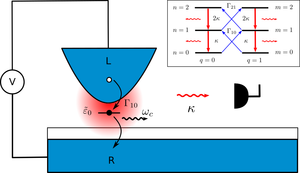
Stochastic model of photon-emission.—We consider the model of Ref. Schaeverbeke et al., 2019 describing a single electronic-level molecule embedded inside a STM nanojunction, and coupled to a cavity-plasmon mode (see Fig.1). The state of the plasmon-molecule subsystem is described by two indices $i\equiv(q,n)$ corresponding respectively to the charged (uncharged) dot-level $q=0(1)$, and occupancy state $n\in\mathbb{N}$ of the localized plasmon-mode (see inset of Fig.1). We consider the regime of sequential electronic tunneling and moderate cavity-damping $\Gamma\ll\kappa\leq k_{B}T/\hbar$ Schaeverbeke et al. (2019), with $T$ the temperature of the leads, $\hbar$ the reduced Planck constant and $k_{B}$ the Boltzmann constant. In this regime, the dynamics of the probability $P_{i}(t)$ of occupying the state $i$ is given by a rate-equation $\dot{P}_{i}(t)=\sum_{j}\Gamma_{ij}P_{j}(t)-\sum_{j}\Gamma_{ji}P_{i}(t)$, with $\Gamma_{ij}$ the incoherent rate for the transition $j\rightarrow i$. We consider two types of rates. The first one involves transitions which change the charge-state of the dot $(q,n)\rightarrow(\bar{q}=1-q,m)$ and modify by $m-n$ the occupancy of the cavity-plasmon mode. We associate to these transitions the corresponding inelastic tunneling rate of single-electrons across the junction: $\Gamma_{(\bar{q},m)(q,n)}=\sum_{\alpha}\Gamma_{\alpha}f_{q}\left(\Delta_{mn,\alpha}\right)|\left\langle n|\tilde{m}\right\rangle|^{2}$, with $\Gamma_{\alpha=L}$ the tunneling rate of electrons from the STM apex (L) lead to the dot, and $\Gamma_{\alpha=R}$ the tunneling rate from the substrate (R) lead to the dot. The factor $|\left\langle n|\tilde{m}\right\rangle|^{2}$ is the Franck-Condon overlap Koch et al. (2006) between the state $\left|n\right\rangle$ of the cavity with empty dot and the displaced-state $\left|\tilde{m}\right\rangle$ of the cavity with occupied dot. We introduced the functions $f_{q=0}\left(E\right)\equiv f(E)$ and $f_{q=1}\left(E\right)\equiv 1-f(E)$, with $f(E)=\left\{e^{E/k_{B}T}+1\right\}^{-1}$ the Fermi-Dirac distribution of the electrons populating the leads. This function is evaluated at the transition energy $\Delta_{mn,\alpha}=\tilde{\varepsilon}_{0}+\left(m-n\right)\hbar\omega_{c}-\mu_{\alpha}$, with $\tilde{\varepsilon}_{0}=\varepsilon_{0}-\lambda^{2}\hbar\omega_{c}$ the molecular dot-level energy renormalized by its coupling $\lambda$ to the cavity-mode expressed in units of $\hbar\omega_{c}$ Schaeverbeke et al. (2019), $\omega_{c}$ the cavity-plasmon frequency, and $\mu_{\alpha}$ the chemical potential of lead $\alpha$. The second type of rates involves transitions which do not change the charge state of the dot $(q,n)\rightarrow(q,n-1)$ and decrease by one the number of cavity-plasmons. Those incoherent transitions are associated to the cavity-photon losses $\Gamma_{(q,n-1)(q,n)}=\kappa n$, with $\kappa$ the cavity damping-rate at the origin of photon emission by the nanojunction.

Figure 2: Second-order correlation function $g^{(2)}(\tau)$ for the emitted photons as a function of time $\tau$, obtained numerically from the Monte Carlo simulations (averaged over 40 runs). Blue lower triangles are obtained for a plasmon-molecule coupling strength $\lambda=0.25$, cyan upper triangles for $\lambda=\sqrt{2-\sqrt{2}}\approx 0.77$ and red dots for $\lambda=\sqrt{2}\approx 1.41$. Plain curves are the analytical results from Eq. (6). Parameters are : $\eta=1$, $\kappa=k_{B}T/\hbar=0.1\omega_{c}$, $\Gamma_{L}=\Gamma_{R}=\Gamma=0.01\omega_{c}$, $\mu_{L}=-\mu_{R}=eV/2=\hbar\omega_{c}$, $\tilde{\varepsilon}_{0}=0$.

Monte Carlo approach.—We solve numerically the previous rate equation, using a kinetic Monte Carlo (MC) approach Fichthorn and Weinberg (1991); Gillespie (1976). We assign a probability, or detection yield, $\eta$ for each photon that has been emitted by the nanojunction to be finally collected and detected by an external photon detector, a perfect detection-yield meaning $\eta=1$. We suppose in the MC calculation that the photon-detection event by the photon detector is independent from the photon-emission event by the junction Sup . The output of the MC enables to record the history of random times at which a photon is emitted and detected. From those time-traces we extract $S(\tau)\equiv P\left(\tau|0\right)$ the conditional probability distribution that a photon is emitted and detected at time $\tau$, knowing that a photon has been emitted and detected at time $0$. Similarly, we obtain $Q\left(\tau|0\right)$, the probability distribution of the first-time photon detection event. It is defined as the exclusive conditional probability distribution of a photon emission and detection event at time $\tau$, knowing that the previous photon detection event occurred at time $0$, with the constraint that no other photon was emitted in the time interval $\left]0,\tau\right[$. The probability distributions $P$ and $Q$ are different, since the first one collects all possible photon emission and detection events in the intermediate time-interval $\left]0,\tau\right[$, while the second one excludes them all. The SCF and WTD of emitted and detected photons are obtained from those fundamental distributions as Sup

$$g^{(2)}(\tau) = \frac{S(\tau)}{\Gamma_{\gamma}^{(\rm{st})}}\,,$$ (1)

$$w(\tau) = Q\left(\tau|0\right)\,,$$ (2)

with $\Gamma_{\gamma}^{(\rm{st})}=\eta\kappa\left\langle n\right\rangle$ the rate or stationary probability per unit of time to emit and detect a photon, and $\left\langle n\right\rangle$ the average occupation of the cavity-plasmon mode.

Figure 3: Time-dependence of the distribution of delay-times $w(\tau)$ between two successive photon emission and detection events, obtained from the MC numerical calculation (yellow histogram), expressed in units of $\Gamma_{10}$. The blue plain (dashed red) curve is the outcome of the analytical formula in Eq. (10), for $\eta=0.75(1)$. Parameters are those of Fig. 2 with $\lambda=\sqrt{2}$, for which photon antibunching occurs.

Expressions for the SCF and WTD.—In the following, we write $P_{mn}^{q^{\prime}q}\left(\tau\right)$ the occupation probability of the plasmon-molecule state $(q^{\prime}m)$ at time $\tau$ that is solution of the rate equation, with the state $(qn)$ initially occupied. Similarly, we note $Q_{mn}^{q^{\prime}q}\left(\tau\right)$ the exclusive probability of first reaching the state $(q^{\prime}m)$, leading to a first-photon emission and detection event at time $\tau$, knowing that the state $(qn)$ was occupied at time $\tau=0$. From Eqs. (1) and (2), we derive the following expressions for the SCF and WTD (see Supplementary Material Sup for further details)

$$S(\tau) = \frac{\kappa\eta}{\left\langle n\right\rangle}\sum_{n,m=1}^{+\infty}\sum_{q,q^{\prime}=0,1}mnP_{mn-1}^{q^{\prime}q}\left(\tau\right)P^{(\rm{st})}_{(qn)}\,,$$ (3)

$$w(\tau) = \frac{\kappa\eta}{\left\langle n\right\rangle}\sum_{n,m=1}^{+\infty}\sum_{q,q^{\prime}=0,1}mnQ_{mn-1}^{q^{\prime}q}\left(\tau\right)P^{(\rm{st})}_{(qn)}\,,$$ (4)

with $P^{(\rm{st})}_{(qn)}=\lim_{\tau\rightarrow+\infty}P_{(qn)}\left(\tau\right)$ the stationary occupancy of the state $(qn)$. The $Q$-distribution is then solution of a renewal-like integral equation Carmichael et al. (1989)

$$P_{nm}^{qq^{\prime}}\left(\tau\right) = Q_{nm}^{qq^{\prime}}\left(\tau\right)+\kappa\sum_{k=1}^{+\infty}k\sum_{r=0,1}\left(P_{nk-1}^{qr}\ast Q_{km}^{rq^{\prime}}\right)\left(\tau\right)\,,$$

where we wrote $\left(g\ast h\right)\left(\tau\right)\equiv\int_{0}^{\tau}d\tau_{1}g\left(\tau-\tau_{1}\right)h\left(\tau_{1}\right)$ the convolution between any two causal functions $g$ and $h$. In general, Eq. (LABEL:RelationgPQ) has to be solved numerically, after Laplace transforming.

Figure 4: Average-delay time $\left\langle\tau\right\rangle$ in units of $\Gamma_{10}$ as a function of plasmon-molecule coupling $\lambda$, obtained from the MC numerical calculation. Upper orange (lower cyan) triangles correspond to the case of a perfect (non-perfect) detection yield $\eta=1(0.75)$. Red stars (blue dots) are the corresponding values of $1/\Gamma_{\gamma}^{(\rm{st})}\equiv 1/\eta\kappa\left\langle n\right\rangle$ appearing in Eq. (8). Dashed curves are the values of $\left\langle\tau\right\rangle$ given by approximate Eq. (12).

Results for the SCF.—In the rest of the paper, we consider the case of an electron-hole symmetric junction for which $\tilde{\epsilon}_{0}=0$, $\Gamma_{L}=\Gamma_{R}=\Gamma$, and $\mu_{L}=-\mu_{R}=eV/2$, with $V$ the bias-voltage between source and drain and $e$ the elementary charge. In this regime, the inelastic tunneling rates are independent of the charge state, namely $\Gamma_{(\bar{q},m)(q,n)}=\Gamma_{mn}$ for all $q=0,1$. The general case of asymmetric junctions regarding the SCF is considered in details in Ref. Schaeverbeke et al., 2019.

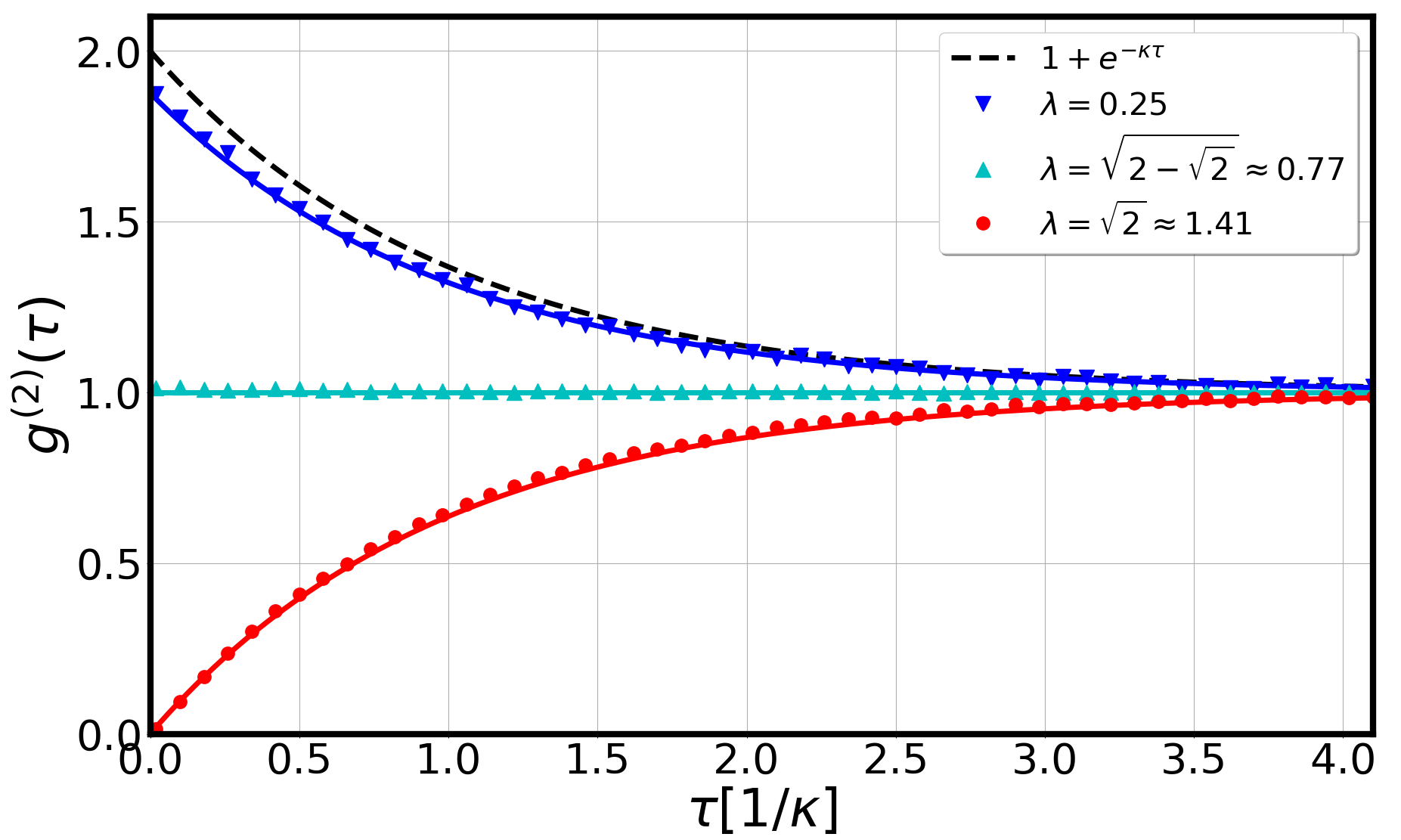
In Fig. 2, we show $g^{(2)}(\tau)$ as a function of time $\tau$, obtained from the MC simulations (averaged over 40 runs). The voltage-bias is fixed at the first inelastic threshold for photon-emission ($eV=2\hbar\omega_{c}$) and the photon detection is perfect ($\eta=1$). Upon increasing the plasmon-molecule coupling strength $\lambda$, we find a crossover in the SCF from photon-bunching to photon-antibunching. This result agrees with the results found in Ref. Schaeverbeke et al., 2019, derived with another method. In this range of parameters, the rate equation for $P_{(qn)}(t)$ is well approximated by truncating the available cavity-occupancies to $n\leq 2$ Schaeverbeke et al. (2019). The dominant transition rates are provided by the cavity-damping rate $\kappa$ (red downward arrows in inset of Fig. 1) and two single-electron inelastic tunneling rates $\Gamma_{10},\Gamma_{21}\ll\kappa$ (blue upward arrows). This truncated rate equation can be solved analytically exactly Sup , to provide in the regime $\kappa\gg\Gamma$

$$g^{(2)}(\tau) \approx 1+e^{-\kappa\tau}\left(g^{(2)}(0)-1\right)\,,$$ (6)

$$g^{(2)}(0) = \frac{\langle n(n-1)\rangle}{\langle n\rangle^{2}}\approx\frac{\Gamma_{21}}{\Gamma_{10}}=\frac{\left(2-\lambda^{2}\right)^{2}}{2}\,.$$ (7)

The analytical results of Eq. (6) are shown as plain curves in Fig. 2, and perfectly agree with the numerically exact MC. We thus confirm quantitatively the results of Ref. Schaeverbeke et al., 2019 that $g^{(2)}(\tau)$ relaxes exponentially in time towards unity, with a rate given by the cavity-damping rate $\kappa$. The convergence of $g^{(2)}(\tau)$ to $1$, is due to the fact that two distinct photon emission events separated by a time-interval $\tau\gg 1/\kappa$ become independent. The zero-delay behavior $g^{(2)}(0)$ between two emission events is given by Eq. (7). For weak plasmon-molecule coupling $\lambda=0.25<1$ (blue lower triangles), the stationary probability of having $n=2$ occupancy of the cavity-plasmon mode is significant. This results in an effective (out-of-equilibrium) thermal state characterized by photon bunching ($g^{(2)}(\tau)\leq g^{(2)}(0)=2$). For a critical value of $\lambda=\sqrt{2}$ (red points), the rate $\Gamma_{21}$ vanishes due to the vanishing of the Franck-Condon matrix element. This results in a vanishing probability to reach the $n=2$ occupancy, with only two possible occupations of the plasmon-mode $n=0,1$. This leads to $g^{(2)}(\tau)\geq g^{(2)}(0)=0$ and thus to photon antibunching, a fingerprint of single-photon emission. Finally the crossover region that is characterized by $g^{(2)}(\tau)=g^{(2)}(0)=1$ (Poissonian behavior), is reached for $\lambda=\sqrt{2-\sqrt{2}}$ (cyan upper triangles).

Results for the WTD.—We now consider the time-evolution of $w(\tau)$. The average delay-time between two successive photon emission and detection events $\left\langle\tau\right\rangle=\int_{0}^{+\infty}d\tau\tau w(\tau)$ can be derived analytically from Eqs. (4) and (LABEL:RelationgPQ), using a similar approach to the one used in computing polymer mean reaction times Guérin et al. (2012, 2013, 2013); Condamin et al. (2008). We obtain the general relation (see Sup for details)

$$\left\langle\tau\right\rangle = \frac{1}{\Gamma_{\gamma}^{(\rm{st})}}\equiv\frac{1}{\eta\kappa\left\langle n\right\rangle}\,,$$ (8)

which relates the average cavity-photon occupation $\left\langle n\right\rangle$ to the ratio between the dissipation-time $1/\kappa$ and the average delay-time $\left\langle\tau\right\rangle$. This relation is reminiscent of Kac’s lemma Kac (1947); Aldous and Fill (2002). It is expected to hold in any ergodic system, but as far as we know, Eq. (8) was not clearly identified before in the field of plasmonics.

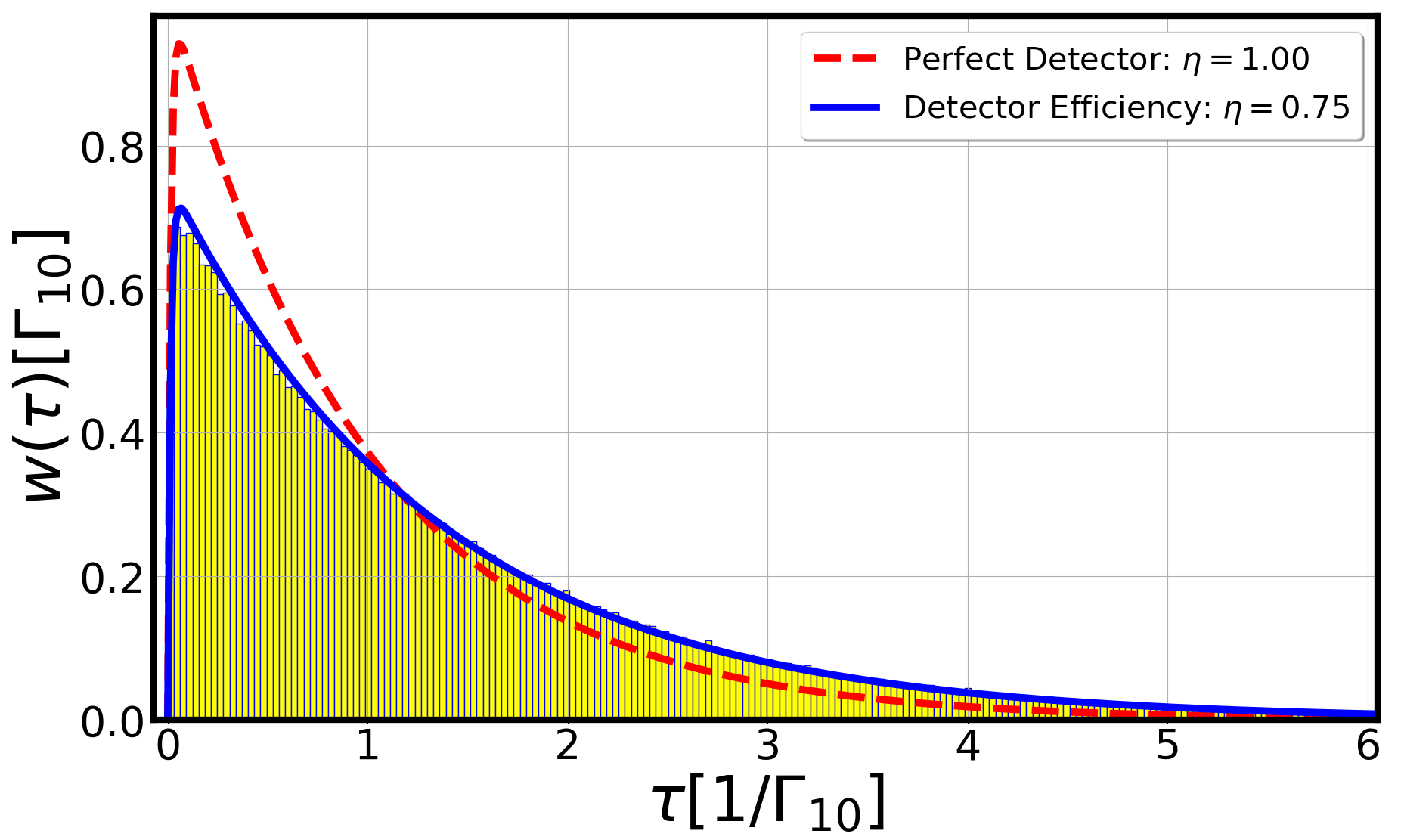
From now on, we focus on the case $\lambda=\sqrt{2}$, for which maximal antibunching occurs. We show in Fig. 3, the WTD computed numerically with the MC (yellow histogram), in the case of a non-perfect detection yield $\eta=0.75$. We obtain that $w(\tau)$ is a non-monotonous function of time, with a maximum at times $\tau\approx 1/\kappa$. In the same region of parameters for which Eq. (6) was derived, we obtain Sup

$$S(\tau) = \frac{\eta\kappa\Gamma_{10}}{\kappa_{t}}\left\{1-e^{-\kappa_{t}\tau}\right\}\,,$$ (9)

$$w(\tau) = \frac{\eta\kappa\Gamma_{10}}{\kappa_{d}}\left\{e^{-\frac{\left(\kappa_{t}-\kappa_{d}\right)\tau}{2}}-e^{-\frac{\left(\kappa_{t}+\kappa_{d}\right)\tau}{2}}\right\}\,,$$ (10)

with $\kappa_{d}=\sqrt{\kappa_{t}^{2}-4\eta\kappa\Gamma_{10}}$, and $\kappa_{t}=\kappa+\Gamma_{10}$.

Equation (10) is one of the main results of this paper. Its outcome is plotted as a plain(dashed) line in Fig. 3 for $\eta=0.75(1)$, and matches very well the MC histogram. At short delay-times ($\tau\ll 1/\kappa$), the antibunching mechanism implies that the probability of emitting two successive photons in a short delay-time $\tau$ is strongly reduced. The corresponding linear vanishing of $w(\tau)\approx\eta\kappa\Gamma_{10}\tau$ has a slope proportional to $\Gamma_{10}$. This is due to the fact that after the first emission event, inelastic tunneling of a single-electron across the nanojunction is necessary to emit another cavity-plasmon, that will later decay through a photon-emission event with rate $\kappa$. The slope also decreases with $\eta$, since it becomes less probable to detect the emitted photon upon worst detection-yield. At large delay-times ($\tau\gg 1/\kappa$), the WTD vanishes exponentially as $w(\tau)\approx\eta\Gamma_{10}e^{-\eta\Gamma_{10}\tau}$. This reflects the fact that a long time $\tau$ after the first emission event, it becomes very unlikely that another photon has not been emitted. At intermediate times ($\tau\approx 1/\kappa$), the maximum WTD is reached at a time $\tau_{m}$ such that

$$\tau_{m} = \frac{1}{\kappa_{d}}\ln\left(\frac{\kappa_{t}+\kappa_{d}}{\kappa_{t}-\kappa_{d}}\right)\approx\frac{1}{\kappa}\ln\left(\frac{\kappa}{\eta\Gamma_{10}}\right)\,.$$ (11)

The average delay-time $\left\langle\tau\right\rangle$ results from Eq. (10)

$$\left\langle\tau\right\rangle = \frac{1}{\eta}\left\{\frac{1}{\Gamma_{10}}+\frac{1}{\kappa}\right\}\,,$$ (12)

and recovers the result of Eq. (8), in the particular case $\lambda=\sqrt{2}$. The average delay-time $\left\langle\tau\right\rangle\approx 1/\eta\Gamma_{10}$ is thus proportional to the inelastic tunneling time of single-electrons across the junction $1/\Gamma_{10}$, corresponding to the necessary waiting-time needed for two successive current-driven photon-emission events to occur. As expected, the lower the detection-yield, the longer $\left\langle\tau\right\rangle$.

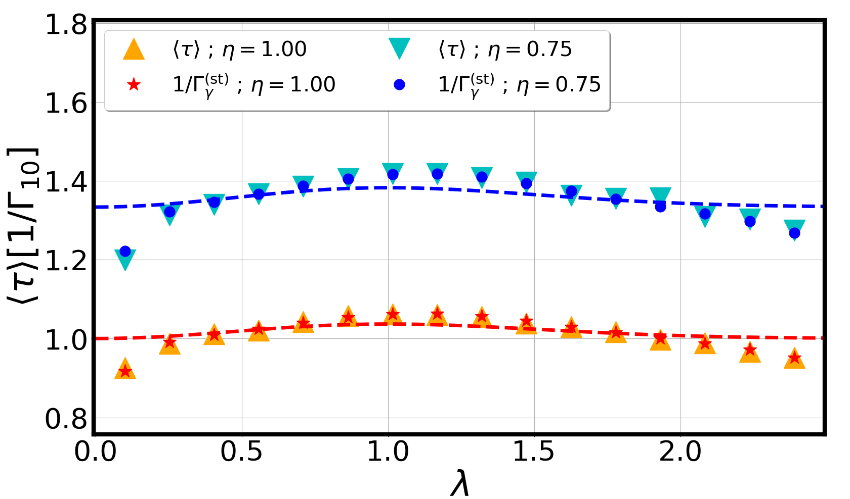
We show in Fig.4 the robustness of Eq. (8) away from the specific case $\lambda=\sqrt{2}$, for $\eta=0.75$ and $1$. The quantity $\left\langle\tau\right\rangle$ (lower cyan triangles) obtained from the MC, and $1/\Gamma_{\gamma}^{(\rm{st})}$ (blue dots) derived from solving for the stationary state in the rate equation, are shown to coincide as a function of $\lambda$, for $\eta=0.75$. The same good agreement is found for $\eta=1$. Surprisingly, in the range of moderate to strong plasmon-molecule coupling strengths ($\lambda\in\left[0.1,2.0\right]$), Eq. (12) is still a good approximation to the exact value of $\left\langle\tau\right\rangle$ (see blue dashed curve in Fig.4), despite a strong modulation of the rate $\Gamma_{10}$ with $\lambda$.

Furthermore, we note that an integral equation exists relating $S(\tau)$ and $w(\tau)$ Sup ,

$$S(\tau) = w(\tau)+\left(S\ast w\right)(\tau)\,,$$ (13)

that is consistent with Eqs. (9)-(10). Equation (13) was derived previously in Refs. Reynaud, 1983; Basché et al., 1992 for describing the stochastic Markovian dynamics of fluorescent two-level atoms or molecules. In our case, however, this relation is valid only at electron-hole symmetric point for $eV=2\omega_{c}$ and $\lambda=\sqrt{2}$, for which only two cavity states $n=0,1$ matter. In general, for arbitrary values of external parameters, the validity of this relation is not granted anymore, and one resorts with either MC simulations, or with solving numerically the linear system of Eqs. (LABEL:RelationgPQ) to obtain the $Q$-distribution and the WTD in Eq. (4). Finally, we remark that Eqs. (6) and (12) resolve the timescale issue noticed in the introduction. In the regime $\Gamma\ll\kappa$, there is no contradiction having $g^{(2)}(\tau)$ relaxing exponentially with the cavity-damping time $1/\kappa$, while the average delay-time $\left\langle\tau\right\rangle$ is given by the inverse inelastic tunneling time $1/\Gamma_{10}$ of single-electrons across the nanojunction. This difference of timescales is due to the fact that the SCF and WTD do not provide the same information about the statistics of photon emission and detection, and should thus be seen as complementary statistical indicators.

Conclusions.—We have investigated in depth the time-dependence of the second-order correlation function $g^{(2)}(\tau)$ and waiting-time distribution $w(\tau)$ of photons emitted by a current-induced plasmonic nanojunction with a single electronic level. By using MC and analytical calculations, we have shown that the two quantities provide a complementary information about the statistics of emitted photons by the nanojunction. In the regime of photon-antibunching, and when $\kappa\gg\Gamma$, $g^{(2)}(\tau)$ relaxes in time towards unity with the cavity damping-time $1/\kappa$, while the average delay-time $\left\langle\tau\right\rangle$ between successive photon emission and detection events is proportional to the inelastic tunneling time of single-electrons across the nanojunction $1/\Gamma_{10}$. We hope that our paper will stimulate further experiments in current-driven STM plasmonic nanojunctions, for which, to the best of our knowledge, a comparative measurement of the WTD with respect to the SCF of the emitted photons is still lacking, but seems to be crucial to understand better the timescales and physical mechanism involved in the current-induced light-emission process.

We acknowledge fruitful discussions with Guillaume Schull, Benoit Douçot and Javier Aizpurua about the statistics of photon emission, and with Ludovic Jaubert about kinetic MC simulations. We also thank Thomas Guérin for pointing out Kac’s lemma in our interpretation of the average delay-time between two photon emission events. This work was supported by IDEX Bordeaux (No. ANR-10-IDEX-03-02) and Euskampus Transnational Common Laboratory QuantumChemPhys. R. A. acknowledges financial support by the French Agence Nationale de la Recherche project CERCa, ANR-18-CE30-0006. T. F. acknowledges financial support by the Spanish AEI (FIS2017-83780-P and PID2020-115406GB-I00) and the European Union’s Horizon 2020 (FET-Open project SPRING Grant No. 863098). F. P. acknowledges support from the French Agence Nationale de la Recherche (grant SINPHOCOM ANR-19-CE47-0012).

References

- Glauber (1963) R. J. Glauber, Phys. Rev. 130, 2529 (1963).
- Reynaud (1983) S. Reynaud, in Annales de physique, Vol. 8 (EDP Sciences, 1983) pp. 315–370.
- Carmichael et al. (1989) H. Carmichael, S. Singh, R. Vyas, and P. Rice, Phys. Rev. A. 39, 1200 (1989).
- Cohen-Tannoudji and Reynaud (1979) C. Cohen-Tannoudji and S. Reynaud, Phil. Trans. R. Soc. Lond. A 293, 223 (1979).
- Verberk and Orrit (2003) R. Verberk and M. Orrit, J. Chem. Phys. 119, 2214 (2003).
- Basché et al. (1992) T. Basché, W. E. Moerner, M. Orrit, and H. Talon, Phys. Rev. Lett. 69, 1516 (1992).
- Huang et al. (2016) C.-H. Huang, Y.-H. Wen, and Y.-W. Liu, Opt. Express 24, 4278 (2016).
- Zhang et al. (2017) L. Zhang, Y.-J. Yu, L.-G. Chen, Y. Luo, B. Yang, F.-F. Kong, G. Chen, Y. Zhang, Q. Zhang, Y. Luo, J.-L. Yang, Z.-C. Dong, and J. Hou, Nat. Commun. 8, 1 (2017).
- Merino et al. (2015) P. Merino, C. Große, A. Rosławska, K. Kuhnke, and K. Kern, Nat. Commun. 6, 1 (2015).
- Rosławska et al. (2020) A. Rosławska, C. L. Christopher, A. Grewal, P. Merino, K. Kuhnke, and K. Kern, ACS Nano 14, 6366 (2020).
- Leon et al. (2020) C. C. Leon, O. Gunnarsson, D. de Oteyza, A. Rosławska, P. Merino, A. Grewal, K. Kuhnke, and K. Kern, ACS Nano 14, 4216 (2020).
- Nian et al. (2020) L.-L. Nian, T. Wang, Z.-Q. Zhang, J.-S. Wang, and J.-T. Lü, J. Phys. Chem. Lett. 11, 8721 (2020).
- Doppagne et al. (2020) B. Doppagne, T. Neuman, R. Soria-Martinez, L. López, H. Bulou, M. Romeo, S. Berciaud, F. Scheurer, J. Aizpurua, and G. Schull, Nat. Nanotechnol. 15, 207 (2020).
- Schuler et al. (2020) B. Schuler, K. Cochrane, C. Kastl, E. Barnard, E. Wong, N. Borys, A. Schwartzberg, D. Ogletree, F. de Abajo, and A. Weber-Bargioni, Sci. Adv. 6 (2020), 10.1126/sciadv.abb5988.
- Yuan et al. (2002) Z. Yuan, B. E. Kardynal, R. M. Stevenson, A. J. Shields, C. J. Lobo, K. Cooper, N. S. Beattie, D. A. Ritchie, and M. Pepper, Science 295, 102 (2002).
- Mizuochi et al. (2012) N. Mizuochi, T. Makino, H. Kato, D. Takeuchi, M. Ogura, H. Okushi, M. Nothaft, P. Neumann, A. Gali, F. Jelezko, et al., Nat. Photon. 6, 299 (2012).
- Nothaft et al. (2012) M. Nothaft, S. Höhla, F. Jelezko, N. Frühauf, J. Pflaum, and J. Wrachtrup, Nat. Commun. 3, 1 (2012).
- Gupta et al. (2021) S. Gupta, O. Bitton, T. Neuman, R. Esteban, L. Chuntonov, J. Aizpurua, and G. Haran, Nat. Commun. 12, 1 (2021).
- Luo et al. (2019) Y. Luo, G. Chen, Y. Zhang, L. Zhang, Y. Yu, F. Kong, X. Tian, Y. Zhang, C. Shan, Y. Luo, J. Yang, V. Sandoghdar, Z. Dong, and J. G. Hou, Phys. Rev. Lett. 122, 233901 (2019).
- Chen et al. (2016) Z. Chen, Y. Zhou, and J.-T. Shen, Opt. Lett. 41, 3313 (2016).
- Chen et al. (2017) Z. Chen, Y. Zhou, and J.-T. Shen, Phys. Rev. A 96, 053805 (2017).
- Doppagne et al. (2017) B. Doppagne, M. C. Chong, E. Lorchat, S. Berciaud, M. Romeo, H. Bulou, A. Boeglin, F. Scheurer, and G. Schull, Phys. Rev. Lett. 118, 127401 (2017).
- Doppagne et al. (2018) B. Doppagne, M. C. Chong, H. Bulou, A. Boeglin, F. Scheurer, and G. Schull, Science 361, 251 (2018).
- Imada et al. (2017) H. Imada, K. Miwa, M. Imai-Imada, S. Kawahara, K. Kimura, and Y. Kim, Phys. Rev. Lett. 119, 013901 (2017).
- Schaeverbeke et al. (2019) Q. Schaeverbeke, R. Avriller, T. Frederiksen, and F. Pistolesi, Phys. Rev. Lett. 123, 246601 (2019).
- Barsegov and Mukamel (2002a) V. Barsegov and S. Mukamel, J. Chem. Phys. 116, 9802 (2002a).
- Barsegov and Mukamel (2002b) V. Barsegov and S. Mukamel, J. Chem. Phys. 117, 9465 (2002b).
- Jakeman and Loudon (1991) E. Jakeman and R. Loudon, J. Phys. A: Math. Gen. 24, 5339 (1991).
- Nienhuis (1988) G. Nienhuis, J. Stat. Phys. 53, 417 (1988).
- Vyas and Singh (2000) R. Vyas and S. Singh, J. Opt. Soc. Am. B 17, 634 (2000).
- Lounis et al. (2000) B. Lounis, H. Bechtel, D. Gerion, P. Alivisatos, and W. Moerner, Chem. Phys. Lett. 329, 399 (2000).
- Brandes (2008) T. Brandes, Annalen der Physik 17, 477 (2008).
- Albert et al. (2011) M. Albert, C. Flindt, and M. Büttiker, Phys. Rev. Lett. 107, 086805 (2011).
- Albert et al. (2012) M. Albert, G. Haack, C. Flindt, and M. Büttiker, Phys. Rev. Lett. 108, 186806 (2012).
- Seoane Souto et al. (2015) R. Seoane Souto, R. Avriller, R. C. Monreal, A. Martín-Rodero, and A. Levy Yeyati, Phys. Rev. B 92, 125435 (2015).
- Kurzmann et al. (2019) A. Kurzmann, P. Stegmann, J. Kerski, R. Schott, A. Ludwig, A. D. Wieck, J. König, A. Lorke, and M. Geller, Phys. Rev. Lett. 122, 247403 (2019).
- Stegmann et al. (2021) P. Stegmann, B. Sothmann, J. König, and C. Flindt, Phys. Rev. Lett. 127, 096803 (2021).
- Brange et al. (2019) F. Brange, P. Menczel, and C. Flindt, Phys. Rev. B 99, 085418 (2019).
- Koch et al. (2006) J. Koch, F. von Oppen, and A. V. Andreev, Phys. Rev. B 74, 205438 (2006).
- Fichthorn and Weinberg (1991) K. Fichthorn and W. Weinberg, J. Chem. Phys. 95, 1090 (1991).
- Gillespie (1976) D. T. Gillespie, J. Comput. Phys. 22, 403 (1976).
- (42) Supplementary Material.
- Guérin et al. (2012) T. Guérin, O. Bénichou, and R. Voituriez, Nat. Chem. 4, 568 (2012).
- Guérin et al. (2013) T. Guérin, O. Bénichou, and R. Voituriez, J. Chem. Phys. 138, 094908 (2013).
- Guérin et al. (2013) T. Guérin, O. Bénichou, and R. Voituriez, Phys. Rev. E 87, 032601 (2013).
- Condamin et al. (2008) S. Condamin, V. Tejedor, R. Voituriez, O. Bénichou, and J. Klafter, Proc. Natl. Acad. Sci. U.S.A. 105, 5675 (2008).
- Kac (1947) M. Kac, Bull. Am. Math. Soc. 53, 1002 (1947).
- Aldous and Fill (2002) D. Aldous and J. Fill, “Reversible Markov chains and random walks on graphs,” (2002), unfinished monograph (recompiled 2014).