Single-photon emission mediated by single-electron tunneling in plasmonic nanojunctions

Abstract

Recent scanning tunneling microscopy (STM) experiments reported single-molecule fluorescence induced by tunneling currents in the nanoplasmonic cavity formed by the STM tip and the substrate. The electric field of the cavity mode couples with the current-induced charge fluctuations of the molecule, allowing the excitation of photons. We investigate theoretically this system for the experimentally relevant limit of large damping rate $\kappa$ for the cavity mode and arbitrary coupling strength to a single-electronic level. We find that for bias voltages close to the first inelastic threshold of photon emission, the emitted light displays anti-bunching behavior with vanishing second-order photon correlation function. At the same time, the current and the intensity of emitted light display Franck–Condon steps at multiples of the cavity frequency $\omega_{c}$ with a width controlled by $\kappa$ rather than the temperature $T$. For large bias voltages, we predict strong photon bunching of the order of $\kappa/\Gamma$ where $\Gamma$ is the electronic tunneling rate. Our theory thus predicts that strong coupling to a single level allows current-driven non-classical light emission.

Electronic transport coupled to the field of an electromagnetic cavity can be realized in a wealth of different systems. This includes in the microwave range carbon-nanotubes Delbecq et al. (2011); Bruhat et al. (2016); Cottet et al. (2017); Bruhat et al. (2018); Cubaynes et al. (2019), quantum-dots Mi et al. (2017a, b, a); Stockklauser et al. (2017); Liu et al. (2014), and Josephson-junctions Wallraff et al. (2004); Rolland et al. (2019); Grimm et al. (2019), or in the optical range, molecules in plasmonic nanocavities, formed by an STM tip with a substrate Berndt et al. (1991); Qiu et al. (2003); Schneider and Berndt (2012); Zhang et al. (2013); Reecht et al. (2014); Merino et al. (2015); Zhang et al. (2016, 2017); Imada et al. (2017); Doppagne et al. (2018); Chong et al. (2018); Neuman et al. (2018) and organic microcavities Orgiu et al. (2015); Schwartz et al. (2011); Hagenmüller et al. (2017), or with waveguide quantum electrodynamic systems Chen et al. (2016, 2017); Zhou et al. (2019). The reduction of the cavity volume $\mathcal{V}$ allows to increase the zero-point quantum fluctuations of the electric field $E_{\rm zpm}\sim\mathcal{V}^{-1/2}$. This motivated optical studies of molecular two-level systems strongly coupled to the cavity field by the dipolar interaction $\Lambda_{\mathrm{d}}\sim pE_{\rm zpm}$, (with $p$ the molecule dipole moment). One of the goals of this effort is to reach $\Lambda_{\mathrm{d}}$ larger than $\kappa$, which has been and remains challenging, despite recent achievements Chikkaraddy et al. (2016). On the other side, the coupling of a cavity mode to the current-induced charge fluctuations of a single-electronic level is given by a monopolar coupling constant $\Lambda_{\mathrm{m}}\sim eLE_{\rm zpm}$ as derived in Ref. Cottet et al. (2015) (see also sup ), with $L$ the typical extension of the transport region and $e$ the electronic charge. Since typically in a given system $eL\gg p$, the monopolar coupling constant is much larger than the dipolar one Cottet et al. (2015). This probably contributed to the observation of values of $\Lambda_{\mathrm{m}}$ larger than $\kappa$ in microwave cavities coupled to electronic transport Mi et al. (2017a); Stockklauser et al. (2017); Bruhat et al. (2018) and even approaching the cavity resonating frequency $\omega_{c}$ ($\hbar=1$) Altimiras et al. (2013); Cassidy et al. (2017); Rolland et al. (2019). Recent results in plasmonic cavities coupled to electronic transport Reecht et al. (2014); Imada et al. (2017); Doppagne et al. (2018) open thus the possibility to explore transport through a single electronic level in these structures. This is expected to reach much larger coupling constants than those currently observed for purely dipolar coupling, requiring further theoretical investigations.

Figure 1: Schematic of two metallic electrodes forming a plasmonic nanocavity characterized by a resonating frequency $\omega_{c}/2\pi$ and damping rate $\kappa$. A single electronic level $\varepsilon_{0}$ of a molecule in the nanogap couples to the electromagnetic radiation with coupling constant $\Lambda_{\mathrm{m}}$. Electrons can tunnel to and from the dot with tunneling rates $\Gamma_{\alpha}$. Voltage drops, $V_{\alpha}$, with respect to $\varepsilon_{0}$ are indicated.

The system presents strong analogies with electron-transport coupled to molecular vibrations. This has been investigated in different regimes, leading to the striking prediction of Franck–Condon blockade Braig and Flensberg (2003); Koch and von Oppen (2005); Koch et al. (2006) and its observation Leturcq et al. (2009); Burzurí et al. (2014). However, there are important differences: The first is the low quality factor of plasmonic cavities, which is typically of the order of 10 Chikkaraddy et al. (2016). The second, and more interesting, is that the state of the optical or microwave cavity can be directly measured by detecting the emitted photons. It is thus important to investigate how transport through a molecule is linked to the property of the emitted radiation Galperin and Nitzan (2005); Kaasbjerg and Nitzan (2015); Xu et al. (2016).

In this paper we consider electronic transport through a single-level quantum dot, where the charge on the dot is coupled to the electric field of an electromagnetic cavity. We propose a theoretical model to obtain the current through the quantum dot taking into account the cavity dissipation $\kappa$, and arbitrary values of the coupling strength in the incoherent transport regime $\Gamma\ll k_{B}T$, with $\Gamma$ the electron tunneling rate, $T$ the temperature, and $k_{B}$ the Boltzmann constant. Similarly to the Franck–Condon case, we find current steps at the inelastic thresholds for photon emission, but with a width controlled by $\kappa$ rather than $T$. We also derive the photon distribution and the second-order photon correlation function $g^{(2)}(t)$, where $t$ is the emission time. Its behavior for $t=0$ clearly shows that close to the first threshold for photon emission, for $\Gamma/\kappa\ll 1$, and $\Lambda_{\mathrm{m}}\approx\omega_{c}$, photons anti-bunch: The junction becomes a single-photon source based on single-electron tunneling. This mechanism is different from the one assumed to be responsible for recently observed anti-bunching of emitted light in STM plasmonic nanojunctions involving multiple electronic levels Zhang et al. (2017). For large bias voltages we find instead strong photon bunching with $g^{(2)}(0)\approx\kappa/\Gamma\gg 1$.

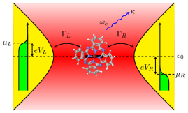
Model. Figure 1 shows a schematic of the system at hand. The Hamiltonian is written $H=H_{\rm S}+H_{\rm I}+H_{\rm B}$, where

$$H_{\rm S}=\tilde{\varepsilon}_{0}d^{\dagger}d^{\phantom{{\dagger}}}+\omega_{c}a^{\dagger}a+\Lambda_{\mathrm{m}}d^{\dagger}d(a+a^{\dagger}),$$ (1)

with $d^{\dagger}$ the creation operator for the electron on the dot single level of energy $\tilde{\varepsilon}_{0}$, $a^{\dagger}$ the creation operator for the photon field, and $\Lambda_{\mathrm{m}}=\lambda\omega_{c}$ the coupling constant. We follow Ref.Cottet et al. (2015) for the derivation of the interaction term sup . We neglect direct coupling of the cavity field to the electrons in the leads, since this effect is analogous to the coupling of the cavity field to the photon bath. We treat the electrons in the leads and the propagating electromagnetic modes as a bath: $H_{\rm B}=\sum_{\alpha k}\varepsilon_{\alpha k}c^{\dagger}_{\alpha k}c^{\phantom{{\dagger}}}_{\alpha k}+\sum_{q}\omega_{q}b^{\dagger}_{q}b^{\phantom{{\dagger}}}_{q}$, where $c^{\dagger}_{\alpha k}$ and $b^{\dagger}_{q}$ are the creation operators for the electrons on the leads $\alpha=L,R$ with energy $\varepsilon_{\alpha k}$ and for the propagating photons of energy $\omega_{q}$, respectively. The (linear) coupling to the bath is given by $H_{\rm I}=\sum_{\alpha k}\big{[}t_{\alpha k}c^{\dagger}_{\alpha k}d+t^{*}_{\alpha k}d^{\dagger}c^{\phantom{{\dagger}}}_{\alpha k}\big{]}+\sum_{q}\big{[}l_{q}a^{\dagger}b^{\phantom{{\dagger}}}_{q}+l^{*}_{q}b^{\dagger}_{q}a\big{]}$, with $t_{\alpha k}$ and $l_{q}$ the tunneling amplitudes. We first perform a standard Lang-Firsov unitary transformation on the Hamiltonian $\tilde{H}=UHU^{\dagger}$, with $U=e^{\lambda d^{\dagger}d(a-a^{\dagger})}$. This removes explicitly the electron-photon coupling term in $H_{\rm S}$, shifts the dot-level energy $\varepsilon_{0}=\tilde{\varepsilon}_{0}-\Lambda_{\mathrm{m}}^{2}/{\color[rgb]{0,0,0}\omega_{c}}$ and modifies the $d$ operator in $H_{\rm I}$ into $D=de^{\lambda(a-a^{\dagger})}$.

Figure 2: (a) Electronic current $I$ versus the voltage drops $V_{L}$ and $V_{R}$ for $\lambda=1.4$. (b) Current-voltage characteristics and (c) average photon occupation $\langle a^{\dagger}a\rangle$ in the cavity corresponding to the voltage profiles indicated in panel a (dashed and full lines) for different electron-photon coupling strengths $\lambda=0.1$ (blue), $\lambda=0.6$ (green) and $\lambda=1.4$ (magenta). The model parameters are $\kappa=10k_{B}T=0.1\omega_{c}$ and $\Gamma_{L}=\Gamma_{R}=\Gamma/2=10^{-3}\omega_{c}$.

Figure 3: Degree of coherence $g^{(2)}(0)$ for different electron-photon coupling strengths (a) $\lambda=0.1$, (b) $\lambda=0.6$, and (c) $\lambda=1.4$, respectively. The black dashed lines mark the contour $g^{(2)}(0)=1$ delimiting the regions of anti-bunching (blue areas). The model parameters are $\kappa=k_{B}T=0.1\omega_{c}$ and $\Gamma_{L}=\Gamma_{R}=10^{-3}\omega_{c}$.

Master-equation. Let us define the reduced density matrix $\rho(t)$ for the $d$ and $a$ degrees of freedom after tracing out the bath. We assume that the molecule is sufficiently isolated from the substrate, as is reasonable for STM experiments performed on thin insulating films Qiu et al. (2003); Zhang et al. (2016, 2017); Imada et al. (2017); Doppagne et al. (2018). We consider then the relevant regime $\Gamma\ll k_{B}T\ll\omega_{c}$ where the dynamics of $\rho(t)$ can be described by the Born-Markov master equation:

$$\dot{\rho}(t)=\mathcal{L}\rho(t)=-i[\tilde{H}_{\rm S},\rho(t)]+\left(\mathcal{L}_{\mathrm{c}}+\mathcal{L}_{e}\right)\rho(t).$$ (2)

The first term contributing to the Liouvilian operator $\mathcal{L}$ gives the coherent evolution of $\rho(t)$. The second one describes the damping of the cavity mode Louisell (1973); Gardiner and Collett (1985): $\mathcal{L}_{\mathrm{c}}\rho(t)=\kappa\left(2a\rho(t)a^{\dagger}-a^{\dagger}a\rho(t)-\rho(t)a^{\dagger}a\right)/2-\kappa n_{B}\left[a^{\dagger},\left[a,\rho(t)\right]\right]$, with $n_{B}(\omega_{c})=\left\{e^{\omega_{c}/k_{B}T}-1\right\}^{-1}$ the Bose distribution of photons in the bath at the cavity frequency. The last term describes incoherent electron tunneling $\mathcal{L}_{e}\rho(t)=\left[\mathcal{D}_{-}\rho(t)-\rho(t)\mathcal{D}_{+},D^{\dagger}\right]+\mbox{h.c.}$ Avriller et al. (2018), where $\mathcal{D}_{\pm}=\int_{-\infty}^{\infty}d\omega\int_{0}^{\infty}dt\Gamma_{\alpha}(\omega)f_{\alpha}^{\pm}(\omega)e^{i\omega t}D_{\rm{I}}(-t),$ and $\Gamma_{\alpha}=2\pi\sum_{k}|t_{\alpha k}|^{2}\delta(\omega-\varepsilon_{\alpha k})$ is the tunneling rate from the lead $\alpha$, that in the usual wide-band approximation becomes $\omega$-independent. Finally, $D_{\rm{I}}(-t)$ is the $D$ operator in the interaction representation with respect to $\tilde{H}_{\mathrm{S}}$. We introduced the short-hand notation $f^{+}_{\alpha}\left(\omega\right)=1-f^{-}_{\alpha}\left(\omega\right)=n_{F}(\omega-\mu_{\alpha})$, with $\mu_{\alpha}$ the chemical potential of lead $\alpha$ and $n_{F}(\omega)=\left\{e^{\omega/k_{B}T}+1\right\}^{-1}$ the Fermi distribution. The average or the correlation function of any observable $A$, $B$, can then be calculated in the stationary regime by $\left\langle A\right\rangle=\mathrm{Tr}[A\rho^{\mathrm{st}}]$ and $S_{AB}(t)=\left\langle A(t)B(0)\right\rangle=\mathrm{Tr}[Ae^{\mathcal{L}t}B\rho^{\mathrm{st}}]$ Cohen-Tannoudji et al. (1998); Kirton et al. (2012), with $\rho^{\mathrm{st}}$ the stationary solution of Eq. (2).

Electronic current. Using the previous results, we derive the expression for the average electronic dc-current evaluated at lead $\alpha$

$$I_{\alpha}=\frac{e\Gamma_{\alpha}}{\pi}\,\mathrm{Re}\!\!\int_{-\infty}^{\infty}\!\!d\omega\left\{f^{+}_{\alpha}(\omega)S_{DD^{\dagger}}(\omega)\!+\!f^{-}_{\alpha}(\omega)S_{D^{{\dagger}}D}(\omega)\right\}$$ (3)

where we introduced the Fourier transform of $f^{\pm}_{\alpha}$, $S_{DD^{\dagger}}$ and $S_{D^{\dagger}D}$. Equation (3) enables to calculate the current in presence of strong damping rates $\kappa$, that for plasmonic cavities reaches low quality factors $\omega_{c}/\kappa\approx 10$ Chikkaraddy et al. (2016). It allows to include the damping of the electromagnetic field during the tunneling process. This expression and $\rho^{\rm st}$ can be evaluated numerically by projecting on the charge and harmonic oscillator basis.

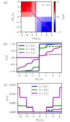
Figure 2(a) reports the electronic current $I$ for strong coupling, $\lambda=1.4$, as a function of the relative voltage drops $eV_{\alpha}=\mu_{\alpha}-\varepsilon_{0}$ between the chemical potential of lead $\alpha$ and the dot energy level cur . Specific current-voltage characteristics, corresponding to symmetric ($V_{L}=-V_{R}$) and asymmetric ($eV_{R}=-0.2\omega_{c}$) voltage drops, are shown respectively as full and dashed lines in Fig. 2(b), for weak ($\lambda=0.1$), moderate ($\lambda=0.6$), and strong ($\lambda=1.4$) coupling strengths. These exhibit similar features of the Franck–Condon blockade regime Koch and von Oppen (2005); Koch et al. (2006); Braig and Flensberg (2003), with inelastic steps observed each time the voltage drop $eV_{L}=n\omega_{c}$ matches a multiple of the cavity-photon frequency. This is the threshold for one-electron tunneling while emitting $n$ photons in the cavity. The step heights are given by the Poisson distribution $\mathcal{P}_{n}(\lambda)=e^{-\lambda^{2}}\lambda^{2n}/n!$ and the width of the inelastic steps by the cavity-losses $\kappa$, which exceed the temperature broadening. This is analogous to the broadening of phonon sidebands by frictional damping Braig and Flensberg (2003), but our treatment is not bound to thermal equilibrium.

Emitted light. We consider now the emitted light power $\sim\kappa\omega_{c}\langle a^{\dagger}a\rangle$, by plotting the average population of the cavity mode in Fig. 2(c) as a function of $V_{L}$. We find that the photon population also increases with bias voltage in a step-like manner bro , correlated to the evolution of the electronic current Avriller et al. (2018), thus confirming that single-electron tunneling is at the origin of light-emission inside the cavity. From Eq. (2), performing a secular approximation, we derive a rate equation for the photon population $P_{n}(t)$ sup . A relevant experimental regime in plasmonic cavities is $\kappa\gg\Gamma$ and $\omega_{c}\gg k_{B}T$. Since the time between two tunneling events is much longer than the damping time of the cavity, typically the circulating photon leaks out before a new photon is emitted in the cavity. In this limit $P_{0}\approx 1$, and we find for the other populations $P_{n}=\Gamma_{0n}/n\kappa\ll 1$, with $\Gamma_{0n}=\sum_{\alpha}\Gamma_{\alpha}\mathcal{P}_{n}(\lambda)\,n_{F}(n\omega_{c}-\mu_{\alpha})$ the cavity 0 to $n$-photons transition rate induced by a single tunneling event. The expression for $\langle a^{\dagger}a\rangle=\sum_{n}\Gamma_{0n}/\kappa$ describes then accurately the emitted power.

Figure 4: (a), (b) Role of temperature $T$ on the degree of coherence $g^{(2)}(0)$ for $V_{L}=-V_{R}$ with (a) $\lambda=0.1$ and (b) $\lambda=1.4$. Blue and magenta thick lines are slices from Fig. 3(a,c), while the orange ones are computed from rate equations sup . Dashed (dotted) horizontal line indicates $g^{(2)}(0)=2$ $(1)$ for thermal (uncorrelated) photon emission. (c) Minimum value of $g^{(2)}(0)$ (thick blue line) on the plane $(V_{L},V_{R})$, for fixed $\lambda$ and $k_{B}T=0.1\omega_{c}$. Dashed magenta line shows that minimum constrained to $V_{L}=-V_{R}$. Dashed black line gives the $T=0$ analytical prediction $(\lambda^{2}-2)^{2}/2$. Other parameters are those of Fig. 3.

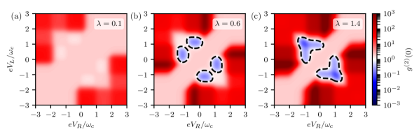
Correlation function $g^{(2)}$. In order to characterize the statistics of the emitted light, we compute the second-order correlation function $g^{(2)}(t)=\langle a^{\dagger}a^{\dagger}(t)a(t)a\rangle/\langle a^{\dagger}a\rangle^{2}$ Walls and Milburn (2008); Louisell (1973); Rice and Carmichael (1988); Glauber (1963). Let us begin with the $t=0$ case, $g^{(2)}(0)=(\sum_{n}n(n-1)P_{n})/(\sum_{n}nP_{n})^{2}$. One can readily verify that in thermal equilibrium $g^{(2)}(0)=2$. On Fig. 3 we show $g^{(2)}(0)$ as a function of $V_{R}$ and $V_{L}$, for three different values of $\lambda$. As expected, for $e|V_{L}-V_{R}|\ll k_{B}T$, one always finds the value of 2, corresponding to thermal equilibrium (pink regions on the diagonal $V_{L}=V_{R}$). Out of equilibrium we find either bunching $g^{(2)}(0)>1$ or anti-bunching $g^{(2)}(0)<1$. The anti-bunching appears for sufficiently strong coupling and is indicated by the blue regions with dashed border (where $g^{(2)}(0)=1$). Treating both the electron tunneling and the thermal excitations as weak perturbation to the distribution $P_{n}=\delta_{n,0}$ we obtain an analytical expression for $g^{(2)}(0)$ (see sup ) for voltages $eV_{L}=-eV_{R}\leq 2\omega_{c}$.

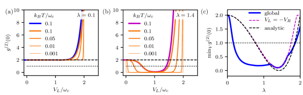
The prediction of this expression agrees very well with the numerical calculations for $k_{B}T\geq 0.1\omega_{c}$, (cf. thick lines in Fig. 4(a) and (b)). At lower temperature we thus show only the result obtained with the analytical expression, that does not suffer from numerical instability. In the strong coupling regime, we predict a smooth crossover from the equilibrium value $g^{(2)}(0)=2$ at low voltage, to an anti-bunching $g^{(2)}(0)<1$ regime that appears close to the first inelastic threshold ($|eV_{L}|\approx\omega_{c}$ or $|eV_{R}|\approx\omega_{c}$) sup ; Zou and Mandel (1990). As temperature decreases the region of anti-bunching expands, eventually including almost the full bias range $\left[0,2\omega_{c}\right]$, cf. Fig. 4(b).

Figure 4(c) shows the minimum value taken by $g^{(2)}(0)$ when minimized on the plane $(V_{L},V_{R})$ for a given value of the coupling $\lambda$. One finds that anti-bunching can be observed for $\lambda>0.17$ for an asymmetric bias configuration, thus being at reach of present experiments. The case of symmetric bias is also shown, with anti-bunching beginning at $\lambda>0.76$. Let us discuss now the anti-bunching mechanism for symmetric bias. When $P_{n+1}\ll P_{n}$, at lowest order $g^{(2)}(0)=2P_{2}/P_{1}^{2}$. This expression gives $2$ for thermal distribution $P_{n}\sim e^{-n\omega_{c}/k_{B}T}$. Anti-bunching is thus achieved for $2P_{2}\ll P_{1}^{2}$. At very low temperature the only way to populate the state $2$ is either a 2-photons transition (for $eV_{L}>2\omega_{c}$), or an electron-tunneling assisted transition from the state 1 to the state 2, controlled by $\Gamma_{12}=e^{-\lambda^{2}}\lambda^{2}\left(2-\lambda^{2}\right)^{2}\sum_{\alpha}\Gamma_{\alpha}n_{F}(\omega_{c}-\mu_{\alpha})/2$ (for $eV_{L}>\omega_{c}$). As a confirmation one finds that $P_{1}\approx P_{0}\Gamma_{01}/\kappa$ and $P_{2}\approx P_{1}\Gamma_{12}/2\kappa$, testifying that the result is just due to a balance between the light leaked out of the cavity and the photons emitted in the cavity by the tunneling electrons. From the explicit expression of $\Gamma_{12}$ at low temperature ($k_{B}T\ll\omega_{c}$) one then finds that the minimum value of $g^{(2)}(0)$ is approximated by $\left(\lambda^{2}-2\right)^{2}/2$ [dashed black line in Fig. 4(c)], tracing the $\lambda$-dependence of $\Gamma_{12}$. Its vanishing for $\lambda=\sqrt{2}$ is thus at the origin of the anti-bunching. A similar effect has also been recently reported in dc-biased Josephson junction coupled to microwave resonators Rolland et al. (2019); Grimm et al. (2019).

For larger voltages $eV_{L}\geq 2\omega_{c}$, we obtain analytically sup $g^{(2)}(0)\approx\kappa/2\Gamma$, as predicted by the numerical simulations giving a smooth evolution to strong bunching. This result agrees with the infinite bias voltage limit result recently reported in Ref. van den Berg and Samuelsson (2019). Finally the time dependence of $g^{(2)}(t)$ as obtained by the numerical calculations shows a smooth crossover on a time scale $1/\kappa$ from $g^{(2)}(0)=2$ to $g^{(2)}(\infty)=1$ (uncorrelated photons) Rice and Carmichael (1988). Only for $\lambda\approx 1$ we observe weak oscillations sup .

Conclusions. Charge fluctuations induced by electronic transport in a molecular single-electronic level are expected to couple strongly to the plasmonic mode formed by an STM tip and the substrate. We derived an expression for the current taking into account the strong damping of these cavities and obtained the current, emitted light intensity, and the correlation function $g^{(2)}(t)$. We showed that when the coupling strength is of the order $\lambda\sim 1$, Franck–Condon steps appear in both the current and the light intensity. Non-classical light can be emitted for a coupling strength in the range $0.17<\lambda<1.8$ for bias voltage near the one photon emission threshold. This prediction can be relevant for a series of experiments on STM cavities Reecht et al. (2014); Zhang et al. (2013); Merino et al. (2015); Zhang et al. (2016); Doppagne et al. (2018); Chong et al. (2018); Zhang et al. (2017); Imada et al. (2017); Neuman et al. (2018). The importance of single-level descriptions has further been reinforced experimentally after our initial submission Leon et al. (2019). The fast evolution of the cavity ($\kappa>k_{B}T$) might question the validity of the Markov approximation. We estimate that the non-Markovian contributions are negligible as far as $k_{B}T\ll\omega_{c}$, but investigating low-frequency response of plasmonic cavities could unravel such effects. Another interesting direction is the study of current response in presence of light irradiation of the plasmonic junction. Finally, we note that a local quantum emitter can be used to sense the environment of the molecule with the minimal quantum of energy.

Zou and Mandel (1990)

References

- Delbecq et al. (2011) M. R. Delbecq, V. Schmitt, F. D. Parmentier, N. Roch, J. J. Viennot, G. Fève, B. Huard, C. Mora, A. Cottet, and T. Kontos, Phys. Rev. Lett. 107, 256804 (2011).
- Bruhat et al. (2016) L. E. Bruhat, J. J. Viennot, M. C. Dartiailh, M. M. Desjardins, T. Kontos, and A. Cottet, Phys. Rev. X 6, 021014 (2016).
- Cottet et al. (2017) A. Cottet, M. C. Dartiailh, M. M. Desjardins, T. Cubaynes, L. C. Contamin, M. Delbecq, J. J. Viennot, L. E. Bruhat, B. Douçot, and T. Kontos, J. Phys.: Condens. Matter 29, 433002 (2017).
- Bruhat et al. (2018) L. E. Bruhat, T. Cubaynes, J. J. Viennot, M. C. Dartiailh, M. M. Desjardins, A. Cottet, and T. Kontos, Phys. Rev. B 98, 155313 (2018).
- Cubaynes et al. (2019) T. Cubaynes, M. R. Delbecq, M. C. Dartiailh, R. Assouly, M. M. Desjardins, L. C. Contamin, L. E. Bruhat, Z. Leghtas, F. Mallet, A. Cottet, and T. Kontos, npj Quantum Information 5, 47 (2019).
- Mi et al. (2017a) X. Mi, J. V. Cady, D. M. Zajac, P. W. Deelman, and J. R. Petta, Science 355, 156 (2017a).
- Mi et al. (2017b) X. Mi, J. V. Cady, D. M. Zajac, J. Stehlik, L. F. Edge, and J. R. Petta, Appl. Phys. Lett. 110, 043502 (2017b).
- Stockklauser et al. (2017) A. Stockklauser, P. Scarlino, J. V. Koski, S. Gasparinetti, C. K. Andersen, C. Reichl, W. Wegscheider, T. Ihn, K. Ensslin, and A. Wallraff, Phys. Rev. X 7, 011030 (2017).
- Liu et al. (2014) Y.-Y. Liu, K. D. Petersson, J. Stehlik, J. M. Taylor, and J. R. Petta, Phys. Rev. Lett. 113, 036801 (2014).
- Wallraff et al. (2004) A. Wallraff, D. I. Schuster, A. Blais, L. Frunzio, R.-S. Huang, J. Majer, S. Kumar, S. M. Girvin, and R. J. Schoelkopf, Nature 431, 162 (2004).
- Rolland et al. (2019) C. Rolland, A. Peugeot, S. Dambach, M. Westig, B. Kubala, Y. Mukharsky, C. Altimiras, H. le Sueur, P. Joyez, D. Vion, P. Roche, D. Esteve, J. Ankerhold, and F. Portier, Phys. Rev. Lett. 122, 186804 (2019).
- Grimm et al. (2019) A. Grimm, F. Blanchet, R. Albert, J. Leppäkangas, S. Jebari, D. Hazra, F. Gustavo, J.-L. Thomassin, E. Dupont-Ferrier, F. Portier, and M. Hofheinz, Phys. Rev. X 9, 021016 (2019).
- Berndt et al. (1991) R. Berndt, J. K. Gimzewski, and P. Johansson, Phys. Rev. Lett. 67, 3796 (1991).
- Qiu et al. (2003) X. H. Qiu, G. V. Nazin, and W. Ho, Science 299, 542 (2003).
- Schneider and Berndt (2012) N. L. Schneider and R. Berndt, Phys. Rev. B 86, 035445 (2012).
- Zhang et al. (2013) R. Zhang, Y. Zhang, Z. C. Dong, S. Jiang, C. Zhang, L. G. Chen, L. Zhang, Y. Liao, J. Aizpurua, Y. Luo, J. L. Yang, and J. G. Hou, Nature 498, 82 (2013).
- Reecht et al. (2014) G. Reecht, F. Scheurer, V. Speisser, Y. J. Dappe, F. Mathevet, and G. Schull, Phys. Rev. Lett. 112, 047403 (2014).
- Merino et al. (2015) P. Merino, C. Große, A. Roslawska, K. Kuhnke, and K. Kern, Nat. Commun. 6, 8461 (2015).
- Zhang et al. (2016) Y. Zhang, Y. Luo, Y. Zhang, Y.-J. Yu, Y.-M. Kuang, L. Zhang, Q.-S. Meng, Y. Luo, J.-L. Yang, Z.-C. Dong, and J. G. Hou, Nature 531, 623 (2016).
- Zhang et al. (2017) L. Zhang, Y.-J. Yu, L.-G. Chen, Y. Luo, B. Yang, F.-F. Kong, G. Chen, Y. Zhang, Q. Zhang, Y. Luo, J.-L. Yang, Z.-C. Dong, and J. G. Hou, Nat. Commun. 8, 580 (2017).
- Imada et al. (2017) H. Imada, K. Miwa, M. Imai-Imada, S. Kawahara, K. Kimura, and Y. Kim, Phys. Rev. Lett. 119, 013901 (2017).
- Doppagne et al. (2018) B. Doppagne, M. C. Chong, H. Bulou, A. Boeglin, F. Scheurer, and G. Schull, Science 361, 251 (2018).
- Chong et al. (2018) M. C. Chong, N. Afshar-Imani, F. Scheurer, C. Cardoso, A. Ferretti, D. Prezzi, and G. Schull, Nano Lett. 18, 175 (2018).
- Neuman et al. (2018) T. Neuman, R. Esteban, D. Casanova, F. J. Garcia-Vidal, and J. Aizpurua, Nano Lett. 18, 2358 (2018).
- Orgiu et al. (2015) E. Orgiu, J. George, J. A. Hutchison, E. Devaux, J. F. Dayen, B. Doudin, F. Stellacci, C. Genet, J. Schachenmayer, C. Genes, G. Pupillo, P. Samorì, and T. W. Ebbesen, Nat. Mater. 14, 1123 (2015).
- Schwartz et al. (2011) T. Schwartz, J. A. Hutchison, C. Genet, and T. W. Ebbesen, Phys. Rev. Lett. 106, 196405 (2011).
- Hagenmüller et al. (2017) D. Hagenmüller, J. Schachenmayer, S. Schütz, C. Genes, and G. Pupillo, Phys. Rev. Lett. 119, 223601 (2017).
- Chen et al. (2016) Z. Chen, Y. Zhou, and J.-T. Shen, Opt. Lett. 41, 3313 (2016).
- Chen et al. (2017) Z. Chen, Y. Zhou, and J.-T. Shen, Phys. Rev. A 96, 053805 (2017).
- Zhou et al. (2019) Y. Zhou, Z. Chen, L. V. Wang, and J.-T. Shen, Opt. Lett. 44, 475 (2019).
- Chikkaraddy et al. (2016) R. Chikkaraddy, B. de Nijs, F. Benz, S. J. Barrow, O. A. Scherman, E. Rosta, A. Demetriadou, P. Fox, O. Hess, and J. J. Baumberg, Nature 535, 127 (2016).
- Cottet et al. (2015) A. Cottet, T. Kontos, and B. Douçot, Phys. Rev. B 91, 205417 (2015).
- (33) See Supplemental Material at […] for the detailed derivation of the microscopic Hamiltonian, analysis of the electronic current and derivation of analytical formulas for the second-order correlation function of the cavity plasmon field which includes Cottet et al. (2015); Koch and von Oppen (2005); Burzurí et al. (2014); Pistolesi and Labarthe (2007); Cohen-Tannoudji et al. (1998); Zou and Mandel (1990) .
- Altimiras et al. (2013) C. Altimiras, O. Parlavecchio, P. Joyez, D. Vion, P. Roche, D. Esteve, and F. Portier, Appl. Phys. Lett. 103, 212601 (2013).
- Cassidy et al. (2017) M. C. Cassidy, A. Bruno, S. Rubbert, M. Irfan, J. Kammhuber, R. N. Schouten, A. R. Akhmerov, and L. P. Kouwenhoven, Science 355, 939 (2017).
- Braig and Flensberg (2003) S. Braig and K. Flensberg, Phys. Rev. B 68, 205324 (2003).
- Koch and von Oppen (2005) J. Koch and F. von Oppen, Phys. Rev. Lett. 94, 206804 (2005).
- Koch et al. (2006) J. Koch, F. von Oppen, and A. V. Andreev, Phys. Rev. B 74, 205438 (2006).
- Leturcq et al. (2009) R. Leturcq, C. Stampfer, K. Inderbitzin, L. Durrer, C. Hierold, E. Mariani, M. G. Schultz, F. von Oppen, and K. Ensslin, Nat. Phys. 5, 327 (2009).
- Burzurí et al. (2014) E. Burzurí, Y. Yamamoto, M. Warnock, X. Zhong, K. Park, A. Cornia, and H. S. van der Zant, Nano Lett. 14, 3191 (2014).
- Galperin and Nitzan (2005) M. Galperin and A. Nitzan, Phys. Rev. Lett. 95, 206802 (2005).
- Kaasbjerg and Nitzan (2015) K. Kaasbjerg and A. Nitzan, Phys. Rev. Lett. 114, 126803 (2015).
- Xu et al. (2016) F. Xu, C. Holmqvist, G. Rastelli, and W. Belzig, Phys. Rev. B 94, 245111 (2016).
- Louisell (1973) W. H. Louisell, Quantum statistical properties of radiation (Wiley, 1973).
- Gardiner and Collett (1985) C. W. Gardiner and M. J. Collett, Phys. Rev. A 31, 3761 (1985).
- Avriller et al. (2018) R. Avriller, B. Murr, and F. Pistolesi, Phys. Rev. B 97, 155414 (2018).
- Cohen-Tannoudji et al. (1998) C. Cohen-Tannoudji, J. Dupont-Roc, and G. Grynberg, Atom-Photon Interactions: Basic Processes and Applications (Wiley, 1998).
- Kirton et al. (2012) P. G. Kirton, A. D. Armour, M. Houzet, and F. Pistolesi, Phys. Rev. B 86, 081305(R) (2012).
- (49) We plot the symmetrized current , since for asymmetric bias voltages one observes in some cases weak non-conserving contributions.
- (50) At this level of approximation, the steps of the cavity-mode occupation appear to be broadened on the scale given by temperature instead of .
- Walls and Milburn (2008) D. F. Walls and G. J. Milburn, Quantum optics, 2nd ed. (Springer Berlin, 2008).
- Rice and Carmichael (1988) P. R. Rice and H. J. Carmichael, IEEE J. Quantum Electronics 24, 1351 (1988).
- Glauber (1963) R. J. Glauber, Phys. Rev. 131, 2766 (1963).
- Zou and Mandel (1990) X. T. Zou and L. Mandel, Phys. Rev. A 41, 475 (1990).
- van den Berg and Samuelsson (2019) T. L. van den Berg and P. Samuelsson, Phys. Rev. B 100, 035408 (2019).
- Leon et al. (2019) C. C. Leon, O. Gunnarsson, D. G. de Oteyza, A. Rosławska, P. Merino, A. Grewal, K. Kuhnke, and K. Kern, arXiv:1909.08117 (2019).
- Pistolesi and Labarthe (2007) F. Pistolesi and S. Labarthe, Phys. Rev. B 76, 165317 (2007).