Anisotropic magnetotransport in Dirac-Weyl magnetic junctions

Abstract

We theoretically study the anisotropic magnetotransport in Dirac-Weyl magnetic junctions where a doped ferromagnetic Weyl semimetal is sandwiched between doped Dirac semimetals. We calculate the conductance using the Landauer formula and find that the system exhibits extraordinarily large anisotropic magnetoresistance (AMR). The AMR depends on the ratio of the Fermi energy and the strength of the exchange interaction. The origin of the AMR is the shift of the Fermi surface in the Weyl semimetal and the mechanism is completely different from the conventional AMR originating from the spin dependent scattering and the spin-orbit interaction.

I Introduction

Magnetoresistance effects in ferromagnetic materials have been investigated during the past decades for applications to spintronics devices. Several kinds of magnetoresistance effects have been found. Anisotropic magnetoresistance (AMR) is a phenomenon where the resistance depends on the relative angle between the magnetization and the electric current McGuire and Potter (1975). Typically the angle dependent resistivity/conductivity is of the order of a few percent. Giant magnetoresistance (GMR) is another phenomenon observed in thin-film structures composed of alternating ferromagnetic and non-magnetic conductive layers Baibich et al. (1988); Binasch et al. (1989). In the GMR, the magnetoresistance exhibits several dozen percent, which significantly exceeds the AMR. Searching for stronger magnetoresistance effects such as the tunneling magnetoresistance Žutić et al. (2004) is a central issue in the field of spintronics.

Recently, magnetotransport in topological materials, such as topological insulators Hasan and Kane (2010); Qi and Zhang (2011) and Dirac/Weyl semimetals Young et al. (2012); Wang et al. (2012); Murakami (2007); Wan et al. (2011); Burkov and Balents (2011), have drawn much interest for achieving novel electromagnetic coupling via the strong spin-orbit interaction Yokoyama et al. (2010); Matsuzaki and Nomura (2015); Scharf et al. (2016). A Dirac semimetal manifests the pseudo-relativistic linear dispersions doubly degenerate with time-reversal and spatial-inversion symmetries, and it is non-magnetic Liu et al. (2014); Neupane et al. (2014); Borisenko et al. (2014). A Weyl semimetal possesses the gapless linear dispersions with broken time-reversal Liu et al. (2015); Wang et al. (2016); Borisenko (2016) or spatial-inversion symmetries Xu et al. (2015a); Lv et al. (2015); Xu et al. (2015b); Belopolski et al. (2015); Yang et al. (2015a); Xu et al. (2015c, 2016). In a magnetic Weyl semimetal, time reversal symmetry is broken because of a magnetic ordering. One of the signatures of Dirac/Weyl semimetals is the longitudinal negative magnetoresistance Nielsen and Ninomiya (1983); Aji (2012); Son and Spivak (2013); Burkov (2014); Gorbar et al. (2014); Lu et al. (2015); Burkov (2015) that has been observed experimentally in non-magnetic systems Xiong et al. (2015); Li et al. (2015); Zhang et al. (2015a); Huang et al. (2015); Zhang et al. (2015b); Yang et al. (2015b); Li et al. (2016); Arnold et al. (2016); Zhang et al. (2016); dos Reis et al. (2016). The negative magnetoresistance can be observed in both time-reversal and spatial-inversion symmetry broken Weyl semimetals. Here, we study magnetoresistance effects that is peculiar to the time-reversal symmetry broken Weyl semimetals, i.e., magnetic Weyl semimetals.

In this paper, we study the anisotropic magnetotransport in Dirac-Weyl magnetic junctions. We consider a system that consists of a doped ferromagnetic Weyl semimetal sandwiched by doped Dirac semimetals, and calculate the transmission probability through the Dirac-Weyl magnetic junctions. In our system, the Dirac/Weyl semimetals are characterized by the absence/presence of the spontaneous magnetization, which splits the band touching points in momentum space. Using the Landauer formula, we compute the conductance as a function of the relative angle between the magnetization and the electric current. We find that the AMR can be extraordinarily large compared with that of conventional ferromagnetic metals and the AMR has the same periodicity of the conventional AMR as a function of the relative angle. In the Dirac-Weyl magnetic junctions, the mechanism of the AMR is entirely different from the conventional one, which is generally considered to arise from spin dependent scattering and spin-orbit coupling. The shift of the Fermi surface caused by the magnetization in the Weyl semimetal is the origin of the AMR.

The paper is organized as follows. In Sec. II, we introduce a continuous model which describes a Dirac semimetal and a ferromagnetic Weyl semimetal with a pair of Weyl nodes. In Sec. III, we calculate the transmission probability of the Dirac-Weyl magnetic junctions. In Sec. IV, we compute the conductance using the Landauer formula. The conclusion and discussion are given in Sec. V.

II Model Hamiltonian

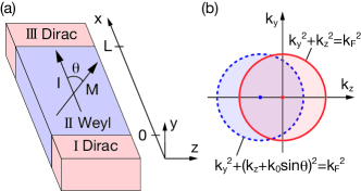
We consider magnetic junctions composed of Dirac and ferromagnetic Weyl semimetals as illustrated in Fig. 1(a), where the doped magnetic Weyl semimetal in region II $(0\leq x\leq L)$ is sandwiched between the doped Dirac semimetals in region I and III $(x<0,L<x)$. We assume that the Dirac semimetals are semi-infinite in $x$ direction and the system is periodic in $y$ and $z$ direction. The magnetic junction is implemented in the magnetization,

$$\bm{M}(x)=\begin{cases}\hskip 14.22636pt(0,0,0)\hskip 42.67912pt(x<0,L<x),\\ M_{0}(\cos\theta,0,\sin\theta)\hskip 14.22636pt(0\leq x\leq L),\end{cases}$$ (1)

as shown in Fig. 1(a).

Figure 1: (a) Dirac-Weyl magnetic junctions composed of Dirac and ferromagnetic Weyl semimetals. The magnetization vector is on the $x$-$z$ plane and the angle between the magnetization and the $x$ axis is $\theta$. (b) Fermi surfaces of Dirac and Weyl semimetals with positive chirality projected on $k_{y}$-$k_{z}$ plane. The area inside the red solid (blue dashed) circle represents the Fermi surface of the Dirac (Weyl) semimetal.

We start with a model Hamiltonian for electrons in Dirac/Weyl semimetals,

$$H_{0}=\hbar v\tau_{z}\bm{\sigma}\cdot(-i\bm{\nabla})+\tau_{0}J\bm{M}(x)\cdot\bm{\sigma},$$ (2)

where $v$ is the velocity, $\bm{\sigma}$ and $\bm{\tau}$ are the triplets of Pauli matrices acting on the real spin and the pseudospin (chirality) degrees of freedom, and $J$ is the exchange coupling constant. There are two nodes with positive and negative chirality characterizing the correlation between the spin and the momentum. In region I and III (doped Dirac semimetal), there is no magnetic moment, and the energy bands are doubly degenerate. In region II (doped Weyl semimetal), the exchange interaction splits the two-fold Fermi surfaces in the direction of the magnetization in momentum space. In the present work, we treat two Fermi surfaces with positive and negative chiralities independently, assuming the absence of inter-node scattering. Figure 1(b) shows the Fermi surfaces of the Dirac and Weyl semimetals with positive chirality, projected on $k_{y}$-$k_{z}$ plane. In the presence of the magnetization (in region II), the Fermi surface is shifted along the $k_{z}$ axis by $k_{0}\sin\theta$, where

$$k_{0}={JM_{0}\over\hbar v}.$$ (3)

When $k_{\rm F}>k_{0}\sin\theta$, where $k_{\rm F}$ is the Fermi wave number, the projected Fermi surfaces of the Dirac and Weyl semimetals are partially overlapped, while not when $k_{\rm F}<k_{0}\sin\theta$.

III Transmission probability

In this section, we calculate transmission probability along $x$ axis for eigenstates of the positive chirality. Due to the translational invariance along $y$ and $z$ axis, the wave numbers $k_{y}$ and $k_{z}$ are conserved and an eigenstate is labeled by the wave numbers $k_{y}$ and $k_{z}$ in the projected Fermi surface of the Dirac semimetals, $k_{y}^{2}+k_{z}^{2}<k_{\rm F}^{2}$. The common factor $e^{i(k_{y}y+k_{z}z)}$ is omitted in the following expressions.

The wave function can be written in terms of incident and reflected waves. In region I, the two-component wave function is written as

$$\psi_{\rm I}(x)= \begin{pmatrix}k_{x}-ik_{y}\\ k_{\rm F}-k_{z}\end{pmatrix}e^{ik_{x}x}$$

$$+r\begin{pmatrix}-k_{x}-ik_{y}\\ k_{\rm F}-k_{z}\end{pmatrix}e^{-ik_{x}x},$$ (4)

where

$$k_{x}=\sqrt{k_{\rm F}^{2}-k_{y}^{2}-k_{z}^{2}}\ .$$ (5)

In region II, we have

$$\psi_{\rm I\nobreak I}(x)= \hskip 11.38109pta\begin{pmatrix}k_{x}^{\prime}-ik_{y}\\ k_{\rm F}-(k_{z}+k_{0}\sin\theta)\end{pmatrix}e^{i(k_{x}^{\prime}-k_{0}\cos\theta)x}$$

$$+b\begin{pmatrix}-k_{x}^{\prime}-ik_{y}\\ k_{\rm F}-(k_{z}+k_{0}\sin\theta)\end{pmatrix}e^{i(-k_{x}^{\prime}-k_{0}\cos\theta)x},$$ (6)

where

$$k_{x}^{\prime}=\sqrt{k_{\rm F}^{2}-k_{y}^{2}-(k_{z}+k_{0}\sin\theta)^{2}}\ .$$ (7)

In the case of $k_{\rm F}^{2}-k_{y}^{2}-(k_{z}+k_{0}\sin\theta)^{2}<0$, $k_{x}^{\prime}$ becomes pure imaginary number, and the wave function describes an evanescent mode decaying exponentially. In region III, we have

$$\psi_{\rm I\nobreak I\nobreak I}(x)=t\begin{pmatrix}k_{x}-ik_{y}\\ k_{\rm F}-k_{z}\end{pmatrix}e^{ik_{x}x}.$$ (8)

The continuity of the wave functions at the junctions gives boundary conditions, $\psi_{\rm I}(0)=\psi_{\rm I\nobreak I}(0)$ and $\psi_{\rm I\nobreak I}(L)=\psi_{\rm I\nobreak I\nobreak I}(L)$, and determines the coefficients $r$, $a$, $b$, and $t$. The transmission probability along $x$ axis is obtained from $T(k_{y},k_{z},\theta)=|t|^{2}$ and has the form

$$T(k_{y},k_{z},\theta)=$$

$$\frac{4k_{x}^{2}k_{x}^{\prime\,2}}{4k_{x}^{2}k_{x}^{\prime\,2}\cos^{2}(k_{x}^{\prime}L)+\left(k_{x}^{2}\!+\!k_{x}^{\prime\,2}\!+\!k_{0}^{2}\sin^{2}\!\theta\right)^{\!2}\!\sin^{2}(k_{x}^{\prime}L)}.$$ (9)

Note that $k_{x}$ and $k_{x}^{\prime}$ are functions of $k_{y}$ and $k_{z}$ as given in Eqs. (5) and (7). From the above expression, we see that the transmission probability depends on the $z$ component of the magnetization, giving the shift of the projected Fermi surface, while the $x$ component does not contribute. Therefore, the transmission probability is unity at $\theta=m\pi$ with an integer $m$.

As shown in Fig. 1(b), the projected Fermi surface of the Dirac semimetals ($k_{y}^{2}+k_{z}^{2}<k_{\rm F}^{2}$) can be divided into two regions: overlapping region [$k_{y}^{2}\!+\!(k_{z}\!+\!k_{0}\sin\!\theta)^{2}\!<\!k_{\rm F}^{2}$], where that of the Weyl semimetal is overlapping, and non-overlapping region [$k_{y}^{2}+(k_{z}+k_{0}\sin\theta)^{2}\!>\!k_{\rm F}^{2}$], where the traveling mode corresponding to the incident wave is absent in the Weyl semimetal. The expression Eq. (9) is applicable also to a pure imaginary $k_{x}^{\prime}$, i.e., the wave function in region II is an evanescent mode. The transmission probability behaves in a significantly different manner in the overlapping (with real $k_{x}^{\prime}$) and non-overlapping (with pure imaginary $k_{x}^{\prime}$) regions.

In the overlapping region, the incident wave is transmitted via the traveling mode in region II. From Eq. (9), we can show that the incident wave is transmitted with the transmission probability $T(k_{y},k_{z},\theta)=1$ for values of $k_{x}^{\prime}L$ satisfying the relation $k_{x}^{\prime}L=n\pi$ Bai et al. (2016a, b); You et al. (2016); Yesilyurt et al. (2016); Siu et al. (2016), with $n$ a positive integer, corresponding to a condition that a standing wave can exist in the region II. The relation is written as

$$k_{y}^{2}+(k_{z}+k_{0}\sin\theta)^{2}=k_{\rm F}^{2}\left[1-\left(\frac{n\pi}{k_{\rm F}L}\right)^{2}\right].$$ (10)

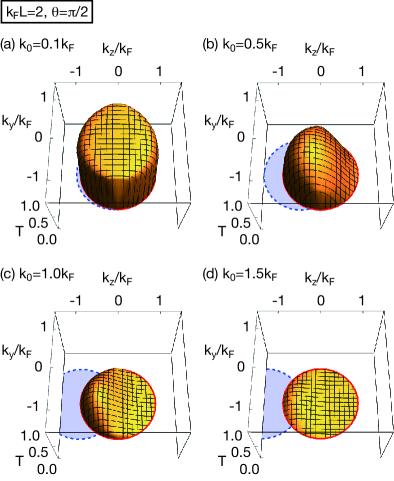
Figure 2 shows the transmission probability as a function of $k_{y}$ and $k_{z}$ at several $L$’s. We set $k_{0}=0.5k_{\rm F}$ and $\theta=\pi/2$ as a typical example. For $k_{\rm F}L<\pi$, there is no solution of Eq. (10), so that there is no peak structure in Fig. 2(a) and the transmission probability satisfies $T(k_{y},k_{z},\theta)<1$. In Figs. 2(b), (c), and (d), there are peak structures where the transmission probability is unity on the circles represented by Eq. (10). The number of peaks increases with the increase of $k_{\rm F}L$.

In the non-overlapping region, an evanescent mode in region II, $k_{x}^{\prime}=i\kappa$ with $\kappa=\sqrt{-k_{\rm F}^{2}+k_{y}^{2}+(k_{z}+k_{0}\sin\theta)^{2}}$, transmits an incident wave and the transmission probability is written as

$$T(k_{y},k_{z},\theta)=$$

$$\frac{4k_{x}^{2}{\kappa}^{2}}{4k_{x}^{2}{\kappa}^{2}\cosh^{2}(\kappa L)+\left(k_{x}^{2}\!-\!\kappa^{2}\!+\!k_{0}^{2}\sin^{2}\!\theta\right)^{2}\!\sinh^{2}(\kappa L)}.$$ (11)

From the above expression, we immediately see that the transmission probability monotonically decreases with the increase of $L$ in an exponential manner. Figure 2 shows that the transmission probability becomes exponentially small.

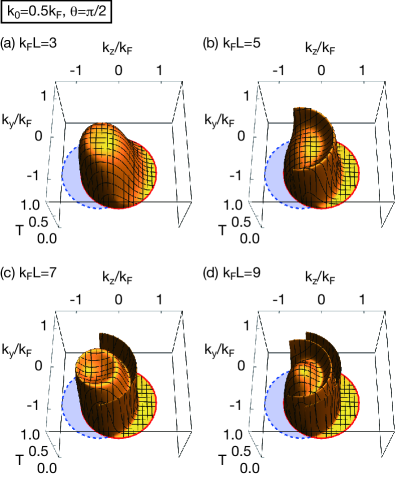
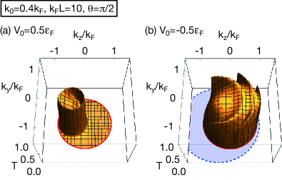
Figure 3 shows the transmission probability at several $k_{0}$’s, where we set $k_{\rm F}L=2$ and $\theta=\pi/2$. For a large $k_{0}$, the transmission probability is significantly suppressed even in the overlapping region; the spin-momentum locking causes the discrepancy of the spinors between the incident and traveling modes.

Figure 2: Transmission probability as a function of $k_{y}$ and $k_{z}$ in the Fermi surface of the Dirac semimetals projected on the $k_{y}$-$k_{z}$ plane. Transmission probability is plotted at (a) $k_{\rm F}L=3$, (b) $k_{\rm F}L=5$, (c) $k_{\rm F}L=7$, (d) $k_{\rm F}L=9$. We set $k_{0}=0.5k_{\rm F}$ and $\theta=\pi/2$.

Figure 3: Transmission probability as a function of $k_{y}$ and $k_{z}$ in the Fermi surface of the Dirac semimetals projected on the $k_{y}$-$k_{z}$ plane. Transmission probability is plotted at (a) $k_{0}=0.1k_{\rm F}$, (b) $k_{0}=0.5k_{\rm F}$, (c) $k_{0}=1.0k_{\rm F}$, (d) $k_{0}=1.5k_{\rm F}$. We set $k_{\rm F}L=2$ and $\theta=\pi/2$.

IV Conductance

To characterize the total transmission for the given magnetization direction and magnitude, we calculate the Landauer conductance

$$G(\theta)= 2\frac{e^{2}}{h}\sum_{k_{y}k_{z}}T(k_{y},k_{z},\theta)$$

$$= 2\frac{e^{2}}{h}\frac{S}{(2\pi)^{2}}\int_{D}T(k_{y},k_{z},\theta)dk_{y}dk_{z},$$ (12)

where $S$ is the area of the junctions, and the region $D$ is the projected Fermi surface of the Dirac semimetals, $k_{y}^{2}+k_{z}^{2}<k_{\rm F}^{2}$. The factor two comes from the two nodes with positive and negative chiralities giving the same contribution. The conductance $G(\theta)$ is naturally proportional to $S$, and the conductance per unit area, $G(\theta)/S$, can be used as a quantity that measures the transparency of the magnetic junctions for the electronic transport.

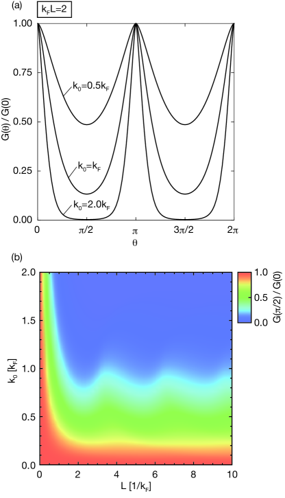
In Fig. 4(a), we plot the conductance, Eq. (12), as a function of $\theta$. Here, we set $k_{\rm F}L=2$ and $k_{0}=0.5k_{\rm F}$, $k_{\rm F}$, $2k_{\rm F}$. The conductance has a property, $G(\theta+\pi)=G(\theta)$, i.e., $G(\theta)$ has a periodicity of $\pi$, which can be derived from Eq. (9), the expression for $T(k_{y},k_{z},\theta)$, and appropriately changing the integral variable in Eq. (12). At the angles $\theta=m\pi$ with an integer $m$, the conductance is independent of $k_{0}$ and $\theta$, because the transmission probability is unity for the arbitrary incident wave as we mentioned in the previous section. The conductance decreases when the angle $\theta$ deviates from $\theta=m\pi$ and reaches a minimum value at $\theta=(m+1/2)\pi$. This is because the conductance is governed by the area of the overlapping region, and the overlapping area depends only on the shift of the projected Fermi surface $|k_{0}\sin\theta|$. Therefore, the conductance decreases with the increase of $k_{0}$, as we can see it in Fig. 4(a). At $k_{0}=2k_{\rm F}$, there is no overlapping region at $\theta=(m+1/2)\pi$, so that the conductance becomes exponentially small.

In Fig. 4(b), the conductance $G(\pi/2)$, which is the minimum value of $G(\theta)$, is plotted as a function of $L$ and $k_{0}$. When $k_{0}$ is fixed, the conductance decreases with the increase of $L$ because the transmission probability in the non-overlapping region decreases exponentially, and approaches to a minimum value, which is approximately proportional to the area of the overlapping region. Around $k_{0}\approx 0.7k_{\rm F}$, we see oscillatory behavior coming from the peak structures of the transmission probability. The conductance at fixed $L$ decreases with the increase of $k_{0}$ because of the decrease of the overlapping area.

Figure 4: (a) The conductance $G(\theta)$ as a function of $\theta$. We set $k_{\rm F}L=2$ and plot the conductance for $k_{0}=0.5k_{\rm F},k_{\rm F},2.0k_{\rm F}$. (b) The color plot of the ratio of the conductance $G(\pi/2)/G(0)$ as a function of $L$ and $k_{0}$.

V Conclusion and Discussion

We studied the anisotropic magnetotransport in the Dirac-Weyl magnetic junctions and found that the present system exhibits the extraordinarily large AMR. For the magnetization parallel to the electric current ($\theta=0$), the conductance is not influenced by the magnetization, while for the magnetization perpendicular to the electric current ($\theta=\pi/2$), the conductance becomes exponentially small for a sufficiently strong exchange interaction and magnetization, i.e., $k_{0}\gg k_{\rm F}$.

Here we discuss the case when the sizes of the Fermi surface in the Dirac and Weyl semimetals are different, and show that the difference does’t change the qualitative results. In this paper, we have assumed that the sizes of the Fermi surface are the same, although they can be different in general. In this case, the Hamiltonian is given as

$$H=H_{0}+V(x),$$ (13)

where $V(x)$ is a potential, shifting the Fermi energy of the Weyl semimetal,

$$V(x)=\begin{cases}0\hskip 13.65732pt(x<0,L<x),\\ V_{0}\hskip 8.53581pt(0\leq x\leq L).\end{cases}$$ (14)

In a similar manner to Eq. (9), we derive the transmission probability,

$$T(k_{y},k_{z},\theta)=$$

$$\frac{4k_{x}^{2}k_{x}^{\prime\,2}}{4k_{x}^{2}k_{x}^{\prime\,2}\cos^{2}(k_{x}^{\prime}L)+\left[k_{x}^{2}\!+\!k_{x}^{\prime\,2}\!+\!k_{0}^{2}\sin^{2}\!\theta-V_{0}^{2}/(\hbar v)^{2}\right]^{\!2}\!\sin^{2}(k_{x}^{\prime}L)},$$ (15)

where

$$k_{x}^{\prime} =\sqrt{\left[k_{\rm F}-V_{0}/(\hbar v)\right]^{2}-k_{y}^{2}-(k_{z}+k_{0}\sin\theta)^{2}}\ .$$ (16)

In Fig. 5, the transmission probability is plotted at (a) $V_{0}=0.5\varepsilon_{\rm F}$ and (b) $V_{0}=-0.5\varepsilon_{\rm F}$, where $\varepsilon_{\rm F}=\hbar vk_{\rm F}$. We again observe the peak structures on $k_{x}^{\prime}L=n\pi$ and the suppression of the transmission probability originating from the spin-momentum locking.

Figure 5: Transmission probability as a function of $k_{y}$ and $k_{z}$ in the Fermi surface of the Dirac semimetals projected on the $k_{y}$-$k_{z}$ plane. Transmission probability is plotted at (a) $V_{0}=0.5\varepsilon_{\rm F}$ and (b) $V_{0}=-0.5\varepsilon_{\rm F}$, where $\varepsilon_{\rm F}=\hbar vk_{\rm F}$. We set $k_{0}=0.4k_{\rm F}$, $k_{\rm F}L=10$, and $\theta=\pi/2$.

The origin of the AMR in the present system is the shift of the Fermi surface in the momentum space, which is completely different from that of the conventional AMR in ferromagnetic metal, but we can get an expression for the conductance that resembles the conventional AMR. On condition that $|k_{0}\sin\theta|$ is much smaller than the Fermi wave number $k_{\rm F}$, the transmission probability Eq. (9) is approximated by

$$T(k_{y},k_{z},\theta)\simeq 1-T_{1} (k_{y},k_{z})\left(\frac{k_{0}\sin\theta}{k_{\rm F}}\right)$$

$$-T_{2}(k_{y},k_{z})\left(\frac{k_{0}\sin\theta}{k_{\rm F}}\right)^{2},$$ (17)

where we neglect higher order terms than $(k_{0}\sin\theta/k_{\rm F})^{2}$. Substituting Eq. (17) for Eq. (12), we get an approximate expression. The conductance $G(\theta)$ is an even function of $\theta$, i.e., $G(\theta)=G(-\theta)$, because the system with the relative angle $-\theta$ can be transformed into the relative angle $\theta$ by rotating the system around $x$ axis. Therefore, the conductance is written as

$$G(\theta)\simeq G(0)-\Delta G\sin^{2}\theta,$$ (18)

where

$$G(0)=2\frac{e^{2}}{h}\frac{S}{(2\pi)^{2}}\pi k_{\rm F}^{2},$$

$$\Delta G=2\frac{e^{2}}{h}\frac{S}{(2\pi)^{2}}\int_{D}T_{2}(k_{y},k_{z})\left(\frac{k_{0}}{k_{\rm F}}\right)^{2}dk_{y}dk_{z}.$$ (19)

The above expression for $G(\theta)$ is similar to the AMR in the conventional ferromagnetic metals McGuire and Potter (1975).

Finally, we mention how to observe the extraordinarily large AMR experimentally. There is a great deal of theoretical and experimental work on searching for magnetic Weyl semimetals. One of the candidate materials is Cr-doped ${\rm Bi}_{2}({\rm Se}_{x}{\rm Te}_{1-x})_{3}$ Chen et al. (2010); Zhang et al. (2013); Kurebayashi and Nomura (2014). The bulk band gap of ${\rm Bi}_{2}{\rm Se}_{3}$ can be tuned by substituting tellurium for selenium, and the gap almost closes at the $\Gamma$ point with the selenium concentration $x\simeq 0.6$ Sato et al. (2011); Jin et al. (2011). In the presence of magnetic dopants Cr, we expect the ferromagnetic ordering below a critical temperature and emergence of the Weyl semimetal phase. Therefore, the AMR discussed in the present work can be observed in multilayer structure of non-magnetic and magnetic ${\rm Bi}_{2}({\rm Se}_{x}{\rm Te}_{1-x})_{3}$. The condition to observe the large AMR is written as $k_{\rm F}\ll k_{0}$ and $L\gg 1/k_{\rm F}$. Using the parameters for the above material ($JM_{0}=2.0x_{i}S[{\rm eV}],\hbar v=2.2[{\rm eV\AA}]$) Yu et al. (2010); Chen et al. (2010); Zhang et al. (2013, 2009); Liu et al. (2010), where $x_{i}$ is the ratio of the magnetic dopants and $S=3/2$, we can quantitatively estimate the shift of the Fermi surface $k_{0}$. At $x_{i}=0.1$, the condition is satisfied when $k_{\rm F}\ll 0.14[{\rm\AA}^{-1}](\varepsilon_{\rm F}\ll 0.31[{\rm eV}])$. In this situation, we can set $k_{\rm F}=0.01[{\rm\AA}^{-1}]$ as a typical value, so that the condition for the system size is written as $L\gg 100[{\rm\AA}]$.

References

- McGuire and Potter (1975) T. McGuire and R. Potter, IEEE Transactions on Magnetics 11, 1018 (1975).
- Baibich et al. (1988) M. N. Baibich, J. M. Broto, A. Fert, F. N. Van Dau, F. Petroff, P. Etienne, G. Creuzet, A. Friederich, and J. Chazelas, Physical review letters 61, 2472 (1988).
- Binasch et al. (1989) G. Binasch, P. Grünberg, F. Saurenbach, and W. Zinn, Physical review B 39, 4828 (1989).
- Žutić et al. (2004) I. Žutić, J. Fabian, and S. D. Sarma, Reviews of modern physics 76, 323 (2004).
- Hasan and Kane (2010) M. Z. Hasan and C. L. Kane, Reviews of Modern Physics 82, 3045 (2010).
- Qi and Zhang (2011) X.-L. Qi and S.-C. Zhang, Reviews of Modern Physics 83, 1057 (2011).
- Young et al. (2012) S. M. Young, S. Zaheer, J. C. Teo, C. L. Kane, E. J. Mele, and A. M. Rappe, Physical review letters 108, 140405 (2012).
- Wang et al. (2012) Z. Wang, Y. Sun, X.-Q. Chen, C. Franchini, G. Xu, H. Weng, X. Dai, and Z. Fang, Physical Review B 85, 195320 (2012).
- Murakami (2007) S. Murakami, New Journal of Physics 9, 356 (2007).
- Wan et al. (2011) X. Wan, A. M. Turner, A. Vishwanath, and S. Y. Savrasov, Physical Review B 83, 205101 (2011).
- Burkov and Balents (2011) A. Burkov and L. Balents, Physical review letters 107, 127205 (2011).
- Yokoyama et al. (2010) T. Yokoyama, Y. Tanaka, and N. Nagaosa, Physical Review B 81, 121401 (2010).
- Matsuzaki and Nomura (2015) I. Matsuzaki and K. Nomura, arXiv preprint arXiv:1503.04953 (2015).
- Scharf et al. (2016) B. Scharf, A. Matos-Abiague, J. E. Han, E. M. Hankiewicz, and I. Žutić, Phys. Rev. Lett. 117, 166806 (2016).
- Liu et al. (2014) Z. Liu, B. Zhou, Y. Zhang, Z. Wang, H. Weng, D. Prabhakaran, S.-K. Mo, Z. Shen, Z. Fang, X. Dai, et al., Science 343, 864 (2014).
- Neupane et al. (2014) M. Neupane, S.-Y. Xu, R. Sankar, N. Alidoust, G. Bian, C. Liu, I. Belopolski, T.-R. Chang, H.-T. Jeng, H. Lin, et al., Nature communications 5 (2014).
- Borisenko et al. (2014) S. Borisenko, Q. Gibson, D. Evtushinsky, V. Zabolotnyy, B. Büchner, and R. J. Cava, Physical review letters 113, 027603 (2014).
- Liu et al. (2015) J. Liu, J. Hu, D. Graf, S. Radmanesh, D. Adams, Y. Zhu, G. Chen, X. Liu, J. Wei, I. Chiorescu, et al., arXiv preprint arXiv:1507.07978 (2015).
- Wang et al. (2016) Y.-Y. Wang, Q.-H. Yu, and T.-L. Xia, arXiv preprint arXiv:1603.09117 (2016).
- Borisenko (2016) S. Borisenko, arXiv preprint arXiv:1507.04847 (2016).
- Xu et al. (2015a) S.-Y. Xu, I. Belopolski, N. Alidoust, M. Neupane, G. Bian, C. Zhang, R. Sankar, G. Chang, Z. Yuan, C.-C. Lee, et al., Science 349, 613 (2015a).
- Lv et al. (2015) B. Lv, H. Weng, B. Fu, X. Wang, H. Miao, J. Ma, P. Richard, X. Huang, L. Zhao, G. Chen, et al., Phys. Rev. X 5, 031013 (2015).
- Xu et al. (2015b) S.-Y. Xu, N. Alidoust, I. Belopolski, Z. Yuan, G. Bian, T.-R. Chang, H. Zheng, V. N. Strocov, D. S. Sanchez, G. Chang, et al., Nature Physics (2015b).
- Belopolski et al. (2015) I. Belopolski, S.-Y. Xu, D. Sanchez, G. Chang, C. Guo, M. Neupane, H. Zheng, C.-C. Lee, S.-M. Huang, G. Bian, et al., arXiv preprint arXiv:1509.07465 (2015).
- Yang et al. (2015a) L. Yang, Z. Liu, Y. Sun, H. Peng, H. Yang, T. Zhang, B. Zhou, Y. Zhang, Y. Guo, M. Rahn, et al., Nature physics 11, 728 (2015a).
- Xu et al. (2015c) S.-Y. Xu, I. Belopolski, D. S. Sanchez, C. Zhang, G. Chang, C. Guo, G. Bian, Z. Yuan, H. Lu, T.-R. Chang, et al., Science advances 1, e1501092 (2015c).
- Xu et al. (2016) N. Xu, H. Weng, B. Lv, C. Matt, J. Park, F. Bisti, V. Strocov, E. Pomjakushina, K. Conder, N. Plumb, et al., Nature communications 7, 11006 (2016).
- Nielsen and Ninomiya (1983) H. B. Nielsen and M. Ninomiya, Phys. Lett. B 130, 389 (1983).
- Aji (2012) V. Aji, Phys. Rev. B 85, 241101 (2012).
- Son and Spivak (2013) D. T. Son and B. Z. Spivak, Phys. Rev. B 88, 104412 (2013).
- Burkov (2014) A. Burkov, Phys. Rev. Lett. 113, 247203 (2014).
- Gorbar et al. (2014) E. Gorbar, V. Miransky, and I. Shovkovy, Phys. Rev. B 89, 085126 (2014).
- Lu et al. (2015) H.-Z. Lu, S.-B. Zhang, and S.-Q. Shen, Phys. Rev. B 92, 045203 (2015).
- Burkov (2015) A. Burkov, Phys. Rev. B 91, 245157 (2015).
- Xiong et al. (2015) J. Xiong, S. K. Kushwaha, T. Liang, J. W. Krizan, M. Hirschberger, W. Wang, R. Cava, and N. Ong, Science 350, 413 (2015).
- Li et al. (2015) C.-Z. Li, L.-X. Wang, H. Liu, J. Wang, Z.-M. Liao, and D.-P. Yu, Nature communications 6, 10137 (2015).
- Zhang et al. (2015a) C. Zhang, E. Zhang, Y. Liu, Z.-G. Chen, S. Liang, J. Cao, X. Yuan, L. Tang, Q. Li, T. Gu, et al., arXiv preprint arXiv:1504.07698 (2015a).
- Huang et al. (2015) X. Huang, L. Zhao, Y. Long, P. Wang, D. Chen, Z. Yang, H. Liang, M. Xue, H. Weng, Z. Fang, et al., Physical Review X 5, 031023 (2015).
- Zhang et al. (2015b) C. Zhang, S.-Y. Xu, I. Belopolski, Z. Yuan, Z. Lin, B. Tong, N. Alidoust, C.-C. Lee, S.-M. Huang, H. Lin, et al., Preprint at http://arxiv. org/abs/1503.02630 (2015b).
- Yang et al. (2015b) X. Yang, Y. Liu, Z. Wang, Y. Zheng, and Z.-a. Xu, arXiv preprint arXiv:1506.03190 (2015b).
- Li et al. (2016) H. Li, H. He, H.-Z. Lu, H. Zhang, H. Liu, R. Ma, Z. Fan, S.-Q. Shen, and J. Wang, Nature communications 7, 10301 (2016).
- Arnold et al. (2016) F. Arnold, C. Shekhar, S.-C. Wu, Y. Sun, R. D. dos Reis, N. Kumar, M. Naumann, M. O. Ajeesh, M. Schmidt, A. G. Grushin, et al., Nature communications 7, 11615 (2016).
- Zhang et al. (2016) C.-L. Zhang, S.-Y. Xu, I. Belopolski, Z. Yuan, Z. Lin, B. Tong, G. Bian, N. Alidoust, C.-C. Lee, S.-M. Huang, et al., Nature communications 7, 10735 (2016).
- dos Reis et al. (2016) R. dos Reis, M. Ajeesh, N. Kumar, F. Arnold, C. Shekhar, M. Naumann, M. Schmidt, M. Nicklas, and E. Hassinger, New Journal of Physics 18, 085006 (2016).
- Bai et al. (2016a) C. Bai, Y. Yang, and K.-W. Wei, Physics Letters A 380, 764 (2016a).
- Bai et al. (2016b) C. Bai, Y. Yang, and K. Chang, Scientific reports 6 (2016b).
- You et al. (2016) W.-L. You, X.-F. Wang, A. M. Oleś, and J.-J. Zhou, Applied Physics Letters 108, 163105 (2016).
- Yesilyurt et al. (2016) C. Yesilyurt, S. G. Tan, G. Liang, and M. Jalil, arXiv preprint arXiv:1605.09108 (2016).
- Siu et al. (2016) Z. B. Siu, C. Yesilyurt, M. Jalil, and S. G. Tan, arXiv preprint arXiv:1606.08735 (2016).
- Chen et al. (2010) Y. Chen, J.-H. Chu, J. Analytis, Z. Liu, K. Igarashi, H.-H. Kuo, X. Qi, S.-K. Mo, R. Moore, D. Lu, et al., Science 329, 659 (2010).
- Zhang et al. (2013) J. Zhang, C.-Z. Chang, P. Tang, Z. Zhang, X. Feng, K. Li, L.-l. Wang, X. Chen, C. Liu, W. Duan, et al., Science 339, 1582 (2013).
- Kurebayashi and Nomura (2014) D. Kurebayashi and K. Nomura, Journal of the Physical Society of Japan 83, 063709 (2014).
- Sato et al. (2011) T. Sato, K. Segawa, K. Kosaka, S. Souma, K. Nakayama, K. Eto, T. Minami, Y. Ando, and T. Takahashi, Nature Physics 7, 840 (2011).
- Jin et al. (2011) H. Jin, J. Im, and A. J. Freeman, Physical Review B 84, 134408 (2011).
- Yu et al. (2010) R. Yu, W. Zhang, H.-J. Zhang, S.-C. Zhang, X. Dai, and Z. Fang, Science 329, 61 (2010).
- Zhang et al. (2009) H. Zhang, C.-X. Liu, X.-L. Qi, X. Dai, Z. Fang, and S.-C. Zhang, Nature physics 5, 438 (2009).
- Liu et al. (2010) C.-X. Liu, X.-L. Qi, H. Zhang, X. Dai, Z. Fang, and S.-C. Zhang, Physical Review B 82, 045122 (2010).