Understanding the Complexity Gains of Single-Task RL with a Curriculum

Qiyang Li    Yuexiang Zhai    Yi Ma    Sergey Levine
Abstract

Reinforcement learning (RL) problems can be challenging without well-shaped rewards. Prior work on provably efficient RL methods generally proposes to address this issue with dedicated exploration strategies. However, another way to tackle this challenge is to reformulate it as a multi-task RL problem, where the task space contains not only the challenging task of interest but also easier tasks that implicitly function as a curriculum. Such a reformulation opens up the possibility of running existing multi-task RL methods as a more efficient alternative to solving a single challenging task from scratch. In this work, we provide a theoretical framework that reformulates a single-task RL problem as a multi-task RL problem defined by a curriculum. Under mild regularity conditions on the curriculum, we show that sequentially solving each task in the multi-task RL problem is more computationally efficient than solving the original single-task problem, without any explicit exploration bonuses or other exploration strategies. We also show that our theoretical insights can be translated into an effective practical learning algorithm that can accelerate curriculum learning on simulated robotic tasks.

Machine Learning, ICML

1 Introduction

Reinforcement learning (RL) provides an appealing and simple way to formulate control and decision-making problems in terms of reward functions that specify what an agent should do, and then automatically train policies to learn how to do it. However, in practice the specification of the reward function requires great care: if the reward function is well-shaped, then learning can be fast and effective, but if rewards are delayed, sparse, or can only be achieved after extensive explorations, RL problems can be exceptionally difficult (Kakade and Langford, 2002; Andrychowicz et al., 2017; Agarwal et al., 2019). This challenge is often overcome with either reward shaping (Ng et al., 1999; Andrychowicz et al., 2017, 2020; Gupta et al., 2022) or dedicated exploration methods (Tang et al., 2017; Stadie et al., 2015; Bellemare et al., 2016; Burda et al., 2018), but reward shaping can bias the solution away from optimal behavior, while even the best exploration methods, in general, may require covering the entire state space before discovering high-reward regions.
Refer to caption
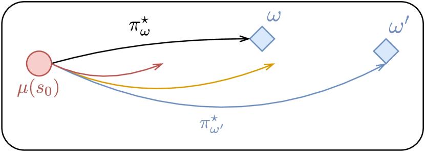
(a) Learning πωsubscriptsuperscript𝜋superscript𝜔\pi^{\star}_{\omega^{\prime}} from scratch
Refer to caption
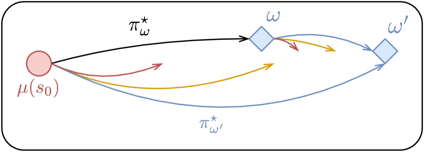
(b) Learning πωsubscriptsuperscript𝜋superscript𝜔\pi^{\star}_{\omega^{\prime}} with Rollin
Figure 1: Illustration of Rollin. The red circle represents the initial state distribution. The dark curve represents the optimal policy of the preceding task ω𝜔\omega. The blue diamonds represent the optimal state distributions dμπω,dμπωsuperscriptsubscript𝑑𝜇superscriptsubscript𝜋𝜔superscriptsubscript𝑑𝜇superscriptsubscript𝜋superscript𝜔d_{\mu}^{\pi_{\omega}^{\star}},d_{\mu}^{\pi_{\omega^{\prime}}^{\star}} of the preceding task ω𝜔\omega and the current ωsuperscript𝜔\omega^{\prime} respectively. Rollin runs the optimal policy of the preceding task πωsubscriptsuperscript𝜋𝜔\pi^{\star}_{\omega} to obtain a better initial state distribution for faster learning of the optimal policy of the current task πωsubscriptsuperscript𝜋superscript𝜔\pi^{\star}_{\omega^{\prime}}.

On the other hand, a number of recent works have proposed multi-task learning methods in RL that involve learning contextual policies that simultaneously represent solutions to an entire space of tasks, such as policies that reach any potential goal (Fu et al., 2018; Eysenbach et al., 2020b; Fujita et al., 2020; Zhai et al., 2022), policies conditioned on language commands (Nair et al., 2022), or even policies conditioned on the parameters of parametric reward functions (Kulkarni et al., 2016; Siriwardhana et al., 2019; Eysenbach et al., 2020a; Yu et al., 2020b). While such methods are often not motivated directly from the standpoint of handling challenging exploration scenarios, but rather directly aim to acquire policies that can perform all tasks in the task space, these multi-task formulations often present a more tractable learning problem than acquiring a solution to a single challenging task in the task space (e.g., the hardest goal, or the most complex language command). We pose the following question:

When do we expect solving the reformulated multi-task RL problem with task-conditioned policies to be more efficient than solving the original single-task problem directly?

In this work, we study this question by analyzing the complexity of learning an optimal policy in the stochastic policy gradient (SPG) setting (Agarwal et al., 2021; Mei et al., 2020; Ding et al., 2021) with a curriculum (learning a list of tasks in sequence). As pointed out by Ding et al. (2021), for learning an optimal policy, SPG requires a polynomial sample complexity if the initialization is near-optimal.111See Definition 4.2 of Section 4.2. In general, there is no guarantee that the initial policy is near-optimal, which could potentially lead to an unbounded density ratio and thus poor sample complexity bound. While there have been a lot of prior works that utilize exploration bonuses to address the sample complexity (Azar et al., 2017; Jin et al., 2018; Agarwal et al., 2020; Zhang et al., 2020d), we take a different approach without the need for exploration bonuses by making use of a curriculum of tasks where adjacent tasks in the curriculum are close in terms of their optimal state visitation distributions. Our algorithm, Rollin, works by (1) using the optimal policy parameters of the previous task as an initialization for the current task, and (2) constructing the initial state distribution as a mixture of the optimal state visitation distribution of the previous task and the original initial state distribution of interest. In a nutshell, Rollin mixes in the distribution of the optimal policy of the preceding task to the initial distribution to make sure that such distribution is close to the optimal state visitation distribution of the current task, reducing the density mismatch ratio and yielding better sample complexity.

We illustrate the intuition of Rollin in Figure 1. We adopt the contextual MDP formulation, where we assume each MDP, ωsubscript𝜔\mathcal{M}_{\omega}, is uniquely defined by a context ω𝜔\omega in the context space 𝒲𝒲\mathcal{W}, and we are given a curriculum {ωk}k=0Ksuperscriptsubscriptsubscript𝜔𝑘𝑘0𝐾\{\omega_{k}\}_{k=0}^{K}, with the last MDP, ωKsubscriptsubscript𝜔𝐾\mathcal{M}_{\omega_{K}}, being the MDP of interest. Our main results require a Lipschitz continuity assumption on the context-dependent reward function rωsubscript𝑟𝜔r_{\omega} and a fixed transition dynamics model across all contexts. We show that learning πKsubscriptsuperscript𝜋𝐾\pi^{\star}_{K} by recursively rolling in with a near-optimal policy for ωksubscript𝜔𝑘\omega_{k} to construct the initial distribution μk+1subscript𝜇𝑘1\mu_{k+1} for the next context ωk+1subscript𝜔𝑘1\omega_{k+1}, can have a smaller minimum required sample complexity compared with learning πωKsubscriptsuperscript𝜋subscript𝜔𝐾\pi^{\star}_{\omega_{K}} from scratch directly. In particular, we show that when an appropriate sequence of contexts is selected, we can reduce the minimum required iteration and sample complexity bounds of entropy-regularized softmax policy gradient (with an inexact stochastic estimation of the gradient) from an original exponential dependency on the state space size, as suggested by Ding et al. (2021), to a polynomial dependency. We also prescribe a practical implementation of Rollin.

Our contributions are as follows. We introduce Rollin, a simple algorithm that facilitates single-task learning by recasting it as a multi-task problem. Theoretically, we show that under the entropy-regularized softmax policy gradient (PG) setting, our algorithm reduces the exponential complexity bound to a polynomial dependency on S𝑆S. Empirically, we verify our theory on a tabular MDP and provide a practical implementation of Rollin that can accelerate curriculum learning in the tabular environment and a range of simulated robotic tasks.

2 Related Work

Convergence of policy gradient methods.

Theoretical analysis of policy gradient methods has a long history (Williams, 1992; Sutton et al., 1999; Konda and Tsitsiklis, 1999; Kakade and Langford, 2002; Peters and Schaal, 2008). Motivated by the recent empirical success (Schulman et al., 2015, 2017) in policy gradient (PG) methods, the theory community has extensively studied the convergence of PG in various settings (Fazel et al., 2018; Agarwal et al., 2021, 2020; Bhandari and Russo, 2019; Mei et al., 2020; Zhang et al., 2020b; Agarwal et al., 2020; Zhang et al., 2020a; Li et al., 2021; Cen et al., 2021; Ding et al., 2021; Yuan et al., 2022; Moskovitz et al., 2022). Agarwal et al. (2021) established the asymptotic global convergence of policy gradient under different policy parameterizations. We extend the result of entropy regularized PG with stochastic gradient (Ding et al., 2021) to the contextual MDP setting. In particular, our contextual MDP setting reduces the exponential state space dependency w.r.t. the iteration number and per iteration sample complexity suggested by Ding et al. (2021) to a polynomial dependency. While there exists convergence analyses on other variants of PG that produce an iteration number that does not suffer from an exponential state space dependency (Agarwal et al., 2021; Mei et al., 2020), they assume access to the exact gradient during each update of PG. In contrast, we assume a stochastic estimation of the gradient.

Exploration bonuses.

A number of prior works have shown that one can achieve a polynomial complexity of learning an optimal policy with effective exploration methods (Azar et al., 2017; Jin et al., 2018; Du et al., 2019; Misra et al., 2020; Agarwal et al., 2020; Zhang et al., 2020d). The computational efficiency suggested by our work is different from some of the aforementioned prior methods that rely on adding exploration bonuses (Azar et al., 2017; Jin et al., 2018; Agarwal et al., 2020; Zhang et al., 2020d), as we assume access to a “good” curriculum which ensures the optimal policy of the next context is not too different from the optimal policy of the current context while eschewing exploration bonuses entirely.

Contextual MDPs.

Contextual MDPs (or MDPs with side information) have been studied extensively in the theoretical RL literature (Abbasi-Yadkori and Neu, 2014; Hallak et al., 2015; Dann et al., 2019; Jiang et al., 2017; Modi et al., 2018; Sun et al., 2019; Dann et al., 2019; Modi et al., 2020). We analyze the iteration complexity and sample complexity of (stochastic) policy gradient methods, which is distinct from these prior works that mainly focus on regret bounds (Abbasi-Yadkori and Neu, 2014; Hallak et al., 2015; Dann et al., 2019) and PAC bounds (Jiang et al., 2017; Modi et al., 2018; Sun et al., 2019; Dann et al., 2019; Modi et al., 2020). Several works assumed linear transition kernel and reward model (or generalized linear model (Abbasi-Yadkori and Neu, 2014)) with respect to the context (Abbasi-Yadkori and Neu, 2014; Modi et al., 2018; Dann et al., 2019; Modi et al., 2020; Belogolovsky et al., 2021). These assumptions share similarity to our assumptions — we have a weaker Lipschitz continuity assumption with respect to the context space (since linear implies Lipschitz) on the reward function and a stronger shared transition kernel assumption.

Curriculum learning in reinforcement learning.

Curriculum learning is a powerful idea that has been widely used in RL (Florensa et al., 2017; Kim and Choi, 2018; Omidshafiei et al., 2019; Ivanovic et al., 2019; Akkaya et al., 2019; Portelas et al., 2020; Bassich et al., 2020; Fang et al., 2020; Klink et al., 2020; Dennis et al., 2020; Parker-Holder et al., 2022; Liu et al., 2022) (also see (Narvekar et al., 2020) for a detailed survey). Although curricula formed by well-designed reward functions (Vinyals et al., 2019; OpenAI, 2018; Berner et al., 2019; Ye et al., 2020; Zhai et al., 2022) are usually sufficient given enough domain knowledge, tackling problems with limited domain knowledge requires a more general approach where a suitable curriculum is automatically formed from a task space. In the goal-conditioned reinforcement learning literature, this corresponds to automatic goal proposal mechanisms (Florensa et al., 2018; Warde-Farley et al., 2018; Sukhbaatar et al., 2018; Ren et al., 2019; Ecoffet et al., 2019; Hartikainen et al., 2019; Pitis et al., 2020; Zhang et al., 2020c; OpenAI et al., 2021; Zhang et al., 2021). The practical instantiation of this work is also similar to (Bassich et al., 2020; Liu et al., 2022), where a curriculum is adopted for learning a progression of a set of tasks. Klink et al. (2022) also analyzed the theoretical benefits of curriculum learning in RL, but is primarily concerned with the problem of representations for value functions when utilizing approximate value iteration methods for curriculum learning. This is accomplished by using boosting to increase the effective capacity of the value function estimator. In contrast, our method does not make any prescription in regard to the representation, but is aimed at studying sample complexity and exploration, showing that "rolling in" with the previous policy and then collecting data with the new policy leads to good sample complexity. In principle, we could even imagine in future work combining the representation analysis in Klink et al. (2022) with the discussion of state coverage in our analysis.

Learning conditional policies in multi-task RL.

Multi-task RL (Tanaka and Yamamura, 2003) approaches usually learn a task-conditioned policy that is shared across different tasks (Rusu et al., 2015; Rajeswaran et al., 2016; Andreas et al., 2017; Finn et al., 2017; D’Eramo et al., 2020; Yu et al., 2020a; Ghosh et al., 2021; Kalashnikov et al., 2021; Agarwal et al., 2022). Compared to learning each task independently, joint training enjoys the sample efficiency benefits from sharing the learned experience across different tasks as long as the policies generalize well across tasks. To encourage generalization, it is often desirable to condition policies on low dimensional feature representations that are shared across different tasks instead (e.g., using variational auto-encoders (Nair et al., 2018; Pong et al., 2019; Nair et al., 2020) or variational information bottleneck (Goyal et al., 2019, 2020; Mendonca et al., 2021)). The idea of learning contextual policies has also been discussed in classical adaptive control literature (Sastry et al., 1990; Tao, 2003; Landau et al., 2011; Åström and Wittenmark, 2013; Goodwin and Sin, 2014). Different from these prior works which have been mostly focusing on learning policies that can generalize across different tasks, our work focuses on how the near-optimal policy from a learned task could be used to help the learning of a similar task.

3 Preliminaries

We consider the contextual MDP setting, where a contextual MDP, 𝒲=(𝒲,𝒮,𝒜,𝐏,rω,γ,ρ)subscript𝒲𝒲𝒮𝒜𝐏subscript𝑟𝜔𝛾𝜌\mathcal{M}_{\mathcal{W}}=(\mathcal{W},\mathcal{S},\mathcal{A},\mathbf{P},r_{\omega},\gamma,\rho), consists of a context space 𝒲𝒲\mathcal{W}, a state space 𝒮𝒮\mathcal{S}, an action space 𝒜𝒜\mathcal{A}, a transition dynamic function 𝐏:𝒮×𝒜𝒫(𝒮):𝐏𝒮𝒜𝒫𝒮\mathbf{P}:\mathcal{S}\times\mathcal{A}\rightarrow\mathcal{P}(\mathcal{S}) (where 𝒫(X)𝒫𝑋\mathcal{P}(X) denotes the set of all probability distributions over set X𝑋X), a context-conditioned reward function r:𝒲×𝒮×𝒜[0,1]:𝑟𝒲𝒮𝒜01r:\mathcal{W}\times\mathcal{S}\times\mathcal{A}\rightarrow[0,1], a discount factor γ(0,1]𝛾01\gamma\in(0,1], and an initial state distribution of interest ρ𝜌\rho. For convenience, we use S=|𝒮|,A=|𝒜|formulae-sequence𝑆𝒮𝐴𝒜S=|\mathcal{S}|,A=|\mathcal{A}| to denote the number of states and actions. While some contextual MDP formulations (Hallak et al., 2015) have context-conditioned transition dynamics and reward functions, we consider the setting where only the reward function can change across contexts. We denote rωsubscript𝑟𝜔r_{\omega} as the reward function conditioned on a fixed ω𝒲𝜔𝒲\omega\in\mathcal{W} and ω=(𝒮,𝒜,𝐏,rω,γ,ρ)subscript𝜔𝒮𝒜𝐏subscript𝑟𝜔𝛾𝜌\mathcal{M}_{\omega}=(\mathcal{S},\mathcal{A},\mathbf{P},r_{\omega},\gamma,\rho) as the MDP induced by such fixed reward function. We use π(a|s):𝒮𝒫(𝒜):𝜋conditional𝑎𝑠𝒮𝒫𝒜\pi(a|s):\mathcal{S}\rightarrow\mathcal{P}(\mathcal{A}) to denote a policy and we adopt the softmax parameterization: πθ(a|s)=exp[θ(s,a)]aexp[θ(s,a)]subscript𝜋𝜃conditional𝑎𝑠𝜃𝑠𝑎subscriptsuperscript𝑎𝜃𝑠superscript𝑎{\pi_{\theta}(a|s)=\frac{\exp\left[\theta(s,a)\right]}{\sum_{a^{\prime}}\exp\left[\theta(s,a^{\prime})\right]}}, where θ:𝒮×𝒜:𝜃maps-to𝒮𝒜{\theta:\mathcal{S}\times\mathcal{A}\mapsto\mathbb{R}}. We use dρπ(s):=(1γ)t=0γtπ(st=s|s0ρ)assignsubscriptsuperscript𝑑𝜋𝜌𝑠1𝛾superscriptsubscript𝑡0superscript𝛾𝑡superscript𝜋subscript𝑠𝑡conditional𝑠subscript𝑠0similar-to𝜌d^{\pi}_{\rho}(s):=(1-\gamma)\sum_{t=0}^{\infty}\gamma^{t}\mathbb{P}^{\pi}(s_{t}=s|s_{0}\sim\rho) to denote the discounted state visitation distribution and Vωπ:=𝔼[t=0γtrω(st,at)]+α(ρ,π)assignsubscriptsuperscript𝑉𝜋𝜔𝔼delimited-[]superscriptsubscript𝑡0superscript𝛾𝑡subscript𝑟𝜔subscript𝑠𝑡subscript𝑎𝑡𝛼𝜌𝜋{V^{\pi}_{\omega}:=\mathbb{E}\left[\sum_{t=0}^{\infty}\gamma^{t}r_{\omega}(s_{t},a_{t})\right]+\alpha\mathbb{H}(\rho,\pi)} to denote the entropy regularized discounted return on ωsubscript𝜔\mathcal{M}_{\omega}, where (ρ,π):=𝔼s0ρ,ahπ(|sh)[h=0γhlogπ(ah|sh)]\mathbb{H}(\rho,\pi):={\mathbb{E}}_{s_{0}\sim\rho,a_{h}\sim\pi(\cdot|s_{h})}\left[\sum_{h=0}^{\infty}-\gamma^{h}\log\pi(a_{h}|s_{h})\right] is the discounted entropy term. We use πω:=argmaxπVωπassignsubscriptsuperscript𝜋𝜔subscript𝜋subscriptsuperscript𝑉𝜋𝜔\pi^{\star}_{\omega}:=\arg\max_{\pi}V^{\pi}_{\omega} to denote an optimal policy that maximizes the discounted return under ωsubscript𝜔\mathcal{M}_{\omega}. We assume all the contextual reward functions are bounded within [0,1]01[0,1]: rω(s,a)[0,1],ω𝒲,(s,a)𝒮×𝒜formulae-sequencesubscript𝑟𝜔𝑠𝑎01formulae-sequencefor-all𝜔𝒲for-all𝑠𝑎𝒮𝒜r_{\omega}(s,a)\in[0,1],\;\forall\omega\in\mathcal{W},\forall(s,a)\in\mathcal{S}\times\mathcal{A}. Similarly to previous analysis (Agarwal et al., 2021; Mei et al., 2020; Ding et al., 2021), we assume the initial distribution ρ𝜌\rho for PG or stochastic PG satisfies ρ(s)>0,s𝒮formulae-sequence𝜌𝑠0for-all𝑠𝒮\rho(s)>0,\forall s\in\mathcal{S}. Supposing we are given a curriculum {ωk}k=0Ksuperscriptsubscriptsubscript𝜔𝑘𝑘0𝐾\{\omega_{k}\}_{k=0}^{K}, where the last context ωKsubscript𝜔𝐾\omega_{K} defines ωKsubscriptsubscript𝜔𝐾\mathcal{M}_{\omega_{K}} the MDP of interest, our goal is to show that sequentially solving πωksuperscriptsubscript𝜋subscript𝜔𝑘\pi_{\omega_{k}}^{\star} for k=0,1,,K𝑘01𝐾k=0,1,\dots,K, enjoys better computational complexity and sample complexity than learning πωKsubscriptsuperscript𝜋subscript𝜔𝐾\pi^{\star}_{\omega_{K}} problem ωKsubscriptsubscript𝜔𝐾\mathcal{M}_{\omega_{K}} from scratch.

3.1 Assumptions

As we will show in Section 4, if there is a curriculum {ωk}k=0Ksuperscriptsubscriptsubscript𝜔𝑘𝑘0𝐾\{\omega_{k}\}_{k=0}^{K} where the optimal policies πωk,πωk+1subscriptsuperscript𝜋subscript𝜔𝑘subscriptsuperscript𝜋subscript𝜔𝑘1\pi^{\star}_{\omega_{k}},\pi^{\star}_{\omega_{k+1}} with respect to two consecutive contexts ωk,ωk+1subscript𝜔𝑘subscript𝜔𝑘1\omega_{k},\omega_{k+1} are close enough to each other in terms of their state visitation distributions, using an ε𝜀\varepsilon-optimal policy of ωksubscript𝜔𝑘\omega_{k} as an initialization allows us to directly start from the near-optimal regime of ωk+1subscript𝜔𝑘1\omega_{k+1}, hence only requiring polynomial complexity to learn πωk+1subscriptsuperscript𝜋subscript𝜔𝑘1\pi^{\star}_{\omega_{k+1}}. We describe our curriculum assumptions as follows.

Assumption 3.1 (Lipschitz reward in the context space).

The reward function is Lipschitz continuous with respect to the context: maxs,a|rω(s,a)rω(s,a)|Lrωω2subscript𝑠𝑎subscript𝑟𝜔𝑠𝑎subscript𝑟superscript𝜔𝑠𝑎subscript𝐿𝑟subscriptnorm𝜔superscript𝜔2\max_{s,a}\left|r_{\omega}(s,a)-r_{\omega^{\prime}}(s,a)\right|\leq L_{r}\left\|\omega-\omega^{\prime}\right\|_{2}, ω,ω𝒲for-all𝜔superscript𝜔𝒲\forall\omega,\omega^{\prime}\in\mathcal{W}.

Intuitively, 3.1 defines the similarity between two tasks via a Lipschitz continuity in the context space. Similar Lipschitz assumptions also appears in (Abbasi-Yadkori and Neu, 2014; Modi et al., 2018; Dann et al., 2019; Modi et al., 2020; Belogolovsky et al., 2021).

Assumption 3.2 (Similarity of Two Contexts).

The curriculum {ωk}k=0Ksuperscriptsubscriptsubscript𝜔𝑘𝑘0𝐾\{\omega_{k}\}_{k=0}^{K} satisfies max0kK1ωk+1ωk2O(S2)subscript0𝑘𝐾1subscriptnormsubscript𝜔𝑘1subscript𝜔𝑘2𝑂superscript𝑆2\max_{0\leq k\leq K-1}\left\|\omega_{k+1}-\omega_{k}\right\|_{2}\leq O\left(S^{-2}\right), and we have access to a near-optimal initialization θ0(0)superscriptsubscript𝜃00\theta_{0}^{(0)} for learning πω0subscriptsuperscript𝜋subscript𝜔0\pi^{\star}_{\omega_{0}} (formally defined in Section 4.2).

At first glance, the near-optimal initialization θ0(0)superscriptsubscript𝜃00\theta_{0}^{(0)} for the first task ω0subscript𝜔0\omega_{0} in the curriculum (suggested by 3.2) may seem like a strong assumption, but in many practical settings, it could be quite easy to obtain. For example, if the tasks correspond to reaching different goals, the curriculum might start with a goal right on top of the starting state, and therefore trivially easy to learn. As another example, if the task is a locomotion task and ω𝜔\omega contexts correspond to target velocities, ω0subscript𝜔0\omega_{0} might correspond to a velocity of zero, corresponding to standing still.

3.1 and 3.2 together quantify the maximum difference between two consecutive tasks ωk1,ωksubscriptsubscript𝜔𝑘1subscriptsubscript𝜔𝑘\mathcal{M}_{\omega_{k-1}},\mathcal{M}_{\omega_{k}}, in terms of the maximum difference between their reward function, which plays a crucial role in reducing the exponential complexity to a polynomial one. We will briefly discuss intuition in the next section.

3.2 Prior Analysis on PG with stochastic gradient

Ding et al. (2021) proposed a two-phased PG convergence analysis framework with a stochastic gradient. In particular, the author demonstrates that with high probability, stochastic PG with arbitrary initialization achieves an ε𝜀\varepsilon-optimal policy can be achieved with iteration numbers of T1,T2subscript𝑇1subscript𝑇2T_{1},T_{2} and per iteration sample complexities of B1,B2subscript𝐵1subscript𝐵2B_{1},B_{2} in two separate phases where T1=Ω~(S2S3),T2=Ω~(S3/2)formulae-sequencesubscript𝑇1~Ωsuperscript𝑆2superscript𝑆3subscript𝑇2~Ωsuperscript𝑆32T_{1}=\widetilde{\Omega}\left(S^{2S^{3}}\right),T_{2}=\widetilde{\Omega}\left(S^{3/2}\right) (Ω~()~Ω\widetilde{\Omega}(\cdot) suppresses the logS𝑆\log S and terms that do not contain S𝑆S) and B1=Ω~(S2S3),B2=Ω~(S5)formulae-sequencesubscript𝐵1~Ωsuperscript𝑆2superscript𝑆3subscript𝐵2~Ωsuperscript𝑆5B_{1}=\widetilde{\Omega}\left(S^{2S^{3}}\right),B_{2}=\widetilde{\Omega}\left(S^{5}\right), respectively, and PG enters phase 2 only when the updating policy becomes ε0subscript𝜀0\varepsilon_{0}-optimal, where ε0subscript𝜀0\varepsilon_{0} is a term depending on S𝑆S (formally defined by (19) in Section A.3). For completeness, we restate the main theorem of Ding et al. (2021) in Theorem A.2, provide the details of such dependencies on S𝑆S in Corollary A.3, and describe the two-phase procedure in Algorithm 4. The main implication of the two-phase results is that, when applying SPG to learn an optimal policy from an arbitrary initialization, we suffer from exponential complexities, unless the initialization is ε0subscript𝜀0\varepsilon_{0}-optimal. We will now discuss how 3.1 and 3.2 enable an ε0subscript𝜀0\varepsilon_{0}-optimal initialization for every ωksubscript𝜔𝑘\omega_{k}, reducing the exponential complexities to polynomial complexities.

4 Theoretical Analysis

In this section, we first introduce Rollin, a simple algorithm that accelerates policy learning under the contextual MDP setup by bootstrapping new context learning with a better initial distribution (Algorithm 1). Then, we provide the total complexity analysis of applying Rollin to stochastic PG for achieving an ε𝜀\varepsilon-optimal policy. Finally, we validate our theoretical results on a tabular MDP.

4.1 Rollin

The theoretical version of Rollin is provided in Algorithm 1. The intuition behind Rollin is that when two consecutive contexts in the curriculum {ωk}k=1Ksuperscriptsubscriptsubscript𝜔𝑘𝑘1𝐾\{\omega_{k}\}_{k=1}^{K} are close, their optimal parameters θωk1,θωksubscriptsuperscript𝜃subscript𝜔𝑘1subscriptsuperscript𝜃subscript𝜔𝑘\theta^{\star}_{\omega_{k-1}},\theta^{\star}_{\omega_{k}} should be close to each other. Let θt(k)superscriptsubscript𝜃𝑡𝑘\theta_{t}^{(k)} denote the parameters at the tthsuperscript𝑡tht^{\text{th}} iteration of stochastic PG for learning θωksubscriptsuperscript𝜃subscript𝜔𝑘\theta^{\star}_{\omega_{k}}. If we initialize θ0(k)superscriptsubscript𝜃0𝑘\theta_{0}^{(k)} as the optimal parameter of the previous context θωk1superscriptsubscript𝜃subscript𝜔𝑘1\theta_{\omega_{k-1}}^{\star} (line 5 in Algorithm 1), and set the initial distribution μksubscript𝜇𝑘\mu_{k} as a mixture of the optimal state visitation distribution of the previous context dμk1πωk1subscriptsuperscript𝑑superscriptsubscript𝜋subscript𝜔𝑘1subscript𝜇𝑘1d^{\pi_{\omega_{k-1}}^{\star}}_{\mu_{k-1}} and the original distribution of interest ρ𝜌\rho with β(0,1)𝛽01\beta\in(0,1) (line 6 in Algorithm 1),

μk=βdμk1πωk1+(1β)ρ,subscript𝜇𝑘𝛽subscriptsuperscript𝑑superscriptsubscript𝜋subscript𝜔𝑘1subscript𝜇𝑘11𝛽𝜌\mu_{k}=\beta d^{\pi_{\omega_{k-1}}^{\star}}_{\mu_{k-1}}+(1-\beta)\rho, (1)

then we can show that stochastic PG enjoys a faster convergence rate. This is because setting θ0(k)=θk1superscriptsubscript𝜃0𝑘subscriptsuperscript𝜃𝑘1\theta_{0}^{(k)}=\theta^{\star}_{k-1} ensures a near-optimal initialization for learning ωksubscript𝜔𝑘\omega_{k}, and setting μksubscript𝜇𝑘\mu_{k} as the mixture further improves the rate of convergence by decreasing the density mismatch ratio dμkπωk/μksubscriptnormsubscriptsuperscript𝑑subscriptsuperscript𝜋subscript𝜔𝑘subscript𝜇𝑘subscript𝜇𝑘\Big{\|}d^{\pi^{\star}_{\omega_{k}}}_{\mu_{k}}/\mu_{k}\Big{\|}_{\infty} (a term with that influences the convergence rate).

4.2 Main Results

We now discuss how to use a sequence of contexts to learn the target context ωKsubscript𝜔𝐾\omega_{K} with provable efficiency given a near-optimal policy πθ0(0)subscript𝜋subscriptsuperscript𝜃00\pi_{\theta^{(0)}_{0}} of the initial context ω0subscript𝜔0\omega_{0}, without incurring an exponential dependency on S𝑆S (as mentioned in Section 3.2). Our polynomial complexity comes as a result of enforcing an ε0subscript𝜀0\varepsilon_{0}-optimal initialization (ε0subscript𝜀0\varepsilon_{0} is the same as Section 3.2 and (19)) for running stochastic PG (line 6 of Algorithm 1). Hence, stochastic PG directly enters phase 2, with a polynomial dependency on S𝑆S.

Our main results consist of two parts. We first show that when two consecutive contexts ωk1,ωksubscript𝜔𝑘1subscript𝜔𝑘\omega_{k-1},\omega_{k} are close enough to each other, using Rollin for learning θksubscriptsuperscript𝜃𝑘\theta^{\star}_{k} with initialization θ0(k)=θωk1superscriptsubscript𝜃0𝑘subscriptsuperscript𝜃subscript𝜔𝑘1\theta_{0}^{(k)}=\theta^{\star}_{\omega_{k-1}} and applying an initial distribution μk=βdμk1πωk1+(1β)ρsubscript𝜇𝑘𝛽subscriptsuperscript𝑑superscriptsubscript𝜋subscript𝜔𝑘1subscript𝜇𝑘11𝛽𝜌\mu_{k}=\beta d^{\pi_{\omega_{k-1}}^{\star}}_{\mu_{k-1}}+(1-\beta)\rho improves the convergence rate. Specifically, the iteration number and complexity for learning θωksubscriptsuperscript𝜃subscript𝜔𝑘\theta^{\star}_{\omega_{k}} from θωk1subscriptsuperscript𝜃subscript𝜔𝑘1\theta^{\star}_{\omega_{k-1}} are stated as follows:

Algorithm 1 Provably Efficient Learning via Rollin
1:Input: ρ𝜌\rho, {ωk}k=0Ksuperscriptsubscriptsubscript𝜔𝑘𝑘0𝐾\{\omega_{k}\}_{k=0}^{K}, 𝒲subscript𝒲\mathcal{M}_{\mathcal{W}}, β(0,1)𝛽01\beta\in(0,1), θ0(0)subscriptsuperscript𝜃00\theta^{(0)}_{0}.
2:Initialize μ0=ρsubscript𝜇0𝜌\mu_{0}=\rho.
3:Run stochastic PG (Algorithm 4) with initialization θ0(0)superscriptsubscript𝜃00\theta_{0}^{(0)}, μ0,ω0subscript𝜇0subscriptsubscript𝜔0\mu_{0},\mathcal{M}_{\omega_{0}} and obtain θω0subscriptsuperscript𝜃subscript𝜔0\theta^{\star}_{\omega_{0}}.
4:for k=1,,K𝑘1𝐾k=1,\dots,K do
5:      Set θ1(k)=θωk1subscriptsuperscript𝜃𝑘1subscriptsuperscript𝜃subscript𝜔𝑘1\theta^{(k)}_{1}=\theta^{\star}_{\omega_{k-1}}.\triangleright πθωk1subscript𝜋subscriptsuperscript𝜃subscript𝜔𝑘1\pi_{\theta^{\star}_{\omega_{k-1}}} is optimal for ωk1subscript𝜔𝑘1\omega_{k-1}.
6:      Set μk=βdμk1πωk1+(1β)ρsubscript𝜇𝑘𝛽subscriptsuperscript𝑑superscriptsubscript𝜋subscript𝜔𝑘1subscript𝜇𝑘11𝛽𝜌\mu_{k}=\beta d^{\pi_{\omega_{k-1}}^{\star}}_{\mu_{k-1}}+(1-\beta)\rho.
7:     Run stochastic PG (Algorithm 4) with initialization θ0(k)superscriptsubscript𝜃0𝑘\theta_{0}^{(k)}, μk,ωksubscript𝜇𝑘subscriptsubscript𝜔𝑘\mu_{k},\mathcal{M}_{\omega_{k}} and obtain θωksubscriptsuperscript𝜃subscript𝜔𝑘\theta^{\star}_{\omega_{k}}.
8:end for
9:Output: θωKsuperscriptsubscript𝜃subscript𝜔𝐾\theta_{\omega_{K}}^{\star}
Entropy Coeff. Baseline Rollin
Hard α=0.01𝛼0.01\alpha=0.01 0.500±0.000plus-or-minus0.5000.0000.500\pm 0.000 0.562±0.000plus-or-minus0.5620.0000.562\pm 0.000
α=0.001𝛼0.001\alpha=0.001 0.856±0.006plus-or-minus0.8560.0060.856\pm 0.006 1.000±0.000plus-or-minus1.0000.0001.000\pm 0.000
Easy α=0.01𝛼0.01\alpha=0.01 0.944±0.003plus-or-minus0.9440.0030.944\pm 0.003 1.000±0.000plus-or-minus1.0000.0001.000\pm 0.000
α=0.001𝛼0.001\alpha=0.001 1.000±0.000plus-or-minus1.0000.0001.000\pm 0.000 1.000±0.000plus-or-minus1.0000.0001.000\pm 0.000
Entropy Coeff. Baseline Rollin
Hard α=0.01𝛼0.01\alpha=0.01 0.000±0.000plus-or-minus0.0000.0000.000\pm 0.000 0.000±0.000plus-or-minus0.0000.0000.000\pm 0.000
α=0.001𝛼0.001\alpha=0.001 0.424±0.023plus-or-minus0.4240.0230.424\pm 0.023 1.067±0.000plus-or-minus1.0670.0001.067\pm 0.000
Easy α=0.01𝛼0.01\alpha=0.01 4.093±0.224plus-or-minus4.0930.2244.093\pm 0.224 7.374±0.216plus-or-minus7.3740.2167.374\pm 0.216
α=0.001𝛼0.001\alpha=0.001 10.536±0.002plus-or-minus10.5360.00210.536\pm 0.002 10.620±0.002plus-or-minus10.6200.00210.620\pm 0.002
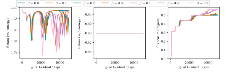
Table 1: Curriculum progress κ𝜅\kappa (left) and final return Vπsuperscript𝑉𝜋V^{\pi} (right) on the four-room navigation with stochastic PG. Both metrics are reported at the 50,000th50superscript000th50,000^{\text{th}} gradient step. We use a mixing ratio of β=0.75𝛽0.75\beta=0.75. Across two entropy coefficients and two reward settings (easy and hard), stochastic PG with Rollin consistently achieves better curriculum progress and final return. The standard error is computed over 10 random seeds.
Theorem 4.1 (Complexity of Learning the Next Context).

Consider the context-based stochastic softmax policy gradient (line 7 of Algorithm 1), and suppose 3.1 and 3.2 hold, then the iteration number of obtaining an ε𝜀\varepsilon-optimal policy for ωksubscript𝜔𝑘\omega_{k} from θωk1subscriptsuperscript𝜃subscript𝜔𝑘1\theta^{\star}_{\omega_{k-1}} is Ω~(S)~Ω𝑆\widetilde{\Omega}\left(S\right) and the per iteration sample complexity is Ω~(Lrα(1β)S3)~Ωsubscript𝐿𝑟𝛼1𝛽superscript𝑆3\widetilde{\Omega}\left(\frac{L_{r}}{\alpha(1-\beta)}S^{3}\right).

Theorem 4.1 shows that when ωk1,ωksubscript𝜔𝑘1subscript𝜔𝑘\omega_{k-1},\omega_{k} are close enough, Rollin reduces the minimum required iteration and sample complexity from an exponential dependency of Ω~(S2S3)~Ωsuperscript𝑆2superscript𝑆3\widetilde{\Omega}(S^{2S^{3}}) to an iteration number of Ω~(S)~Ω𝑆\widetilde{\Omega}(S) and per iteration sample complexity of Ω~(S3)~Ωsuperscript𝑆3\widetilde{\Omega}(S^{3}). It is worth noting that the theorem above only addresses the iteration number and sample complexity for learning θωksubscriptsuperscript𝜃subscript𝜔𝑘\theta^{\star}_{\omega_{k}} from θωk1subscriptsuperscript𝜃subscript𝜔𝑘1\theta^{\star}_{\omega_{k-1}}. Theorem 4.3 provides the total complexity for learning θωKsuperscriptsubscript𝜃subscript𝜔𝐾\theta_{\omega_{K}}^{\star} from θ0(0)superscriptsubscript𝜃00\theta_{0}^{(0)} via recursively applying the results in Theorem 4.1. Before introducing Theorem 4.3, we first provide a criterion for the desired initialization of θ0(0)superscriptsubscript𝜃00\theta_{0}^{(0)}.

Definition 4.2 (Near-optimal Initialization).

We say θ0subscript𝜃0\theta_{0} is a near-optimal initialization for learning θωsuperscriptsubscript𝜃𝜔\theta_{\omega}^{\star} if θ0subscript𝜃0\theta_{0} satisfies Vωπω(ρ)Vωπθ0(ρ)<ε0subscriptsuperscript𝑉subscriptsuperscript𝜋𝜔𝜔𝜌subscriptsuperscript𝑉subscript𝜋subscript𝜃0𝜔𝜌subscript𝜀0V^{\pi^{\star}_{\omega}}_{\omega}(\rho)-V^{\pi_{\theta_{0}}}_{\omega}(\rho)<\varepsilon_{0} and ρdρπω01ω1ω02subscriptnorm𝜌superscriptsubscript𝑑𝜌subscriptsuperscript𝜋subscript𝜔01subscriptnormsubscript𝜔1subscript𝜔02\left\|\rho-d_{\rho}^{\pi^{\star}_{\omega_{0}}}\right\|_{1}\leq\left\|\omega_{1}-\omega_{0}\right\|_{2}.

Note that in the above definition, πωksubscriptsuperscript𝜋subscript𝜔𝑘\pi^{\star}_{\omega_{k}} represents the optimal policy of ωksubscript𝜔𝑘\omega_{k}, and Vωkπsubscriptsuperscript𝑉𝜋subscript𝜔𝑘V^{\pi}_{\omega_{k}} represents value function of context ωksubscript𝜔𝑘\omega_{k} under policy π𝜋\pi. We now introduce the results for the overall complexity:

Theorem 4.3 (Main Results: Total Complexity of Rollin).

Suppose 3.1 and 3.2 hold, and θ0(0)subscriptsuperscript𝜃00\theta^{(0)}_{0} is a near-optimal initialization, then the total number of iterations of learning πωKsubscriptsuperscript𝜋subscript𝜔𝐾\pi^{\star}_{\omega_{K}} using Algorithm 1 is Ω(KS)Ω𝐾𝑆\Omega(KS) and the per iteration sample complexity is Ω~(S3)~Ωsuperscript𝑆3\widetilde{\Omega}\left(S^{3}\right), with high probability.

A direct implication of Theorem 4.3 is that, with a curriculum {ωk}k=0Ksuperscriptsubscriptsubscript𝜔𝑘𝑘0𝐾\{\omega_{k}\}_{k=0}^{K} satisfying 3.1 and 3.2, one can reduce the daunting exponential dependency on S𝑆S caused by poor initialization to a polynomial dependency. Admittedly the state space S𝑆S itself is still large in practice, but reducing the state space S𝑆S itself requires extra assumptions on 𝒮𝒮\mathcal{S}, which is beyond the scope of this work. We now provide a sketch proof of Theorem 4.1 and Theorem 4.3 in the next subsection and leave all the details to Section A.4 and Section A.5 respectively.

4.3 Proof Sketch

Sketch proof of Theorem 4.1.

The key insight for proving Theorem 4.1 is to show that in MDP ωksubscriptsubscript𝜔𝑘\mathcal{M}_{\omega_{k}}, the value function with respect to πωk,πωk1subscriptsuperscript𝜋subscript𝜔𝑘subscriptsuperscript𝜋subscript𝜔𝑘1\pi^{\star}_{\omega_{k}},\pi^{\star}_{\omega_{k-1}} can be bounded by the 2superscript2\ell^{2}-norm between ωksubscript𝜔𝑘\omega_{k} and ωk1subscript𝜔𝑘1\omega_{k-1}. In particular, we prove such a relation in Lemma A.5:

Vωkπωk(ρ)Vωkπωk1(ρ)2Lrωkωk12(1γ)2.subscriptsuperscript𝑉subscriptsuperscript𝜋subscript𝜔𝑘subscript𝜔𝑘𝜌subscriptsuperscript𝑉subscriptsuperscript𝜋subscript𝜔𝑘1subscript𝜔𝑘𝜌2subscript𝐿𝑟subscriptnormsubscript𝜔𝑘subscript𝜔𝑘12superscript1𝛾2V^{\pi^{\star}_{\omega_{k}}}_{\omega_{k}}(\rho)-V^{\pi^{\star}_{\omega_{k-1}}}_{\omega_{k}}(\rho)\leq\frac{2L_{r}\left\|\omega_{k}-\omega_{k-1}\right\|_{2}}{(1-\gamma)^{2}}.\vspace{-0.15cm} (2)

By setting θ0(k)=θωk1superscriptsubscript𝜃0𝑘subscriptsuperscript𝜃subscript𝜔𝑘1\theta_{0}^{(k)}=\theta^{\star}_{\omega_{k-1}}, Equation (2) directly implies Vωkπωk(ρ)Vθ0(k)(ρ)2Lrωkωk12(1γ)2subscriptsuperscript𝑉subscriptsuperscript𝜋subscript𝜔𝑘subscript𝜔𝑘𝜌superscript𝑉superscriptsubscript𝜃0𝑘𝜌2subscript𝐿𝑟subscriptnormsubscript𝜔𝑘subscript𝜔𝑘12superscript1𝛾2V^{\pi^{\star}_{\omega_{k}}}_{\omega_{k}}(\rho)-V^{\theta_{0}^{(k)}}(\rho)\leq\frac{2L_{r}\left\|\omega_{k}-\omega_{k-1}\right\|_{2}}{(1-\gamma)^{2}}. As suggested by Ding et al. (2021) stochastic PG can directly start from stage 2 with polynomial complexity of T2=Ω~(S),B2=Ω~(S5)formulae-sequencesubscript𝑇2~Ω𝑆subscript𝐵2~Ωsuperscript𝑆5T_{2}=\widetilde{\Omega}(S),B_{2}=\widetilde{\Omega}(S^{5}), if Vωkπωk(ρ)Vθ0(k)(ρ)ε0subscriptsuperscript𝑉subscriptsuperscript𝜋subscript𝜔𝑘subscript𝜔𝑘𝜌superscript𝑉superscriptsubscript𝜃0𝑘𝜌subscript𝜀0V^{\pi^{\star}_{\omega_{k}}}_{\omega_{k}}(\rho)-V^{\theta_{0}^{(k)}}(\rho)\leq\varepsilon_{0}, where ε0subscript𝜀0\varepsilon_{0} (formally defined in Equation (19) in Section A.3) is a constant satisfying ε0=O(S2)subscript𝜀0𝑂superscript𝑆2\varepsilon_{0}=O(S^{-2}). Hence, by enforcing two consecutive contexts to be close enough ωkωk12O(S2)subscriptnormsubscript𝜔𝑘subscript𝜔𝑘12𝑂superscript𝑆2\left\|\omega_{k}-\omega_{k-1}\right\|_{2}\leq O(S^{-2}), we can directly start from a near-optimal initialization with polynomial complexity with respect to S𝑆S. It is worth highlighting that the per iteration sample complexity B2subscript𝐵2B_{2} shown by Ding et al. (2021) scales as Ω~(S5)~Ωsuperscript𝑆5\widetilde{\Omega}(S^{5}), while our result in Theorem 4.1 only requires a smaller sample complexity of Ω~(S3)~Ωsuperscript𝑆3\widetilde{\Omega}(S^{3}). Such an improvement in the sample complexity comes from line 6 of Rollin: μk=βdμk1πωk1+(1β)ρsubscript𝜇𝑘𝛽subscriptsuperscript𝑑superscriptsubscript𝜋subscript𝜔𝑘1subscript𝜇𝑘11𝛽𝜌\mu_{k}=\beta d^{\pi_{\omega_{k-1}}^{\star}}_{\mu_{k-1}}+(1-\beta)\rho. Intuitively, setting μksubscript𝜇𝑘\mu_{k} as βdμk1πωk1+(1β)ρ𝛽subscriptsuperscript𝑑superscriptsubscript𝜋subscript𝜔𝑘1subscript𝜇𝑘11𝛽𝜌\beta d^{\pi_{\omega_{k-1}}^{\star}}_{\mu_{k-1}}+(1-\beta)\rho allows us to provide an upper bound on the density mismatch ratio:

dμkπμk/μkO~(Lrα(1β)ΔωkS),subscriptnormsubscriptsuperscript𝑑subscriptsuperscript𝜋subscript𝜇𝑘subscript𝜇𝑘subscript𝜇𝑘~𝑂subscript𝐿𝑟𝛼1𝛽subscriptsuperscriptΔ𝑘𝜔𝑆\left\|d^{\pi^{\star}_{\mu_{k}}}_{\mu_{k}}/\mu_{k}\right\|_{\infty}\leq\widetilde{O}\left(\frac{L_{r}}{\alpha(1-\beta)}\Delta^{k}_{\omega}S\right), (3)

where Δωk=max1ikωiωi12superscriptsubscriptΔ𝜔𝑘subscript1𝑖𝑘subscriptnormsubscript𝜔𝑖subscript𝜔𝑖12\Delta_{\omega}^{k}=\max_{1\leq i\leq k}\left\|\omega_{i}-\omega_{i-1}\right\|_{2}. Since the sample complexity B2subscript𝐵2B_{2} (provided in Corollary A.3) contains one multiplier of dμkπμk/μksubscriptnormsubscriptsuperscript𝑑subscriptsuperscript𝜋subscript𝜇𝑘subscript𝜇𝑘subscript𝜇𝑘\left\|d^{\pi^{\star}_{\mu_{k}}}_{\mu_{k}}/\mu_{k}\right\|_{\infty}, setting Δωk=O(S2)superscriptsubscriptΔ𝜔𝑘𝑂superscript𝑆2\Delta_{\omega}^{k}=O(S^{-2}) immediately reduces the complexity by an order of S2superscript𝑆2S^{2}. The proof of the upper bound of the density mismatch ratio (Equation (3)) is provided in Lemma A.1.

Sketch proof of Theorem 4.3.

We obtain Theorem 4.3 by recursively applying Theorem 4.1. More precisely, we use induction to show that, if we initialize the parameters of the policy as θ0(k)=θωk1superscriptsubscript𝜃0𝑘subscriptsuperscript𝜃subscript𝜔𝑘1\theta_{0}^{(k)}=\theta^{\star}_{\omega_{k-1}}, when t=Ω~(S)𝑡~Ω𝑆t=\widetilde{\Omega}(S), k[K]for-all𝑘delimited-[]𝐾\forall k\in[K], we have Vωkπωk(ρ)Vωkπθt(k1)(ρ)<ε0subscriptsuperscript𝑉subscriptsuperscript𝜋subscript𝜔𝑘subscript𝜔𝑘𝜌subscriptsuperscript𝑉subscript𝜋superscriptsubscript𝜃𝑡𝑘1subscript𝜔𝑘𝜌subscript𝜀0V^{\pi^{\star}_{\omega_{k}}}_{\omega_{k}}(\rho)-V^{\pi_{\theta_{t}^{(k-1)}}}_{\omega_{k}}(\rho)<\varepsilon_{0}. Hence, for any context ωk,k[K]subscript𝜔𝑘𝑘delimited-[]𝐾\omega_{k},k\in[K], initializing θ0(k)=θt(k1)superscriptsubscript𝜃0𝑘superscriptsubscript𝜃𝑡𝑘1\theta_{0}^{(k)}=\theta_{t}^{(k-1)} from learning πωk1subscriptsuperscript𝜋subscript𝜔𝑘1\pi^{\star}_{\omega_{k-1}} via stochastic PG after t=Ω(S)𝑡Ω𝑆t=\Omega(S) iteration, θ0(k)superscriptsubscript𝜃0𝑘\theta_{0}^{(k)} will directly start from the efficient phase 2 with polynomial complexity. Hence, the total iteration number for learning the θKsuperscriptsubscript𝜃𝐾\theta_{K}^{\star} is Ω(KS)Ω𝐾𝑆\Omega(KS), and the per iteration sample complexity remains the same as Theorem 4.1 (Ω~(S3)~Ωsuperscript𝑆3\widetilde{\Omega}\left(S^{3}\right)).

Refer to caption
Refer to caption
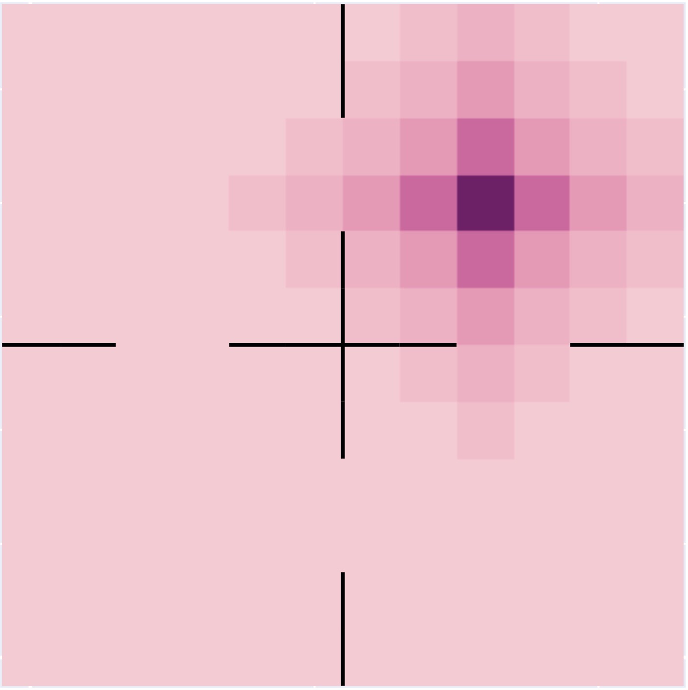
Figure 2: Visualization of the two reward functions for the four-room navigation environment. Left: easy; Right: hard. Darker color indicates a higher reward when the agent reaches the state (with the goal state the darkest). The agent receives 00 reward when it is too far from the goal location (5 steps for the easy reward function and 4 steps for the hard reward function). The black line indicates walls in the environment where the agent cannot pass through. The reward function visualization in this figure is for the last context. The reward function for other contexts (other goals) is the same but with the reward function shifted according to the goal state.

4.4 Numerical Experiments: Four-room Navigation

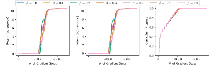
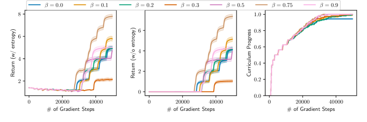
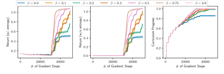
To provide empirical support for the validity of our theoretical results, we follow the exact setting that is used in our theoretical analysis and implement Rollin with stochastic PG and the softmax policy parameterization on a tabular contextual MDP. It is worth highlighting that this is distinct from the practical implementation of Rollin in Section 5 – the focus there is to apply the idea of Rollin to design a sample-efficient deep RL algorithm for a more practical setting (e.g., continuous state and action space), whereas the focus here is solely to validate our theory in the theoretical setting. The contextual MDP is a grid world consisting of 12×12121212\times 12 grid cells where each cell corresponds to a state in the MDP. The agent always starts from the bottom-left corner of the grid world and navigates around to collect rewards. In particular, the agent receives a positive reward when it is close to a pre-defined goal cell/state which is defined by the context. We use a curriculum consisting of 171717 contexts/goals in sequence, {ωk}k=016superscriptsubscriptsubscript𝜔𝑘𝑘016\{\omega_{k}\}_{k=0}^{16}, which form a path from the initial state of the agent to a far away goal location, and we switch from the current context to the next one in the curriculum whenever the current goal location is reached with more than 50%percent5050\% probability. We experiment with two different reward functions (visualized in Figure 2). Table 1 summarizes the results of our experiments. Rollin is able to consistently improve upon the vanilla stochastic PG baseline (across two different entropy coefficients and two reward functions with varying difficulties) in terms of the curriculum progress and the final return. This verifies that Rollin can indeed improve the sample complexity of stochastic PG in a curriculum learning setting, validating our theory. See more implementation details of the numerical experiments in Appendix F.

5 Practical Implementation of Rollin

We have shown empirical evidence through numerical experiments that Rollin can lead to sample complexity reduction under our theoretical setting (tabular MDP with discrete action space and state space, softmax parameterization and entropy regularized objective). Now, we introduce a practical implementation of Rollin using Soft-Actor-Critic (Haarnoja et al., 2018) such that Rollin can be applied to more practical problems with continuous action space and state space. SAC can be seen as a variant of entropy-regularized stochastic PG with the addition of the critics to reduce gradient variance. Recall that in the theoretical analysis, we learn a separate policy for each context that can start from the near-optimal state distribution of the previous context to achieve a good return under the current context. However, in practice, we usually would want to have a policy that can directly start from the initial distribution ρ𝜌\rho to obtain a good return for the final context ωKsubscript𝜔𝐾\omega_{K}. In order to learn such a policy, we propose to have two context-conditioned RL agents training in parallel, where the first agent πmainsubscript𝜋main\pi_{\mathrm{main}} is the main agent that eventually will learn to achieve a good return from ρ𝜌\rho, and the second agent πexpsubscript𝜋exp\pi_{\mathrm{exp}} is an exploration agent that learns to achieve a good return under the current context from the near-optimal state density of the previous context. Another purpose of the exploration agent (as the name suggests) is to provide a better exploration experience for the main agent to learn the current context better. This is made convenient by using an off-policy RL agent where the main agent can learn from the data collected by the exploration agent.

Specifically, for each episode, there is a probability of β𝛽\beta where we run the main agent conditioned on the previous context for a random number of steps until we switch to the exploration agent to collect experience for the current context until the episode ends. Otherwise, we directly run the main agent for the entire episode. Both agents are trained to maximize the return under the current context. Whenever the average return of the last 10 episodes exceeds a performance threshold R𝑅R, we immediately switch to the next context and re-initialize the exploration agent and its replay buffer. A high-level description is available in Algorithm 2 (a more detailed version in Algorithm 8).

Algorithm 2 Practical Implementation of Rollin
1:Input: {ωk}k=0Ksuperscriptsubscriptsubscript𝜔𝑘𝑘0𝐾\{\omega_{k}\}_{k=0}^{K}: input curriculum, R𝑅R: near-optimal threshold, β𝛽\beta: roll-in ratio, H𝐻H: horizon, γ𝛾\gamma: discount factor.
2:Initialize 𝒟,𝒟exp,k0formulae-sequence𝒟formulae-sequencesubscript𝒟exp𝑘0\mathcal{D}\leftarrow\emptyset,\mathcal{D}_{\mathrm{exp}}\leftarrow\emptyset,k\leftarrow 0, and two SAC agents πmainsubscript𝜋main\pi_{\mathrm{main}} and πexpsubscript𝜋exp\pi_{\mathrm{exp}}.
3:for each episode do
4:     if average return of the last 10 episodes under context ωksubscript𝜔𝑘\omega_{k} is greater than R𝑅R  then
5:         kk+1𝑘𝑘1k\leftarrow k+1, 𝒟expsubscript𝒟exp\mathcal{D}_{\mathrm{exp}}\leftarrow\emptyset, and re-initialize the exploration agent πexpsubscript𝜋exp\pi_{\mathrm{exp}}
6:     end if
7:     if k>0𝑘0k>0 and with probability of β𝛽\beta then
8:         hGeom(1γ)similar-toGeom1𝛾h\sim\mathrm{Geom}(1-\gamma) (truncated at H𝐻H)
9:         run πmain(a|s,ωk1)subscript𝜋mainconditional𝑎𝑠subscript𝜔𝑘1\pi_{\mathrm{main}}(a|s,\omega_{k-1}) from the initial state for hh steps and switch to πexp(a|s,ωk)subscript𝜋expconditional𝑎𝑠subscript𝜔𝑘\pi_{\mathrm{exp}}(a|s,\omega_{k}) until the episode ends to obtain trajectory τ0:H={s0,a0,r0,s1,a1,,sH}subscript𝜏:0𝐻subscript𝑠0subscript𝑎0subscript𝑟0subscript𝑠1subscript𝑎1subscript𝑠𝐻\tau_{0:H}=\{s_{0},a_{0},r_{0},s_{1},a_{1},\cdots,s_{H}\}.
10:         record τ0:Hsubscript𝜏:0𝐻\tau_{0:H} in 𝒟𝒟\mathcal{D}, and τh:Hsubscript𝜏:𝐻\tau_{h:H} in 𝒟expsubscript𝒟exp\mathcal{D}_{\mathrm{exp}}.
11:     else
12:         run πmain(a|s,ωk)subscript𝜋mainconditional𝑎𝑠subscript𝜔𝑘\pi_{\mathrm{main}}(a|s,\omega_{k}) to obtain trajectory τ0:Hsubscript𝜏:0𝐻\tau_{0:H} and record τ0:Hsubscript𝜏:0𝐻\tau_{0:H} in 𝒟𝒟\mathcal{D}.
13:     end if
14:     at each environment step in the episode, update πmain(|,ωk)\pi_{\mathrm{main}}(\cdot|\cdot,\omega_{k}) using 𝒟𝒟\mathcal{D} and πexp(|,ωk)\pi_{\mathrm{exp}}(\cdot|\cdot,\omega_{k}) using 𝒟expsubscript𝒟exp\mathcal{D}_{\mathrm{exp}}.
15:end for
16:Output: πmainsubscript𝜋main\pi_{\mathrm{main}}

6 Experimental Results

While the focus of our work is on developing a provably efficient approach to curriculum learning, we also conduct an experimental evaluation of our practical implementation of Rollin with soft actor-critic (SAC) (Haarnoja et al., 2018) as the RL algorithm on several continuous control tasks including a goal reaching task and four non-goal reaching tasks with oracle curricula.

w/o Geometric Sampling w/ Geometric Sampling
Setting Method Δ=1/24Δ124\Delta=1/24 Δ=1/12Δ112\Delta=1/12 Δ=1/24Δ124\Delta=1/24 Δ=1/12Δ112\Delta=1/12
Vanilla Baseline 0.40±0.02plus-or-minus0.400.020.40\pm 0.02 0.36±0.00plus-or-minus0.360.000.36\pm 0.00 0.82±0.08plus-or-minus0.820.080.82\pm 0.08 0.38±0.03plus-or-minus0.380.030.38\pm 0.03
Rollin 0.49±0.04plus-or-minus0.490.040.49\pm 0.04 0.44±0.01plus-or-minus0.440.010.44\pm 0.01 0.92±0.02plus-or-minus0.920.020.92\pm 0.02 0.55±0.04plus-or-minus0.550.040.55\pm 0.04
Relabeling Baseline 0.89±0.03plus-or-minus0.890.030.89\pm 0.03 0.66±0.04plus-or-minus0.660.04{0.66\pm 0.04} 0.76±0.02plus-or-minus0.760.020.76\pm 0.02 0.72±0.03plus-or-minus0.720.030.72\pm 0.03
Rollin 0.91±0.03plus-or-minus0.910.030.91\pm 0.03 0.74±0.01plus-or-minus0.740.010.74\pm 0.01 0.78±0.01plus-or-minus0.780.01{0.78\pm 0.01} 0.73±0.00plus-or-minus0.730.000.73\pm 0.00
Go-Explore Baseline 0.37±0.02plus-or-minus0.370.020.37\pm 0.02 0.38±0.01plus-or-minus0.380.01{0.38\pm 0.01} 0.82±0.07plus-or-minus0.820.070.82\pm 0.07 0.42±0.03plus-or-minus0.420.030.42\pm 0.03
Noise = 0.1 Rollin 0.52±0.07plus-or-minus0.520.070.52\pm 0.07 0.38±0.01plus-or-minus0.380.01{0.38\pm 0.01} 0.95±0.02plus-or-minus0.950.020.95\pm 0.02 0.43±0.02plus-or-minus0.430.020.43\pm 0.02
Table 2: Learning progress κ𝜅\kappa at 3 million environment steps with varying curriculum step size ΔΔ\Delta of different settings of goal reaching in antmaze-umaze. We pick β=0.1𝛽0.1\beta=0.1 for all experiments using Rollin, the results of using other β𝛽\betas, ΔΔ\Deltas, and exploration noises can be found in Table 8, Table 9, and Table 10 in Section G.1. The standard error is computed over 8 random seeds.

6.1 Goal Reaching with an Oracle Curriculum

We adopt the antmaze-umaze environment (Fu et al., 2020) for evaluating the performance of Rollin in goal-reaching tasks. We use a hand-crafted path of contexts, where each specifies a goal location (as shown in Section E.1, Figure 3). We consider a path of contexts ω(κ)𝜔𝜅\omega(\kappa) parameterized by κ[0,1]𝜅01\kappa\in[0,1] where ω(0)=ω0𝜔0subscript𝜔0\omega(0)=\omega_{0} and ω(1)=ωK𝜔1subscript𝜔𝐾\omega(1)=\omega_{K}, and step through the contexts along the path with a fixed step size ΔΔ\Delta. See Section E.1 for more implementation details.

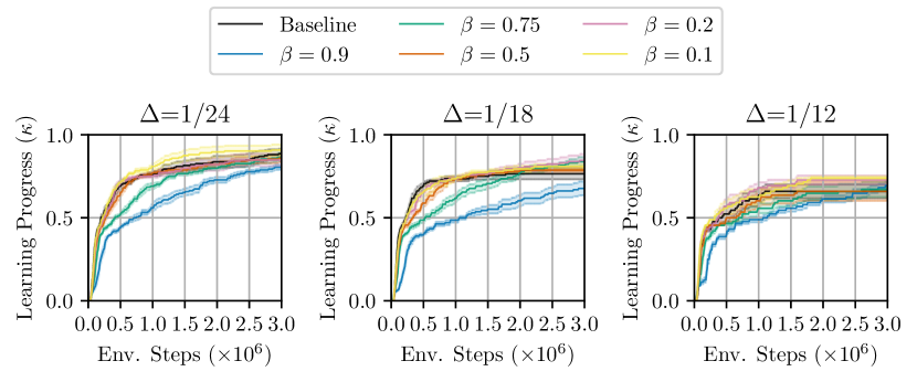
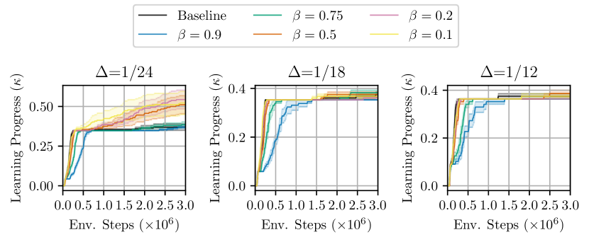
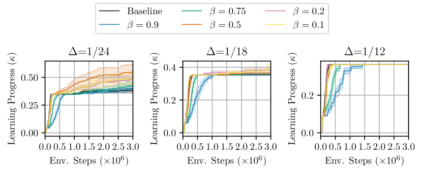
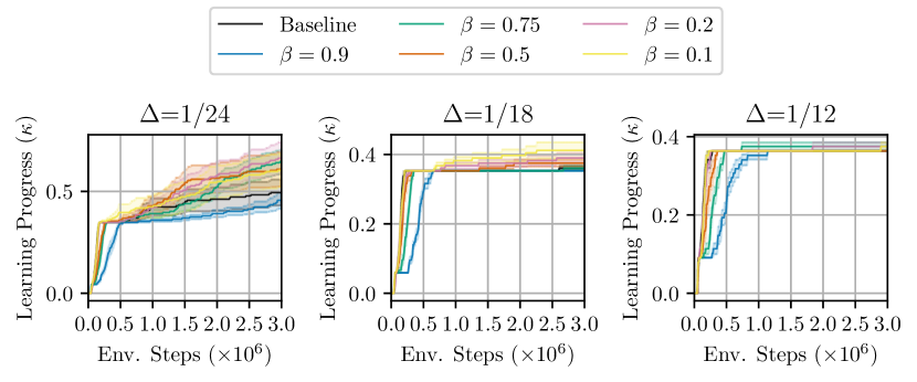
We combine Rollin with a variety of prior methods, and we evaluate the following conditions: (1) standard goal reaching; (2) goal reaching with goal relabeling (Andrychowicz et al., 2017); (3) goal reaching with an exploration phase that is similar to Go-Explore (Ecoffet et al., 2019). For goal relabeling, we adopt a similar relabeling technique as Pitis et al. (2020), where each mini-batch contains 1/3131/3 original transitions, 1/3131/3 transitions with future state relabeling, and 1/3131/3 transitions with next state relabeling. We implemented the Go-Explore method by adding an additional standard Gaussian exploration noise in the action to the agent for learning the next goal ω(k+1)𝜔𝑘1\omega(k+1), once it reaches the current goal ω(k)𝜔𝑘\omega(k). We empirically observed that sampling the replay buffer from a geometric distribution with p=105𝑝superscript105p=10^{-5} (more recent transitions are sampled more frequently) improves the overall performance. Hence, in all future experiments, we compare the performance of Rollin with classic uniform sampling and the new geometric sampling. We compare the learning speed of Rollin with parameter β=0.1𝛽0.1\beta=0.1 on three different step sizes Δ=124,118,112Δ124118112\Delta=\frac{1}{24},\frac{1}{18},\frac{1}{12} in Table 2.

Main comparisons. We first provide an overview experiments that compares Rollin with a fixed β=0.1𝛽0.1\beta=0.1 on different step sizes ΔΔ\Delta in different settings. In each case, we compare the prior method (vanilla, relabeled, or Go-Explore) with and without the addition of Rollin. As shown in Table 2, Rollin improves the largest value of κ𝜅\kappa reached by the agent in most presented settings (except Go-Explore with Δ=1/12Δ112\Delta=1/12). This result suggests that Rollin facilitates goal-conditioned RL with a curriculum, as we only update the learning progress κ𝜅\kappa to κ+Δ𝜅Δ\kappa+\Delta when the return of the current policy reaches a certain threshold R𝑅R (See detailed update of κ𝜅\kappa in Algorithm 2). Note that β=0.1𝛽0.1\beta=0.1 does not always produce the best result, we will provide more results comparing different β𝛽\betas in different settings later in this section, and we leave all the learning curves and detailed tables to Section G.1. Note that we do not include the results of directly learning the last context in the antmaze-umaze environment because the agent cannot reach the goal without the aid of a curriculum, which is corroborated by (Pitis et al., 2020).

Step = 0.5×1060.5superscript1060.5\times 10^{6} Step = 1.0×1061.0superscript1061.0\times 10^{6}
Env. Method κ𝜅\kappa x𝑥x-velocity return κ𝜅\kappa x𝑥x-velocity return
walker Scratch n/a 3.07±0.26plus-or-minus3.070.263.07\pm 0.26 3373.1±170.5plus-or-minus3373.1170.53373.1\pm 170.5 n/a 3.30±0.36plus-or-minus3.300.363.30\pm 0.36 4212.3±151.4plus-or-minus4212.3151.44212.3\pm 151.4
Baseline 0.83±0.03plus-or-minus0.830.030.83\pm 0.03 3.09±0.31plus-or-minus3.090.313.09\pm 0.31 3450.1±307.4plus-or-minus3450.1307.43450.1\pm 307.4 0.92±0.03plus-or-minus0.920.030.92\pm 0.03 3.69±0.27plus-or-minus3.690.273.69\pm 0.27 4032.3±224.3plus-or-minus4032.3224.34032.3\pm 224.3
Rollin 0.79±0.04plus-or-minus0.790.040.79\pm 0.04 2.83±0.31plus-or-minus2.830.31{2.83\pm 0.31} 3350.4±184.6plus-or-minus3350.4184.6{3350.4\pm 184.6} 0.94±0.03plus-or-minus0.940.030.94\pm 0.03 3.62±0.26plus-or-minus3.620.263.62\pm 0.26 4128.8±159.6plus-or-minus4128.8159.6{4128.8\pm 159.6}
hopper Scratch n/a 2.50±0.13plus-or-minus2.500.132.50\pm 0.13 2943.6±80.3plus-or-minus2943.680.32943.6\pm 80.3 n/a 2.55±0.12plus-or-minus2.550.122.55\pm 0.12 3073.2±137.7plus-or-minus3073.2137.73073.2\pm 137.7
Baseline 0.85±0.02plus-or-minus0.850.020.85\pm 0.02 2.42±0.18plus-or-minus2.420.182.42\pm 0.18 3192.5±80.4plus-or-minus3192.580.43192.5\pm 80.4 0.88±0.01plus-or-minus0.880.010.88\pm 0.01 2.58±0.16plus-or-minus2.580.162.58\pm 0.16 3386.2±124.7plus-or-minus3386.2124.73386.2\pm 124.7
Rollin 0.82±0.03plus-or-minus0.820.030.82\pm 0.03 2.26±0.22plus-or-minus2.260.222.26\pm 0.22 3148.6±160.7plus-or-minus3148.6160.7{3148.6\pm 160.7} 0.89±0.00plus-or-minus0.890.000.89\pm 0.00 2.65±0.15plus-or-minus2.650.152.65\pm 0.15 3421.9±109.8plus-or-minus3421.9109.8{3421.9\pm 109.8}
humanoid Scratch n/a 0.24±0.05plus-or-minus0.240.050.24\pm 0.05 2417.1±188.2plus-or-minus2417.1188.22417.1\pm 188.2 n/a 0.37±0.05plus-or-minus0.370.050.37\pm 0.05 2763.8±96.5plus-or-minus2763.896.52763.8\pm 96.5
Baseline 0.32±0.05plus-or-minus0.320.050.32\pm 0.05 0.26±0.05plus-or-minus0.260.050.26\pm 0.05 2910.1±262.9plus-or-minus2910.1262.92910.1\pm 262.9 0.67±0.03plus-or-minus0.670.030.67\pm 0.03 0.39±0.05plus-or-minus0.390.050.39\pm 0.05 3017.2±169.0plus-or-minus3017.2169.03017.2\pm 169.0
Rollin 0.36±0.04plus-or-minus0.360.040.36\pm 0.04 0.32±0.07plus-or-minus0.320.070.32\pm 0.07 2939.7±392.0plus-or-minus2939.7392.02939.7\pm 392.0 0.69±0.06plus-or-minus0.690.060.69\pm 0.06 0.46±0.09plus-or-minus0.460.090.46\pm 0.09 3173.6±238.3plus-or-minus3173.6238.33173.6\pm 238.3
ant Scratch n/a 3.60±0.49plus-or-minus3.600.493.60\pm 0.49 2910.7±354.3plus-or-minus2910.7354.32910.7\pm 354.3 n/a 4.55±0.36plus-or-minus4.550.364.55\pm 0.36 4277.9±120.0plus-or-minus4277.9120.04277.9\pm 120.0
Baseline 0.72±0.02plus-or-minus0.720.020.72\pm 0.02 3.38±0.43plus-or-minus3.380.433.38\pm 0.43 2976.2±252.4plus-or-minus2976.2252.42976.2\pm 252.4 1.00±0.00plus-or-minus1.000.001.00\pm 0.00 4.29±0.51plus-or-minus4.290.514.29\pm 0.51 4248.5±88.6plus-or-minus4248.588.64248.5\pm 88.6
Rollin 0.82±0.06plus-or-minus0.820.060.82\pm 0.06 3.85±0.41plus-or-minus3.850.413.85\pm 0.41 3593.1±237.8plus-or-minus3593.1237.83593.1\pm 237.8 1.00±0.00plus-or-minus1.000.001.00\pm 0.00 4.66±0.30plus-or-minus4.660.304.66\pm 0.30 4473.0±102.2plus-or-minus4473.0102.24473.0\pm 102.2
Table 3: Learning progress κ𝜅\kappa, average x𝑥x-velocity, and average return at 0.5 and 1.0 million environment steps in walker, hopper, humanoid, and ant. The average x𝑥x-velocity and return are estimated using the last 50k environment steps. “Scratch” shows the results of directly training the agent with the last context ω(1)𝜔1\omega(1). “Baseline” indicates β=0𝛽0\beta=0, where we provide the curriculum ω(κ)𝜔𝜅\omega(\kappa) to the agent without using Rollin. We pick β=0.1𝛽0.1\beta=0.1 for all experiments using Rollin, the results of using other β𝛽\betas can be found in Table 11, Table 12, and Table 13 in Section G.2. The standard error is computed over 8 random seeds.

6.2 Non-Goal Reaching Tasks

For the non-goal tasks, we consider the tasks of gradually increasing the x𝑥x-velocity of a locomotion agent in the following environments: walker2d, hopper, humanoid, and ant in OpenAI gym (Brockman et al., 2016). More specifically, we set the desired speed range to be [λκ,λ(κ+0.1))𝜆𝜅𝜆𝜅0.1[\lambda\kappa,\lambda(\kappa+0.1)), where λ𝜆\lambda is a parameter depending on the physics of the agent in different environments and we choose a fixed contextual space with ten discrete contexts: κ{0.1,0.2,,1}𝜅0.10.21\kappa\in\{0.1,0.2,\dots,1\}. The agent receives a higher reward when the x𝑥x-velocity is within the desired speed range and a lower reward otherwise. In each environment, we increase the task difficulty with later curriculum steps (larger κ𝜅\kappa), by increasing the near-optimal threshold R(κ)𝑅𝜅R(\kappa). Detailed parameters of the desired speed range λ𝜆\lambda, near optimal-threshold R(κ)𝑅𝜅R(\kappa), and the reward functions are in Section E.2.

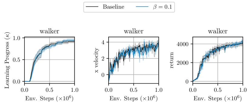
Main comparisons. We first compare Rollin with a fixed β=0.1𝛽0.1\beta=0.1 at different environment steps: 0.5×1060.5superscript1060.5\times 10^{6}, 1×1061superscript1061\times 10^{6}. In each case, we compare the learning progress κ𝜅\kappa, averaged x𝑥x-velocity, and averaged return, with and without the addition of Rollin. Note that for the case without Rollin, we still provide the curriculum to the agent for training. The results in Table 3 show that Rollin improves most benchmarks (See detailed update of κ𝜅\kappa in Algorithm 2). Note that β=0.1𝛽0.1\beta=0.1 does not always produce the best result, and we provide more results comparing different β𝛽\betas in different settings later in this section, with learning curves and more detailed tables in Section G.2.

6.3 Experimental Summary

We empirically showed that Rollin improves the performance of one goal-reaching task and four non-goal tasks in different settings. Although Rollin introduces an extra parameter β𝛽\beta, our experiments show reasonable improvement by simply choosing β=0.1𝛽0.1\beta=0.1 or 0.20.20.2. More careful selection of β𝛽\beta might lead to further improvements.

7 Discussion and Future Work

We presented Rollin, a simple algorithm that accelerates curriculum learning under the contextual MDP setup by rolling in a near-optimal policy to bootstrap the learning of new nearby contexts with provable learning efficiency benefits. Theoretically, we show that Rollin attains polynomial sample complexity by utilizing adjacent contexts to initialize each policy. Since the key theoretical insight of Rollin suggests that one can reduce the density mismatch ratio by constructing a new initial distribution, it would be interesting to see how Rollin can affect other variants of convergence analysis of PG (e.g., NPG (Kakade, 2001; Cen et al., 2021) or PG in a feature space (Agarwal et al., 2021, 2020)). On the empirical side, our experiments demonstrate that Rollin improves the empirical performance of various tasks beyond our theoretical assumptions, which reveals the potential of Rollin in other practical RL tasks with a curriculum. Our initial practical instantiation of the Rollin algorithm has a lot of room for future research. First of all, our implementation requires domain-specific knowledge of a “good” return value as it currently rely on a fixed return threshold R𝑅R to determine when we are going to switch from the current context to the next context. Another promising direction is to combine our algorithm with context-based meta-RL methods such as learning to generate sub-goal/context to accelerate the learning of the current sub-goal/context. Finally, our method is not specific to the goal-conditioned settings, which opens up the possibility of applying our algorithm to more challenging domains.

8 Acknowledgements

We are thankful to Laura Smith, Dibya Ghosh, Chuer Pan, and other members of the RAIL lab for feedback and suggestions on earlier drafts. QL would like acknowledge the support of the Berkeley Fellowship. YZ would like to thank Jincheng Mei from Google and Yuhao Ding from UC Berkeley for insightful discussions on the related proof. YM would like to acknowledge the support of ONR grants N00014-20-1-2002, N00014-22-1-2102, the joint Simons Foundation-NSF DMS grant # 2031899, and Tsinghua-Berkeley Shenzhen Institute (TBSI) Research Fund. SL would like to acknowledge Air Force Office of Scientific Research AFOSR FA9550-22-1-0273. The research is supported by Savio computational cluster provided by the Berkeley Research Compute program.

References

  • Abbasi-Yadkori and Neu (2014) Yasin Abbasi-Yadkori and Gergely Neu. Online learning in MDPs with side information. arXiv preprint arXiv:1406.6812, 2014.
  • Agarwal et al. (2019) Alekh Agarwal, Nan Jiang, Sham M Kakade, and Wen Sun. Reinforcement learning: Theory and algorithms. CS Dept., UW Seattle, Seattle, WA, USA, Tech. Rep, 2019.
  • Agarwal et al. (2020) Alekh Agarwal, Mikael Henaff, Sham Kakade, and Wen Sun. PC-PG: Policy cover directed exploration for provable policy gradient learning. Advances in Neural Information Processing Systems, 33:13399–13412, 2020.
  • Agarwal et al. (2021) Alekh Agarwal, Sham M Kakade, Jason D Lee, and Gaurav Mahajan. On the theory of policy gradient methods: Optimality, approximation, and distribution shift. Journal of Machine Learning Research, 22(98):1–76, 2021.
  • Agarwal et al. (2022) Alekh Agarwal, Yuda Song, Wen Sun, Kaiwen Wang, Mengdi Wang, and Xuezhou Zhang. Provable benefits of representational transfer in reinforcement learning. arXiv preprint arXiv:2205.14571, 2022.
  • Akkaya et al. (2019) Ilge Akkaya, Marcin Andrychowicz, Maciek Chociej, Mateusz Litwin, Bob McGrew, Arthur Petron, Alex Paino, Matthias Plappert, Glenn Powell, Raphael Ribas, et al. Solving rubik’s cube with a robot hand. arXiv preprint arXiv:1910.07113, 2019.
  • Andreas et al. (2017) Jacob Andreas, Dan Klein, and Sergey Levine. Modular multitask reinforcement learning with policy sketches. In International Conference on Machine Learning, pages 166–175. PMLR, 2017.
  • Andrychowicz et al. (2017) Marcin Andrychowicz, Filip Wolski, Alex Ray, Jonas Schneider, Rachel Fong, Peter Welinder, Bob McGrew, Josh Tobin, OpenAI Pieter Abbeel, and Wojciech Zaremba. Hindsight experience replay. Advances in neural information processing systems, 30, 2017.
  • Andrychowicz et al. (2020) OpenAI: Marcin Andrychowicz, Bowen Baker, Maciek Chociej, Rafal Jozefowicz, Bob McGrew, Jakub Pachocki, Arthur Petron, Matthias Plappert, Glenn Powell, Alex Ray, et al. Learning dexterous in-hand manipulation. The International Journal of Robotics Research, 39(1):3–20, 2020.
  • Åström and Wittenmark (2013) Karl J Åström and Björn Wittenmark. Adaptive control. Courier Corporation, 2013.
  • Azar et al. (2017) Mohammad Gheshlaghi Azar, Ian Osband, and Rémi Munos. Minimax regret bounds for reinforcement learning. In International Conference on Machine Learning, pages 263–272. PMLR, 2017.
  • Bassich et al. (2020) Andrea Bassich, Francesco Foglino, Matteo Leonetti, and Daniel Kudenko. Curriculum learning with a progression function. arXiv preprint arXiv:2008.00511, 2020.
  • Bellemare et al. (2016) Marc Bellemare, Sriram Srinivasan, Georg Ostrovski, Tom Schaul, David Saxton, and Remi Munos. Unifying count-based exploration and intrinsic motivation. In Advances in Neural Information Processing Systems, pages 1471–1479, 2016.
  • Belogolovsky et al. (2021) Stav Belogolovsky, Philip Korsunsky, Shie Mannor, Chen Tessler, and Tom Zahavy. Inverse reinforcement learning in contextual MDPs. Machine Learning, 110(9):2295–2334, 2021.
  • Berner et al. (2019) Christopher Berner, Greg Brockman, Brooke Chan, Vicki Cheung, Przemysław Dębiak, Christy Dennison, David Farhi, Quirin Fischer, Shariq Hashme, Chris Hesse, et al. Dota 2 with large scale deep reinforcement learning. arXiv preprint arXiv:1912.06680, 2019.
  • Bhandari and Russo (2019) Jalaj Bhandari and Daniel Russo. Global optimality guarantees for policy gradient methods. arXiv preprint arXiv:1906.01786, 2019.
  • Brockman et al. (2016) Greg Brockman, Vicki Cheung, Ludwig Pettersson, Jonas Schneider, John Schulman, Jie Tang, and Wojciech Zaremba. OpenAI Gym, 2016.
  • Burda et al. (2018) Yuri Burda, Harrison Edwards, Amos Storkey, and Oleg Klimov. Exploration by random network distillation. arXiv preprint arXiv:1810.12894, 2018.
  • Cen et al. (2021) Shicong Cen, Chen Cheng, Yuxin Chen, Yuting Wei, and Yuejie Chi. Fast global convergence of natural policy gradient methods with entropy regularization. Operations Research, 2021.
  • Dann et al. (2019) Christoph Dann, Lihong Li, Wei Wei, and Emma Brunskill. Policy certificates: Towards accountable reinforcement learning. In International Conference on Machine Learning, pages 1507–1516. PMLR, 2019.
  • Dennis et al. (2020) Michael Dennis, Natasha Jaques, Eugene Vinitsky, Alexandre Bayen, Stuart Russell, Andrew Critch, and Sergey Levine. Emergent complexity and zero-shot transfer via unsupervised environment design. Advances in Neural Information Processing Systems, 33:13049–13061, 2020.
  • D’Eramo et al. (2020) Carlo D’Eramo, Davide Tateo, Andrea Bonarini, Marcello Restelli, and Jan Peters. Sharing knowledge in multi-task deep reinforcement learning. In International Conference on Learning Representations, 2020. URL https://openreview.net/forum?id=rkgpv2VFvr.
  • Ding et al. (2021) Yuhao Ding, Junzi Zhang, and Javad Lavaei. Beyond exact gradients: Convergence of stochastic soft-max policy gradient methods with entropy regularization. arXiv preprint arXiv:2110.10117, 2021.
  • Du et al. (2019) Simon Du, Akshay Krishnamurthy, Nan Jiang, Alekh Agarwal, Miroslav Dudik, and John Langford. Provably efficient RL with rich observations via latent state decoding. In International Conference on Machine Learning, pages 1665–1674. PMLR, 2019.
  • Ecoffet et al. (2019) Adrien Ecoffet, Joost Huizinga, Joel Lehman, Kenneth O Stanley, and Jeff Clune. Go-Explore: a new approach for hard-exploration problems. arXiv preprint arXiv:1901.10995, 2019.
  • Eysenbach et al. (2020a) Ben Eysenbach, Xinyang Geng, Sergey Levine, and Russ R Salakhutdinov. Rewriting history with inverse rl: Hindsight inference for policy improvement. Advances in neural information processing systems, 33:14783–14795, 2020a.
  • Eysenbach et al. (2020b) Benjamin Eysenbach, Ruslan Salakhutdinov, and Sergey Levine. C-learning: Learning to achieve goals via recursive classification. arXiv preprint arXiv:2011.08909, 2020b.
  • Fang et al. (2020) Kuan Fang, Yuke Zhu, Silvio Savarese, and Li Fei-Fei. Adaptive procedural task generation for hard-exploration problems. arXiv preprint arXiv:2007.00350, 2020.
  • Fazel et al. (2018) Maryam Fazel, Rong Ge, Sham Kakade, and Mehran Mesbahi. Global convergence of policy gradient methods for the linear quadratic regulator. In International Conference on Machine Learning, pages 1467–1476. PMLR, 2018.
  • Finn et al. (2017) Chelsea Finn, Pieter Abbeel, and Sergey Levine. Model-agnostic meta-learning for fast adaptation of deep networks. In International conference on machine learning, pages 1126–1135. PMLR, 2017.
  • Florensa et al. (2017) Carlos Florensa, David Held, Markus Wulfmeier, Michael Zhang, and Pieter Abbeel. Reverse curriculum generation for reinforcement learning. In Conference on robot learning, pages 482–495. PMLR, 2017.
  • Florensa et al. (2018) Carlos Florensa, David Held, Xinyang Geng, and Pieter Abbeel. Automatic goal generation for reinforcement learning agents. In International conference on machine learning, pages 1515–1528. PMLR, 2018.
  • Fu et al. (2018) Justin Fu, Avi Singh, Dibya Ghosh, Larry Yang, and Sergey Levine. Variational inverse control with events: A general framework for data-driven reward definition. arXiv preprint arXiv:1805.11686, 2018.
  • Fu et al. (2020) Justin Fu, Aviral Kumar, Ofir Nachum, George Tucker, and Sergey Levine. D4RL: Datasets for deep data-driven reinforcement learning. arXiv preprint arXiv:2004.07219, 2020.
  • Fujita et al. (2020) Yasuhiro Fujita, Kota Uenishi, Avinash Ummadisingu, Prabhat Nagarajan, Shimpei Masuda, and Mario Ynocente Castro. Distributed reinforcement learning of targeted grasping with active vision for mobile manipulators. In 2020 IEEE/RSJ International Conference on Intelligent Robots and Systems (IROS), pages 9712–9719. IEEE, 2020.
  • Ghosh et al. (2021) Dibya Ghosh, Abhishek Gupta, Ashwin Reddy, Justin Fu, Coline Manon Devin, Benjamin Eysenbach, and Sergey Levine. Learning to reach goals via iterated supervised learning. In International Conference on Learning Representations, 2021. URL https://openreview.net/forum?id=rALA0Xo6yNJ.
  • Goodwin and Sin (2014) Graham C Goodwin and Kwai Sang Sin. Adaptive filtering prediction and control. Courier Corporation, 2014.
  • Goyal et al. (2019) Anirudh Goyal, Riashat Islam, DJ Strouse, Zafarali Ahmed, Hugo Larochelle, Matthew Botvinick, Sergey Levine, and Yoshua Bengio. Transfer and exploration via the information bottleneck. In International Conference on Learning Representations, 2019. URL https://openreview.net/forum?id=rJg8yhAqKm.
  • Goyal et al. (2020) Anirudh Goyal, Yoshua Bengio, Matthew Botvinick, and Sergey Levine. The variational bandwidth bottleneck: Stochastic evaluation on an information budget. In International Conference on Learning Representations, 2020. URL https://openreview.net/forum?id=Hye1kTVFDS.
  • Gupta et al. (2022) Abhishek Gupta, Aldo Pacchiano, Yuexiang Zhai, Sham M Kakade, and Sergey Levine. Unpacking reward shaping: Understanding the benefits of reward engineering on sample complexity. arXiv preprint arXiv:2210.09579, 2022.
  • Haarnoja (2018) Tuomas Haarnoja. Acquiring diverse robot skills via maximum entropy deep reinforcement learning. University of California, Berkeley, 2018.
  • Haarnoja et al. (2018) Tuomas Haarnoja, Aurick Zhou, Kristian Hartikainen, George Tucker, Sehoon Ha, Jie Tan, Vikash Kumar, Henry Zhu, Abhishek Gupta, Pieter Abbeel, et al. Soft actor-critic algorithms and applications. arXiv preprint arXiv:1812.05905, 2018.
  • Hallak et al. (2015) Assaf Hallak, Dotan Di Castro, and Shie Mannor. Contextual markov decision processes. arXiv preprint arXiv:1502.02259, 2015.
  • Hartikainen et al. (2019) Kristian Hartikainen, Xinyang Geng, Tuomas Haarnoja, and Sergey Levine. Dynamical distance learning for semi-supervised and unsupervised skill discovery. arXiv preprint arXiv:1907.08225, 2019.
  • Ivanovic et al. (2019) Boris Ivanovic, James Harrison, Apoorva Sharma, Mo Chen, and Marco Pavone. BARC: Backward reachability curriculum for robotic reinforcement learning. In 2019 International Conference on Robotics and Automation (ICRA), pages 15–21. IEEE, 2019.
  • Jiang et al. (2017) Nan Jiang, Akshay Krishnamurthy, Alekh Agarwal, John Langford, and Robert E Schapire. Contextual decision processes with low Bellman rank are PAC-learnable. In International Conference on Machine Learning, pages 1704–1713. PMLR, 2017.
  • Jin et al. (2018) Chi Jin, Zeyuan Allen-Zhu, Sebastien Bubeck, and Michael I Jordan. Is Q-learning provably efficient? Advances in neural information processing systems, 31, 2018.
  • Kakade and Langford (2002) Sham Kakade and John Langford. Approximately optimal approximate reinforcement learning. In In Proc. 19th International Conference on Machine Learning. Citeseer, 2002.
  • Kakade (2001) Sham M Kakade. A natural policy gradient. Advances in neural information processing systems, 14, 2001.
  • Kalashnikov et al. (2021) Dmitry Kalashnikov, Jacob Varley, Yevgen Chebotar, Benjamin Swanson, Rico Jonschkowski, Chelsea Finn, Sergey Levine, and Karol Hausman. MT-opt: Continuous multi-task robotic reinforcement learning at scale. arXiv preprint arXiv:2104.08212, 2021.
  • Kim and Choi (2018) Tae-Hoon Kim and Jonghyun Choi. Screenernet: Learning self-paced curriculum for deep neural networks. arXiv preprint arXiv:1801.00904, 2018.
  • Kingma and Ba (2015) Diederik P. Kingma and Jimmy Ba. Adam: A method for stochastic optimization. In International Conference on Learning Representations, 2015.
  • Klink et al. (2020) Pascal Klink, Carlo D’Eramo, Jan R Peters, and Joni Pajarinen. Self-paced deep reinforcement learning. Advances in Neural Information Processing Systems, 33:9216–9227, 2020.
  • Klink et al. (2022) Pascal Klink, Carlo D’Eramo, Jan Peters, and Joni Pajarinen. Boosted curriculum reinforcement learning. In International Conference on Learning Representations, 2022. URL https://openreview.net/forum?id=anbBFlX1tJ1.
  • Konda and Tsitsiklis (1999) Vijay Konda and John Tsitsiklis. Actor-critic algorithms. Advances in neural information processing systems, 12, 1999.
  • Kostrikov (2021) Ilya Kostrikov. JAXRL: Implementations of Reinforcement Learning algorithms in JAX, 10 2021. URL https://github.com/ikostrikov/jaxrl.
  • Kulkarni et al. (2016) Tejas D Kulkarni, Ardavan Saeedi, Simanta Gautam, and Samuel J Gershman. Deep successor reinforcement learning. arXiv preprint arXiv:1606.02396, 2016.
  • Landau et al. (2011) Ioan Doré Landau, Rogelio Lozano, Mohammed M’Saad, and Alireza Karimi. Adaptive control: algorithms, analysis and applications. Springer Science & Business Media, 2011.
  • Li et al. (2021) Gen Li, Yuting Wei, Yuejie Chi, Yuantao Gu, and Yuxin Chen. Softmax policy gradient methods can take exponential time to converge. In Conference on Learning Theory, pages 3107–3110. PMLR, 2021.
  • Liu et al. (2022) Xingyu Liu, Deepak Pathak, and Kris M Kitani. Revolver: Continuous evolutionary models for robot-to-robot policy transfer. arXiv preprint arXiv:2202.05244, 2022.
  • Mei et al. (2020) Jincheng Mei, Chenjun Xiao, Csaba Szepesvari, and Dale Schuurmans. On the global convergence rates of softmax policy gradient methods. In International Conference on Machine Learning, pages 6820–6829. PMLR, 2020.
  • Mendonca et al. (2021) Russell Mendonca, Oleh Rybkin, Kostas Daniilidis, Danijar Hafner, and Deepak Pathak. Discovering and achieving goals via world models. Advances in Neural Information Processing Systems, 34, 2021.
  • Misra et al. (2020) Dipendra Misra, Mikael Henaff, Akshay Krishnamurthy, and John Langford. Kinematic state abstraction and provably efficient rich-observation reinforcement learning. In International conference on machine learning, pages 6961–6971. PMLR, 2020.
  • Modi et al. (2018) Aditya Modi, Nan Jiang, Satinder Singh, and Ambuj Tewari. Markov decision processes with continuous side information. In Algorithmic Learning Theory, pages 597–618. PMLR, 2018.
  • Modi et al. (2020) Aditya Modi, Nan Jiang, Ambuj Tewari, and Satinder Singh. Sample complexity of reinforcement learning using linearly combined model ensembles. In International Conference on Artificial Intelligence and Statistics, pages 2010–2020. PMLR, 2020.
  • Moskovitz et al. (2022) Ted Moskovitz, Michael Arbel, Jack Parker-Holder, and Aldo Pacchiano. Towards an understanding of default policies in multitask policy optimization. In International Conference on Artificial Intelligence and Statistics, pages 10661–10686. PMLR, 2022.
  • Nachum et al. (2017) Ofir Nachum, Mohammad Norouzi, Kelvin Xu, and Dale Schuurmans. Bridging the gap between value and policy based reinforcement learning. Advances in neural information processing systems, 30, 2017.
  • Nair et al. (2020) Ashvin Nair, Shikhar Bahl, Alexander Khazatsky, Vitchyr Pong, Glen Berseth, and Sergey Levine. Contextual imagined goals for self-supervised robotic learning. In Conference on Robot Learning, pages 530–539. PMLR, 2020.
  • Nair et al. (2018) Ashvin V Nair, Vitchyr Pong, Murtaza Dalal, Shikhar Bahl, Steven Lin, and Sergey Levine. Visual reinforcement learning with imagined goals. Advances in neural information processing systems, 31, 2018.
  • Nair et al. (2022) Suraj Nair, Eric Mitchell, Kevin Chen, Silvio Savarese, Chelsea Finn, et al. Learning language-conditioned robot behavior from offline data and crowd-sourced annotation. In Conference on Robot Learning, pages 1303–1315. PMLR, 2022.
  • Narvekar et al. (2020) Sanmit Narvekar, Bei Peng, Matteo Leonetti, Jivko Sinapov, Matthew E Taylor, and Peter Stone. Curriculum learning for reinforcement learning domains: A framework and survey. arXiv preprint arXiv:2003.04960, 2020.
  • Ng et al. (1999) Andrew Y Ng, Daishi Harada, and Stuart Russell. Policy invariance under reward transformations: Theory and application to reward shaping. In ICML, volume 99, pages 278–287, 1999.
  • Omidshafiei et al. (2019) Shayegan Omidshafiei, Dong-Ki Kim, Miao Liu, Gerald Tesauro, Matthew Riemer, Christopher Amato, Murray Campbell, and Jonathan P How. Learning to teach in cooperative multiagent reinforcement learning. In Proceedings of the AAAI conference on artificial intelligence, volume 33 issue 01, pages 6128–6136, 2019.
  • OpenAI (2018) OpenAI. OpenAI Five. https://blog.openai.com/openai-five/, 2018.
  • OpenAI et al. (2021) OpenAI OpenAI, Matthias Plappert, Raul Sampedro, Tao Xu, Ilge Akkaya, Vineet Kosaraju, Peter Welinder, Ruben D’Sa, Arthur Petron, Henrique P d O Pinto, et al. Asymmetric self-play for automatic goal discovery in robotic manipulation. arXiv preprint arXiv:2101.04882, 2021.
  • Parker-Holder et al. (2022) Jack Parker-Holder, Minqi Jiang, Michael Dennis, Mikayel Samvelyan, Jakob Foerster, Edward Grefenstette, and Tim Rocktäschel. Evolving curricula with regret-based environment design. arXiv preprint arXiv:2203.01302, 2022.
  • Peters and Schaal (2008) Jan Peters and Stefan Schaal. Natural actor-critic. Neurocomputing, 71(7-9):1180–1190, 2008.
  • Pitis et al. (2020) Silviu Pitis, Harris Chan, Stephen Zhao, Bradly Stadie, and Jimmy Ba. Maximum entropy gain exploration for long horizon multi-goal reinforcement learning. In International Conference on Machine Learning, pages 7750–7761. PMLR, 2020.
  • Pong et al. (2019) Vitchyr H Pong, Murtaza Dalal, Steven Lin, Ashvin Nair, Shikhar Bahl, and Sergey Levine. Skew-fit: State-covering self-supervised reinforcement learning. arXiv preprint arXiv:1903.03698, 2019.
  • Portelas et al. (2020) Rémy Portelas, Cédric Colas, Katja Hofmann, and Pierre-Yves Oudeyer. Teacher algorithms for curriculum learning of deep rl in continuously parameterized environments. In Conference on Robot Learning, pages 835–853. PMLR, 2020.
  • Rajeswaran et al. (2016) Aravind Rajeswaran, Sarvjeet Ghotra, Balaraman Ravindran, and Sergey Levine. Epopt: Learning robust neural network policies using model ensembles. arXiv preprint arXiv:1610.01283, 2016.
  • Ren et al. (2019) Zhizhou Ren, Kefan Dong, Yuan Zhou, Qiang Liu, and Jian Peng. Exploration via hindsight goal generation. Advances in Neural Information Processing Systems, 32, 2019.
  • Rusu et al. (2015) Andrei A Rusu, Sergio Gomez Colmenarejo, Caglar Gulcehre, Guillaume Desjardins, James Kirkpatrick, Razvan Pascanu, Volodymyr Mnih, Koray Kavukcuoglu, and Raia Hadsell. Policy distillation. arXiv preprint arXiv:1511.06295, 2015.
  • Sastry et al. (1990) Shankar Sastry, Marc Bodson, and James F Bartram. Adaptive control: stability, convergence, and robustness, 1990.
  • Schulman et al. (2015) John Schulman, Sergey Levine, Pieter Abbeel, Michael Jordan, and Philipp Moritz. Trust region policy optimization. In International conference on machine learning, pages 1889–1897. PMLR, 2015.
  • Schulman et al. (2017) John Schulman, Filip Wolski, Prafulla Dhariwal, Alec Radford, and Oleg Klimov. Proximal policy optimization algorithms. arXiv preprint arXiv:1707.06347, 2017.
  • Siriwardhana et al. (2019) Shamane Siriwardhana, Rivindu Weerasakera, Denys JC Matthies, and Suranga Nanayakkara. VUSFA: Variational universal successor features approximator to improve transfer DRL for target driven visual navigation. arXiv preprint arXiv:1908.06376, 2019.
  • Stadie et al. (2015) Bradly C Stadie, Sergey Levine, and Pieter Abbeel. Incentivizing exploration in reinforcement learning with deep predictive models. arXiv preprint arXiv:1507.00814, 2015.
  • Sukhbaatar et al. (2018) Sainbayar Sukhbaatar, Emily Denton, Arthur Szlam, and Rob Fergus. Learning goal embeddings via self-play for hierarchical reinforcement learning. arXiv preprint arXiv:1811.09083, 2018.
  • Sun et al. (2019) Wen Sun, Nan Jiang, Akshay Krishnamurthy, Alekh Agarwal, and John Langford. Model-based RL in contextual decision processes: PAC bounds and exponential improvements over model-free approaches. In Conference on learning theory, pages 2898–2933. PMLR, 2019.
  • Sutton et al. (1999) Richard S Sutton, David McAllester, Satinder Singh, and Yishay Mansour. Policy gradient methods for reinforcement learning with function approximation. Advances in neural information processing systems, 12, 1999.
  • Tanaka and Yamamura (2003) Fumihide Tanaka and Masayuki Yamamura. Multitask reinforcement learning on the distribution of MDPs. In Proceedings 2003 IEEE International Symposium on Computational Intelligence in Robotics and Automation. Computational Intelligence in Robotics and Automation for the New Millennium (Cat. No. 03EX694), volume 3, pages 1108–1113. IEEE, 2003.
  • Tang et al. (2017) Haoran Tang, Rein Houthooft, Davis Foote, Adam Stooke, OpenAI Xi Chen, Yan Duan, John Schulman, Filip DeTurck, and Pieter Abbeel. # exploration: A study of count-based exploration for deep reinforcement learning. In Advances in neural information processing systems, pages 2753–2762, 2017.
  • Tao (2003) Gang Tao. Adaptive control design and analysis, volume 37. John Wiley & Sons, 2003.
  • Vinyals et al. (2019) Oriol Vinyals, Igor Babuschkin, Wojciech M Czarnecki, Michaël Mathieu, Andrew Dudzik, Junyoung Chung, David H Choi, Richard Powell, Timo Ewalds, Petko Georgiev, et al. Grandmaster level in starcraft ii using multi-agent reinforcement learning. Nature, 575(7782):350–354, 2019.
  • Warde-Farley et al. (2018) David Warde-Farley, Tom Van de Wiele, Tejas Kulkarni, Catalin Ionescu, Steven Hansen, and Volodymyr Mnih. Unsupervised control through non-parametric discriminative rewards. arXiv preprint arXiv:1811.11359, 2018.
  • Williams (1992) Ronald J Williams. Simple statistical gradient-following algorithms for connectionist reinforcement learning. Machine learning, 8(3-4):229–256, 1992.
  • Ye et al. (2020) Deheng Ye, Guibin Chen, Wen Zhang, Sheng Chen, Bo Yuan, Bo Liu, Jia Chen, Zhao Liu, Fuhao Qiu, Hongsheng Yu, Yinyuting Yin, Bei Shi, Liang Wang, Tengfei Shi, Qiang Fu, Wei Yang, Lanxiao Huang, and Wei Liu. Towards playing full moba games with deep reinforcement learning. In H. Larochelle, M. Ranzato, R. Hadsell, M. F. Balcan, and H. Lin, editors, Advances in Neural Information Processing Systems, volume 33, pages 621–632. Curran Associates, Inc., 2020. URL https://proceedings.neurips.cc/paper/2020/file/06d5ae105ea1bea4d800bc96491876e9-Paper.pdf.
  • Yu et al. (2020a) Tianhe Yu, Saurabh Kumar, Abhishek Gupta, Sergey Levine, Karol Hausman, and Chelsea Finn. Gradient surgery for multi-task learning. Advances in Neural Information Processing Systems, 33:5824–5836, 2020a.
  • Yu et al. (2020b) Tianhe Yu, Deirdre Quillen, Zhanpeng He, Ryan Julian, Karol Hausman, Chelsea Finn, and Sergey Levine. Meta-world: A benchmark and evaluation for multi-task and meta reinforcement learning. In Conference on Robot Learning, pages 1094–1100. PMLR, 2020b.
  • Yuan et al. (2022) Rui Yuan, Robert M Gower, and Alessandro Lazaric. A general sample complexity analysis of vanilla policy gradient. In International Conference on Artificial Intelligence and Statistics, pages 3332–3380. PMLR, 2022.
  • Zhai et al. (2022) Yuexiang Zhai, Christina Baek, Zhengyuan Zhou, Jiantao Jiao, and Yi Ma. Computational benefits of intermediate rewards for goal-reaching policy learning. Journal of Artificial Intelligence Research, 73:847–896, 2022.
  • Zhang et al. (2020a) Junzi Zhang, Jongho Kim, Brendan O’Donoghue, and Stephen Boyd. Sample efficient reinforcement learning with reinforce. arXiv preprint arXiv:2010.11364, page 97, 2020a.
  • Zhang et al. (2020b) Kaiqing Zhang, Alec Koppel, Hao Zhu, and Tamer Basar. Global convergence of policy gradient methods to (almost) locally optimal policies. SIAM Journal on Control and Optimization, 58(6):3586–3612, 2020b.
  • Zhang et al. (2021) Tianjun Zhang, Benjamin Eysenbach, Ruslan Salakhutdinov, Sergey Levine, and Joseph E Gonzalez. C-planning: An automatic curriculum for learning goal-reaching tasks. arXiv preprint arXiv:2110.12080, 2021.
  • Zhang et al. (2020c) Yunzhi Zhang, Pieter Abbeel, and Lerrel Pinto. Automatic curriculum learning through value disagreement. Advances in Neural Information Processing Systems, 33:7648–7659, 2020c.
  • Zhang et al. (2020d) Zihan Zhang, Yuan Zhou, and Xiangyang Ji. Almost optimal model-free reinforcement learningvia reference-advantage decomposition. Advances in Neural Information Processing Systems, 33:15198–15207, 2020d.

Appendix A Generalization Between Different Tasks in the Context Space

A.1 Summaries of Notations and Assumptions

  1. 1.

    The maximum entropy RL (MaxEnt RL) objective with initial state distribution ρ𝜌\rho in reinforcement aims at maximizing (Equation 15 & 16 of [Mei et al., 2020])

    Vπ(ρ):=h=0γh𝔼s0ρ,ahπ(ah|sh)[r(sh,ah)]+α(ρ,π)assignsuperscript𝑉𝜋𝜌superscriptsubscript0superscript𝛾subscript𝔼formulae-sequencesimilar-tosubscript𝑠0𝜌similar-tosubscript𝑎𝜋conditionalsubscript𝑎subscript𝑠delimited-[]𝑟subscript𝑠subscript𝑎𝛼𝜌𝜋\displaystyle V^{\pi}(\rho):=\sum_{h=0}^{\infty}\gamma^{h}\mathbb{E}_{s_{0}\sim\rho,a_{h}\sim\pi(a_{h}|s_{h})}\left[r(s_{h},a_{h})\right]+\alpha\mathbb{H}(\rho,\pi) (4)

    and (π(ah|sh))𝜋conditionalsubscript𝑎subscript𝑠\mathbb{H}(\pi(a_{h}|s_{h})) is the discounted entropy term

    (ρ,π):=𝔼s0ρ,ahπ(|sh)[h=0γhlogπ(ah|sh)],\mathbb{H}(\rho,\pi):=\underset{s_{0}\sim\rho,a_{h}\sim\pi(\cdot|s_{h})}{\mathbb{E}}\left[\sum_{h=0}^{\infty}-\gamma^{h}\log\pi(a_{h}|s_{h})\right], (5)

    and α𝛼\alpha is the penalty term. For simplicity, we denote the optimization objective function in (4) as α𝛼\alpha-MaxEnt RL. Similar to Equation 18 & 19 of [Mei et al., 2020], we also define the advantage and Q𝑄Q-functions and for MaxEnt RL as

    Aπ(s,a):=Qπ(s,a)αlogπ(s,a)Vπ(s),Qπ(s,a):=r(s,a)+γsP(s|s,a)Vπ(s).formulae-sequenceassignsuperscript𝐴𝜋𝑠𝑎superscript𝑄𝜋𝑠𝑎𝛼𝜋𝑠𝑎superscript𝑉𝜋𝑠assignsuperscript𝑄𝜋𝑠𝑎𝑟𝑠𝑎𝛾subscriptsuperscript𝑠𝑃conditionalsuperscript𝑠𝑠𝑎superscript𝑉𝜋𝑠\begin{split}A^{\pi}(s,a)&:=Q^{\pi}(s,a)-\alpha\log\pi(s,a)-V^{\pi}(s),\\ Q^{\pi}(s,a)&:=r(s,a)+\gamma\sum_{s^{\prime}}P(s^{\prime}|s,a)V^{\pi}(s).\end{split} (6)
  2. 2.

    We let

    ds0π(s)=(1γ)t=0γtπ(st=s|s0),superscriptsubscript𝑑subscript𝑠0𝜋𝑠1𝛾superscriptsubscript𝑡0superscript𝛾𝑡superscript𝜋subscript𝑠𝑡conditional𝑠subscript𝑠0d_{s_{0}}^{\pi}(s)=(1-\gamma)\sum_{t=0}^{\infty}\gamma^{t}\mathbb{P}^{\pi}(s_{t}=s|s_{0}), (7)

    to denote the discounted state visitation of policy π𝜋\pi starting at state s0subscript𝑠0s_{0}, and let

    dρπ(s)=𝔼sρ[dsπ(s)]superscriptsubscript𝑑𝜌𝜋𝑠subscript𝔼similar-to𝑠𝜌delimited-[]superscriptsubscript𝑑𝑠𝜋𝑠d_{\rho}^{\pi}(s)=\mathbb{E}_{s\sim\rho}[d_{s}^{\pi}(s)] (8)

    denote the initial state visitation distribution under initial state distribution ρ𝜌\rho.

  3. 3.

    We assume the reward functions under all context are bounded within [0,1]01[0,1]:

    rω(s,a)[0,1],ωΩ,(s,a)𝒮×𝒜.formulae-sequencesubscript𝑟𝜔𝑠𝑎01formulae-sequencefor-all𝜔Ωfor-all𝑠𝑎𝒮𝒜r_{\omega}(s,a)\in[0,1],\;\forall\omega\in\Omega,\forall(s,a)\in\mathcal{S}\times\mathcal{A}. (9)
  4. 4.

    Similar to previous analysis in [Agarwal et al., 2021, Mei et al., 2020, Ding et al., 2021], we assume the initial distribution μ𝜇\mu for PG/stochastic PG satisfies ρ(s)>0,s𝒮formulae-sequence𝜌𝑠0for-all𝑠𝒮\rho(s)>0,\forall s\in\mathcal{S}.

A.2 Main Results: Mismatch Coefficient Upper Bound

Lemma A.1 (Density Mismatch Ratio via Rollin).

Assuming ρ=Unif(𝒮)𝜌Unif𝒮\rho=\mathrm{Unif}(\mathcal{S}), and μk=βdμk1πωk1+(1β)ρsubscript𝜇𝑘𝛽subscriptsuperscript𝑑superscriptsubscript𝜋subscript𝜔𝑘1subscript𝜇𝑘11𝛽𝜌\mu_{k}=\beta d^{\pi_{\omega_{k-1}}^{\star}}_{\mu_{k-1}}+(1-\beta)\rho (using (1) from Rollin), the density mismatch ratio dμkπωk/μksubscriptnormsubscriptsuperscript𝑑subscriptsuperscript𝜋subscript𝜔𝑘subscript𝜇𝑘subscript𝜇𝑘\left\|d^{\pi^{\star}_{\omega_{k}}}_{\mu_{k}}/\mu_{k}\right\|_{\infty} satisfies

dμkπωkμkO~(Lrα(1β)ΔωkS),subscriptnormsubscriptsuperscript𝑑subscriptsuperscript𝜋subscript𝜔𝑘subscript𝜇𝑘subscript𝜇𝑘~𝑂subscript𝐿𝑟𝛼1𝛽subscriptsuperscriptΔ𝑘𝜔𝑆\left\|\frac{d^{\pi^{\star}_{\omega_{k}}}_{\mu_{k}}}{\mu_{k}}\right\|_{\infty}\leq\;\widetilde{O}\left(\frac{L_{r}}{\alpha(1-\beta)}\Delta^{k}_{\omega}S\right), (10)

where Δωk=max1ikωiωi12superscriptsubscriptΔ𝜔𝑘subscript1𝑖𝑘subscriptnormsubscript𝜔𝑖subscript𝜔𝑖12\Delta_{\omega}^{k}=\max_{1\leq i\leq k}\left\|\omega_{i}-\omega_{i-1}\right\|_{2}.

Proof.

By (1) from Rollin, we have

dμkπωkμk=dμkπωkdμk1πωk1+dμk1πωk1μk(i)dμkπωkdμk1πωk11minμk+dμk1πωk1βdμk1πωk1+(1β)ρ(ii)dμkπωkdμk1πωk11minμk+1βsubscriptdelimited-∥∥superscriptsubscript𝑑subscript𝜇𝑘subscriptsuperscript𝜋subscript𝜔𝑘subscript𝜇𝑘subscriptdelimited-∥∥superscriptsubscript𝑑subscript𝜇𝑘subscriptsuperscript𝜋subscript𝜔𝑘superscriptsubscript𝑑subscript𝜇𝑘1subscriptsuperscript𝜋subscript𝜔𝑘1superscriptsubscript𝑑subscript𝜇𝑘1subscriptsuperscript𝜋subscript𝜔𝑘1subscript𝜇𝑘𝑖subscriptnormsubscriptsuperscript𝑑subscriptsuperscript𝜋subscript𝜔𝑘subscript𝜇𝑘subscriptsuperscript𝑑subscriptsuperscript𝜋subscript𝜔𝑘1subscript𝜇𝑘11subscript𝜇𝑘subscriptdelimited-∥∥superscriptsubscript𝑑subscript𝜇𝑘1subscriptsuperscript𝜋subscript𝜔𝑘1𝛽subscriptsuperscript𝑑subscriptsuperscript𝜋subscript𝜔𝑘1subscript𝜇𝑘11𝛽𝜌𝑖𝑖subscriptnormsubscriptsuperscript𝑑subscriptsuperscript𝜋subscript𝜔𝑘subscript𝜇𝑘subscriptsuperscript𝑑subscriptsuperscript𝜋subscript𝜔𝑘1subscript𝜇𝑘11subscript𝜇𝑘1𝛽\begin{split}&\left\|\frac{d_{\mu_{k}}^{\pi^{\star}_{\omega_{k}}}}{\mu_{k}}\right\|_{\infty}=\left\|\frac{d_{\mu_{k}}^{\pi^{\star}_{\omega_{k}}}-d_{\mu_{k-1}}^{\pi^{\star}_{\omega_{k-1}}}+d_{\mu_{k-1}}^{\pi^{\star}_{\omega_{k-1}}}}{\mu_{k}}\right\|_{\infty}\\ \overset{(i)}{\leq}&\frac{\left\|d^{\pi^{\star}_{\omega_{k}}}_{\mu_{k}}-d^{\pi^{\star}_{\omega_{k-1}}}_{\mu_{k-1}}\right\|_{1}}{\min\mu_{k}}+\left\|\frac{d_{\mu_{k-1}}^{\pi^{\star}_{\omega_{k-1}}}}{\beta d^{\pi^{\star}_{\omega_{k-1}}}_{\mu_{k-1}}+(1-\beta)\rho}\right\|_{\infty}\\ \overset{(ii)}{\leq}&\frac{\left\|d^{\pi^{\star}_{\omega_{k}}}_{\mu_{k}}-d^{\pi^{\star}_{\omega_{k-1}}}_{\mu_{k-1}}\right\|_{1}}{\min\mu_{k}}+\frac{1}{\beta}\end{split} (11)

where inequality (i)𝑖(i) holds because of (1), and inequality (ii)𝑖𝑖(ii) holds because ρ(s)0,s𝒮formulae-sequence𝜌𝑠0for-all𝑠𝒮\rho(s)\geq 0,\forall s\in\mathcal{S}. Now it remains to bound dμk+1πωk+1dμkπωk1subscriptnormsubscriptsuperscript𝑑subscriptsuperscript𝜋subscript𝜔𝑘1subscript𝜇𝑘1subscriptsuperscript𝑑subscriptsuperscript𝜋subscript𝜔𝑘subscript𝜇𝑘1\left\|d^{\pi^{\star}_{\omega_{k+1}}}_{\mu_{k+1}}-d^{\pi^{\star}_{\omega_{k}}}_{\mu_{k}}\right\|_{1} using the difference ωk+1ωk2subscriptnormsubscript𝜔𝑘1subscript𝜔𝑘2\left\|\omega_{k+1}-\omega_{k}\right\|_{2}. Let hk=hπωk(s|s0μk)superscriptsubscript𝑘superscriptsubscriptsubscriptsuperscript𝜋subscript𝜔𝑘similar-toconditionalsuperscript𝑠subscript𝑠0subscript𝜇𝑘\mathbb{P}_{h}^{k}=\mathbb{P}_{h}^{\pi^{\star}_{\omega_{k}}}(s^{\prime}|s_{0}\sim\mu_{k}) denote the state visitation distribution resulting from πωksuperscriptsubscript𝜋subscript𝜔𝑘\pi_{\omega_{k}}^{\star} probability starting at μksubscript𝜇𝑘\mu_{k}, then we have

hk(s)hk1(s)=s,a(h1k(s)πωk(a|s)h1k1(s)πωk1(a|s))P(s|s,a)=s,a(h1k(s)πωk(a|s)h1k(s)πωk1(a|s)+h1k1(s)πωk1(a|s)h1k1(s)πωk1(a|s))P(s|s,a)=sh1k(s)[a(πωk(a|s)πωk1(a|s))P(s|s,a)]+s(h1k(s)h1k1(s))[aπωk1(a|s)P(s|s,a)].subscriptsuperscript𝑘superscript𝑠subscriptsuperscript𝑘1superscript𝑠subscript𝑠𝑎subscriptsuperscript𝑘1𝑠superscriptsubscript𝜋subscript𝜔𝑘conditional𝑎𝑠subscriptsuperscript𝑘11𝑠subscriptsuperscript𝜋subscript𝜔𝑘1conditional𝑎𝑠𝑃conditionalsuperscript𝑠𝑠𝑎subscript𝑠𝑎subscriptsuperscript𝑘1𝑠subscriptsuperscript𝜋subscript𝜔𝑘conditional𝑎𝑠subscriptsuperscript𝑘1𝑠subscriptsuperscript𝜋subscript𝜔𝑘1conditional𝑎𝑠subscriptsuperscript𝑘11𝑠subscriptsuperscript𝜋subscript𝜔𝑘1conditional𝑎𝑠subscriptsuperscript𝑘11𝑠subscriptsuperscript𝜋subscript𝜔𝑘1conditional𝑎𝑠𝑃conditionalsuperscript𝑠𝑠𝑎subscript𝑠superscriptsubscript1𝑘𝑠delimited-[]subscript𝑎subscriptsuperscript𝜋subscript𝜔𝑘conditional𝑎𝑠subscriptsuperscript𝜋subscript𝜔𝑘1conditional𝑎𝑠𝑃conditionalsuperscript𝑠𝑠𝑎subscript𝑠superscriptsubscript1𝑘𝑠superscriptsubscript1𝑘1𝑠delimited-[]subscript𝑎subscriptsuperscript𝜋subscript𝜔𝑘1conditional𝑎𝑠𝑃conditionalsuperscript𝑠𝑠𝑎\begin{split}&\mathbb{P}^{k}_{h}(s^{\prime})-\mathbb{P}^{k-1}_{h}(s^{\prime})=\sum_{s,a}\left(\mathbb{P}^{k}_{h-1}(s)\pi_{\omega_{k}}^{\star}(a|s)-\mathbb{P}^{k-1}_{h-1}(s)\pi^{\star}_{\omega_{k-1}}(a|s)\right)P(s^{\prime}|s,a)\\ =&\sum_{s,a}\left(\mathbb{P}^{k}_{h-1}(s)\pi^{\star}_{\omega_{k}}(a|s)-\mathbb{P}^{k}_{h-1}(s)\pi^{\star}_{\omega_{k-1}}(a|s)+\mathbb{P}^{k-1}_{h-1}(s)\pi^{\star}_{\omega_{k-1}}(a|s)-\mathbb{P}^{k-1}_{h-1}(s)\pi^{\star}_{\omega_{k-1}}(a|s)\right)P(s^{\prime}|s,a)\\ =&\sum_{s}\mathbb{P}_{h-1}^{k}(s)\left[\sum_{a}\left(\pi^{\star}_{\omega_{k}}(a|s)-\pi^{\star}_{\omega_{k-1}}(a|s)\right)P(s^{\prime}|s,a)\right]\\ &+\sum_{s}\left(\mathbb{P}_{h-1}^{k}(s)-\mathbb{P}_{h-1}^{k-1}(s)\right)\left[\sum_{a}\pi^{\star}_{\omega_{k-1}}(a|s)P(s^{\prime}|s,a)\right].\end{split} (12)

Taking absolute value on both side, yields

hkhk11=s|hk(s)hk1(s)|sh1k(s)a|πωk(a|s)πωk1(a|s)|c1ωkωk12sP(s|s,a)+s|h1k(s)h1k1(s)|[saπωk1(a|s)P(s|s,a)](i)c1ωkωk12+h1kh1k11c1hωkωk12+0k0k11=(ii)c1hωkωk12+μkμk11,\begin{split}&\left\|\mathbb{P}_{h}^{k}-\mathbb{P}_{h}^{k-1}\right\|_{1}=\sum_{s^{\prime}}\left|\mathbb{P}^{k}_{h}(s^{\prime})-\mathbb{P}^{k-1}_{h}(s^{\prime})\right|\\ \overset{}{\leq}&\sum_{s}\mathbb{P}_{h-1}^{k}(s)\sum_{a}\underbrace{\left|\pi^{\star}_{\omega_{k}}(a|s)-\pi^{\star}_{\omega_{k-1}}(a|s)\right|}_{\leq c_{1}\left\|\omega_{k}-\omega_{k-1}\right\|_{2}}\sum_{s^{\prime}}P(s^{\prime}|s,a)\\ &+\sum_{s}\left|\mathbb{P}_{h-1}^{k}(s)-\mathbb{P}_{h-1}^{k-1}(s)\right|\left[\sum_{s^{\prime}}\sum_{a}\pi^{\star}_{\omega_{k-1}}(a|s)P(s^{\prime}|s,a)\right]\\ \overset{(i)}{\leq}&c_{1}\left\|\omega_{k}-\omega_{k-1}\right\|_{2}+\left\|\mathbb{P}_{h-1}^{k}-\mathbb{P}_{h-1}^{k-1}\right\|_{1}\leq\dots\leq c_{1}h\left\|\omega_{k}-\omega_{k-1}\right\|_{2}+\left\|\mathbb{P}_{0}^{k}-\mathbb{P}_{0}^{k-1}\right\|_{1}\\ \overset{(ii)}{=}&c_{1}h\left\|\omega_{k}-\omega_{k-1}\right\|_{2}+\left\|\mu_{k}-\mu_{k-1}\right\|_{1},\end{split} (13)

where inequality (i)𝑖(i) holds by applying Lemma B.2 with c1=Lr/α(1γ)subscript𝑐1subscript𝐿𝑟𝛼1𝛾c_{1}=L_{r}/\alpha(1-\gamma) and equality (ii)𝑖𝑖(ii) holds because the initial distribution of hksuperscriptsubscript𝑘\mathbb{P}_{h}^{k} is μksubscript𝜇𝑘\mu_{k}. By the definition of dμπsuperscriptsubscript𝑑𝜇𝜋d_{\mu}^{\pi}, we have

dμkπωk(s)dμk1πωk1(s)=(i)dk(s)dk1(s)=(1γ)h=0γh(hk(s)hk1(s)),s𝒮.formulae-sequencesuperscriptsubscript𝑑subscript𝜇𝑘subscriptsuperscript𝜋subscript𝜔𝑘𝑠subscriptsuperscript𝑑subscriptsuperscript𝜋subscript𝜔𝑘1subscript𝜇𝑘1𝑠𝑖subscript𝑑𝑘𝑠subscript𝑑𝑘1𝑠1𝛾superscriptsubscript0superscript𝛾superscriptsubscript𝑘𝑠superscriptsubscript𝑘1𝑠for-all𝑠𝒮d_{\mu_{k}}^{\pi^{\star}_{\omega_{k}}}(s)-d^{\pi^{\star}_{\omega_{k-1}}}_{\mu_{k-1}}(s)\overset{(i)}{=}d_{k}(s)-d_{k-1}(s)=(1-\gamma)\sum_{h=0}^{\infty}\gamma^{h}\left(\mathbb{P}_{h}^{k}(s)-\mathbb{P}_{h}^{k-1}(s)\right),\;\forall s\in\mathcal{S}. (14)

where in equality (i)𝑖(i), we use dksubscript𝑑𝑘d_{k} to denote dμkπωksuperscriptsubscript𝑑subscript𝜇𝑘subscriptsuperscript𝜋subscript𝜔𝑘d_{\mu_{k}}^{\pi^{\star}_{\omega_{k}}}. Adding 1superscript1\ell^{1} norm on both sides of (14) and applying (13), yields

dkdk11(1γ)h=0γh(c1hωkωk12+μkμk11)=(i)γc11γωkωk12+μkμk11=(ii)γc11γωkωk12+βdk1dk21,subscriptdelimited-∥∥subscript𝑑𝑘subscript𝑑𝑘111𝛾superscriptsubscript0superscript𝛾subscript𝑐1subscriptdelimited-∥∥subscript𝜔𝑘subscript𝜔𝑘12subscriptdelimited-∥∥subscript𝜇𝑘subscript𝜇𝑘11𝑖𝛾subscript𝑐11𝛾subscriptdelimited-∥∥subscript𝜔𝑘subscript𝜔𝑘12subscriptdelimited-∥∥subscript𝜇𝑘subscript𝜇𝑘11𝑖𝑖𝛾subscript𝑐11𝛾subscriptdelimited-∥∥subscript𝜔𝑘subscript𝜔𝑘12𝛽subscriptdelimited-∥∥subscript𝑑𝑘1subscript𝑑𝑘21\begin{split}&\left\|d_{k}-d_{k-1}\right\|_{1}\leq(1-\gamma)\sum_{h=0}^{\infty}\gamma^{h}\left(c_{1}h\left\|\omega_{k}-\omega_{k-1}\right\|_{2}+\left\|\mu_{k}-\mu_{k-1}\right\|_{1}\right)\\ \overset{(i)}{=}&\frac{\gamma c_{1}}{1-\gamma}\left\|\omega_{k}-\omega_{k-1}\right\|_{2}+\left\|\mu_{k}-\mu_{k-1}\right\|_{1}\overset{(ii)}{=}\frac{\gamma c_{1}}{1-\gamma}\left\|\omega_{k}-\omega_{k-1}\right\|_{2}+\beta\left\|d_{k-1}-d_{k-2}\right\|_{1},\end{split} (15)

where equality (i)𝑖(i) holds because h=0γhh=γ/(1γ)2superscriptsubscript0superscript𝛾𝛾superscript1𝛾2\sum_{h=0}^{\infty}\gamma^{h}h=\gamma/(1-\gamma)^{2} and equality (ii)𝑖𝑖(ii) holds because of (1). Hence, we know that

dkdk11γc11γωkωk12+βdk1dk21γc11γi=0k1[ωi+1ωi2βki]+βk1d1d01γc11γ11βΔωk+βk1d1d01(γc1(1γ)(1β)+1)Δωksubscriptdelimited-∥∥subscript𝑑𝑘subscript𝑑𝑘11𝛾subscript𝑐11𝛾subscriptdelimited-∥∥subscript𝜔𝑘subscript𝜔𝑘12𝛽subscriptdelimited-∥∥subscript𝑑𝑘1subscript𝑑𝑘21𝛾subscript𝑐11𝛾superscriptsubscript𝑖0𝑘1delimited-[]subscriptdelimited-∥∥subscript𝜔𝑖1subscript𝜔𝑖2superscript𝛽𝑘𝑖superscript𝛽𝑘1subscriptdelimited-∥∥subscript𝑑1subscript𝑑01𝛾subscript𝑐11𝛾11𝛽superscriptsubscriptΔ𝜔𝑘superscript𝛽𝑘1subscriptdelimited-∥∥subscript𝑑1subscript𝑑01𝛾subscript𝑐11𝛾1𝛽1superscriptsubscriptΔ𝜔𝑘\begin{split}\left\|d_{k}-d_{k-1}\right\|_{1}\leq&\frac{\gamma c_{1}}{1-\gamma}\left\|\omega_{k}-\omega_{k-1}\right\|_{2}+\beta\left\|d_{k-1}-d_{k-2}\right\|_{1}\\ \leq&\frac{\gamma c_{1}}{1-\gamma}\sum_{i=0}^{k-1}\left[\left\|\omega_{i+1}-\omega_{i}\right\|_{2}\beta^{k-i}\right]+\beta^{k-1}\left\|d_{1}-d_{0}\right\|_{1}\\ \leq&\frac{\gamma c_{1}}{1-\gamma}\cdot\frac{1}{1-\beta}\Delta_{\omega}^{k}+\beta^{k-1}\left\|d_{1}-d_{0}\right\|_{1}\leq\left(\frac{\gamma c_{1}}{(1-\gamma)(1-\beta)}+1\right)\Delta_{\omega}^{k}\end{split} (16)

where Δωk=max1ikωiωi12superscriptsubscriptΔ𝜔𝑘subscript1𝑖𝑘subscriptnormsubscript𝜔𝑖subscript𝜔𝑖12\Delta_{\omega}^{k}=\max_{1\leq i\leq k}\left\|\omega_{i}-\omega_{i-1}\right\|_{2} and the last inequality holds due to the near optimality definition (Definition 4.2). Therefore, applying (16) back to (11), we know that

dμkπωkμkdμkπωkdμk1πωk11minμk+1β(i)1minμk(γc1(1γ)(1β)+1)Δωk+1β=O~(Lrα(1β)ΔωkS),subscriptdelimited-∥∥superscriptsubscript𝑑subscript𝜇𝑘subscriptsuperscript𝜋subscript𝜔𝑘subscript𝜇𝑘subscriptnormsubscriptsuperscript𝑑subscriptsuperscript𝜋subscript𝜔𝑘subscript𝜇𝑘subscriptsuperscript𝑑subscriptsuperscript𝜋subscript𝜔𝑘1subscript𝜇𝑘11subscript𝜇𝑘1𝛽𝑖1subscript𝜇𝑘𝛾subscript𝑐11𝛾1𝛽1superscriptsubscriptΔ𝜔𝑘1𝛽~𝑂subscript𝐿𝑟𝛼1𝛽subscriptsuperscriptΔ𝑘𝜔𝑆\begin{split}&\;\left\|\frac{d_{\mu_{k}}^{\pi^{\star}_{\omega_{k}}}}{\mu_{k}}\right\|_{\infty}\leq\frac{\left\|d^{\pi^{\star}_{\omega_{k}}}_{\mu_{k}}-d^{\pi^{\star}_{\omega_{k-1}}}_{\mu_{k-1}}\right\|_{1}}{\min\mu_{k}}+\frac{1}{\beta}\\ \overset{(i)}{\leq}&\;\frac{1}{\min\mu_{k}}\left(\frac{\gamma c_{1}}{(1-\gamma)(1-\beta)}+1\right)\Delta_{\omega}^{k}+\frac{1}{\beta}=\widetilde{O}\left(\frac{L_{r}}{\alpha(1-\beta)}\Delta^{k}_{\omega}S\right),\end{split} (17)

where inequality (i)𝑖(i) holds since (1) Lemma B.2 implies c1=Lr/α(1γ)subscript𝑐1subscript𝐿𝑟𝛼1𝛾c_{1}=L_{r}/\alpha(1-\gamma), and we omit the 1/(1γ)61superscript1𝛾61/(1-\gamma)^{6} and log\log in the O~~𝑂\widetilde{O}; (2) 1/minμkS/(1β)1subscript𝜇𝑘𝑆1𝛽1/\min\mu_{k}\leq S/(1-\beta) according to μk=βdμk1πωk1+(1β)ρsubscript𝜇𝑘𝛽subscriptsuperscript𝑑superscriptsubscript𝜋subscript𝜔𝑘1subscript𝜇𝑘11𝛽𝜌\mu_{k}=\beta d^{\pi_{\omega_{k-1}}^{\star}}_{\mu_{k-1}}+(1-\beta)\rho. Note that we can only achieve the final bound O~(Lrα(1β)ΔωkS)~𝑂subscript𝐿𝑟𝛼1𝛽subscriptsuperscriptΔ𝑘𝜔𝑆\widetilde{O}\left(\frac{L_{r}}{\alpha(1-\beta)}\Delta^{k}_{\omega}S\right) by setting β𝛽\beta as a constant. If we pick an arbitrarily small β𝛽\beta, then the 1/β1𝛽1/\beta term will dominate the complexity and we will not have the final bound of O~(Lrα(1β)ΔωkS)~𝑂subscript𝐿𝑟𝛼1𝛽subscriptsuperscriptΔ𝑘𝜔𝑆\widetilde{O}\left(\frac{L_{r}}{\alpha(1-\beta)}\Delta^{k}_{\omega}S\right). ∎

A.3 Complexity of Vanilla Stochastic PG

Theorem A.2 (Complexity of Stochastic PG (Theorem 5.1 of [Ding et al., 2021])).

Consider an arbitrary tolerance level δ>0𝛿0\delta>0 and a small enough tolerance level ε>0𝜀0\varepsilon>0. For every initial point θ0subscript𝜃0\theta_{0}, if θT+1subscript𝜃𝑇1\theta_{T+1} is generated by SPG (Algorithm 4) with

T1(6D(θ0)δε0)8LCδ0ln2,T2(ε06δε1)t0,T=T1+T2,B1max{30σ2Cδ0ε0δ,6σT1logT1Δ¯L},B2σ2ln(T2+t0)6Cζδε,ηt=ηmin{logT1T1L,8Cδ0,12L}1tT1,ηt=1tT1+t0t>T1,formulae-sequenceformulae-sequencesubscript𝑇1superscript6𝐷subscript𝜃0𝛿subscript𝜀08𝐿superscriptsubscript𝐶𝛿02formulae-sequencesubscript𝑇2subscript𝜀06𝛿𝜀1subscript𝑡0formulae-sequence𝑇subscript𝑇1subscript𝑇2formulae-sequencesubscript𝐵130superscript𝜎2superscriptsubscript𝐶𝛿0subscript𝜀0𝛿6𝜎subscript𝑇1subscript𝑇1¯Δ𝐿formulae-sequencesubscript𝐵2superscript𝜎2subscript𝑇2subscript𝑡06subscript𝐶𝜁𝛿𝜀subscript𝜂𝑡𝜂subscript𝑇1subscript𝑇1𝐿8superscriptsubscript𝐶𝛿012𝐿for-all1𝑡subscript𝑇1subscript𝜂𝑡1𝑡subscript𝑇1subscript𝑡0for-all𝑡subscript𝑇1\begin{split}&T_{1}\geq\left(\frac{6D(\theta_{0})}{\delta\varepsilon_{0}}\right)^{\frac{8L}{C_{\delta}^{0}\ln 2}},\;T_{2}\geq\left(\frac{\varepsilon_{0}}{6\delta\varepsilon}-1\right)t_{0},\;T=T_{1}+T_{2},\\ &B_{1}\geq\max\left\{\frac{30\sigma^{2}}{C_{\delta}^{0}\varepsilon_{0}\delta},\frac{6\sigma T_{1}\log T_{1}}{\bar{\Delta}L}\right\},\;B_{2}\geq\frac{\sigma^{2}\ln(T_{2}+t_{0})}{6C_{\zeta}\delta\varepsilon},\\ &\eta_{t}=\eta\leq\min\left\{\frac{\log T_{1}}{T_{1}L},\frac{8}{C_{\delta}^{0}},\frac{1}{2L}\right\}\;\forall 1\leq t\leq T_{1},\;\eta_{t}=\frac{1}{t-T_{1}+t_{0}}\;\forall t>T_{1},\end{split} (18)

where

D(θt)=Vπ(ρ)Vπθt(ρ),ε0=min{(αmins𝒮ρ(s)6ln2)2[ζexp(1(1γ)α)]4,1},t03σ22δε0,Cδ0=2αSdρπρ1mins𝒮ρ(s)minθ𝒢δ0mins,aπθ(a|s)2,Cζ=2αSdρπρ1mins𝒮ρ(s)(1ζ)2mins,aπ(a|s)2,𝒢δ0:={θS×A:minθΘθθ2(1+1/δ)Δ¯},Δ¯=logcθ¯1,ηlogπ2,cθ¯1,η=inft1mins,aπθt(a|s),σ2=8(1γ)2(1+(αlogA)2(1γ1/2)2),L=8+α(4+8logA)(1γ)3,formulae-sequence𝐷subscript𝜃𝑡superscript𝑉superscript𝜋𝜌superscript𝑉subscript𝜋subscript𝜃𝑡𝜌formulae-sequencesubscript𝜀0superscript𝛼subscript𝑠𝒮𝜌𝑠622superscriptdelimited-[]𝜁11𝛾𝛼41formulae-sequencesubscript𝑡03superscript𝜎22𝛿subscript𝜀0formulae-sequencesuperscriptsubscript𝐶𝛿02𝛼𝑆superscriptsubscriptdelimited-∥∥superscriptsubscript𝑑𝜌superscript𝜋𝜌1subscript𝑠𝒮𝜌𝑠subscript𝜃superscriptsubscript𝒢𝛿0subscript𝑠𝑎subscript𝜋𝜃superscriptconditional𝑎𝑠2formulae-sequencesubscript𝐶𝜁2𝛼𝑆superscriptsubscriptdelimited-∥∥superscriptsubscript𝑑𝜌superscript𝜋𝜌1subscript𝑠𝒮𝜌𝑠superscript1𝜁2subscript𝑠𝑎superscript𝜋superscriptconditional𝑎𝑠2formulae-sequenceassignsuperscriptsubscript𝒢𝛿0conditional-set𝜃superscript𝑆𝐴subscriptsuperscript𝜃superscriptΘsubscriptdelimited-∥∥𝜃superscript𝜃211𝛿¯Δformulae-sequence¯Δsubscriptdelimited-∥∥subscript𝑐subscript¯𝜃1𝜂superscript𝜋2formulae-sequencesubscript𝑐subscript¯𝜃1𝜂subscriptinfimum𝑡1subscript𝑠𝑎subscript𝜋subscript𝜃𝑡conditional𝑎𝑠formulae-sequencesuperscript𝜎28superscript1𝛾21superscript𝛼𝐴2superscript1superscript𝛾122𝐿8𝛼48𝐴superscript1𝛾3\begin{split}&D(\theta_{t})=V^{\pi^{\star}}(\rho)-V^{\pi_{\theta_{t}}}(\rho),\;\varepsilon_{0}=\min\left\{\left(\frac{\alpha\min_{s\in\mathcal{S}}\rho(s)}{6\ln 2}\right)^{2}\left[\zeta\exp\left(-\frac{1}{(1-\gamma)\alpha}\right)\right]^{4},1\right\},\\ &t_{0}\geq\sqrt{\frac{3\sigma^{2}}{2\delta\varepsilon_{0}}},\;C_{\delta}^{0}=\frac{2\alpha}{S}\left\|\frac{d_{\rho}^{\pi^{\star}}}{\rho}\right\|_{\infty}^{-1}\min_{s\in\mathcal{S}}\rho(s)\min_{\theta\in\mathcal{G}_{\delta}^{0}}\min_{s,a}\pi_{\theta}(a|s)^{2},\\ &C_{\zeta}=\frac{2\alpha}{S}\left\|\frac{d_{\rho}^{\pi^{\star}}}{\rho}\right\|_{\infty}^{-1}\min_{s\in\mathcal{S}}\rho(s)(1-\zeta)^{2}\min_{s,a}\pi^{\star}(a|s)^{2},\\ &\mathcal{G}_{\delta}^{0}:=\left\{\theta\in\mathbb{R}^{S\times A}:\min_{\theta^{\star}\in\Theta^{\star}}\left\|\theta-\theta^{\star}\right\|_{2}\leq(1+1/\delta)\bar{\Delta}\right\},\;\bar{\Delta}=\left\|\log c_{\bar{\theta}_{1},\eta}-\log\pi^{\star}\right\|_{2},\\ &c_{\bar{\theta}_{1},\eta}=\inf_{t\geq 1}\min_{s,a}\pi_{\theta_{t}}(a|s),\;\sigma^{2}=\frac{8}{(1-\gamma)^{2}}\left(\frac{1+(\alpha\log A)^{2}}{(1-\gamma^{1/2})^{2}}\right),\;L=\frac{8+\alpha(4+8\log A)}{(1-\gamma)^{3}},\end{split} (19)

then we have (D(θT+1)ε)1δ𝐷subscript𝜃𝑇1𝜀1𝛿\mathbb{P}(D(\theta_{T+1})\leq\varepsilon)\geq 1-\delta.222Note that the ζ𝜁\zeta here is an optimization constant that appears in ε0subscript𝜀0\varepsilon_{0} and Cζsubscript𝐶𝜁C_{\zeta}.

Corollary A.3 (Iteration Complexity and Sample Complexity for ε𝜀\varepsilon-Optimal Policies).

Suppose we set the tolerance level ε,δ=O(S1)𝜀𝛿𝑂superscript𝑆1\varepsilon,\delta=O(S^{-1}), the iteration complexity and sample complexity of obtaining an ε𝜀\varepsilon-optimal policy using stochastic softmax policy gradient (Algorithm 4) in phase 1 and phase 2 satisfies:

  • Phase 1: T1=Ω~(S2S3)subscript𝑇1~Ωsuperscript𝑆2superscript𝑆3T_{1}=\widetilde{\Omega}\left(S^{2S^{3}}\right), B1=Ω~(S2S3)subscript𝐵1~Ωsuperscript𝑆2superscript𝑆3B_{1}=\widetilde{\Omega}\left(S^{2S^{3}}\right),

  • Phase 2: T2=Ω~(S)subscript𝑇2~Ω𝑆T_{2}=\widetilde{\Omega}\left(S\right), B2=Ω~(S5)subscript𝐵2~Ωsuperscript𝑆5B_{2}=\widetilde{\Omega}\left(S^{5}\right),

with probability at least 1δ1𝛿1-\delta.

Proof.

We first check the dependency of (19) on S𝑆S. Notice that

  • ε0subscript𝜀0\varepsilon_{0}:

    1ε0=max{(6ln2αmins𝒮ρ(s))2[ζexp(1(1γ)α)]4,1}=Ω~(S2);1subscript𝜀0superscript62𝛼subscript𝑠𝒮𝜌𝑠2superscriptdelimited-[]𝜁11𝛾𝛼41~Ωsuperscript𝑆2\frac{1}{\varepsilon_{0}}=\max\left\{\left(\frac{6\ln 2}{\alpha\min_{s\in\mathcal{S}}\rho(s)}\right)^{2}\left[\zeta\exp\left(-\frac{1}{(1-\gamma)\alpha}\right)\right]^{-4},1\right\}=\widetilde{\Omega}(S^{2}); (20)
  • t0subscript𝑡0t_{0}:

    t03σ22δε0=Ω~(S);subscript𝑡03superscript𝜎22𝛿subscript𝜀0~Ω𝑆t_{0}\geq\sqrt{\frac{3\sigma^{2}}{2\delta\varepsilon_{0}}}=\widetilde{\Omega}(S); (21)
  • Cδ0superscriptsubscript𝐶𝛿0C_{\delta}^{0}:

    1Cδ0=S2αdρπρmaxs𝒮ρ(s)11minθ𝒢δ0mins,aπθ(a|s)2=Ω~(S3);1superscriptsubscript𝐶𝛿0𝑆2𝛼subscriptnormsuperscriptsubscript𝑑𝜌superscript𝜋𝜌subscript𝑠𝒮𝜌superscript𝑠11subscript𝜃superscriptsubscript𝒢𝛿0subscript𝑠𝑎subscript𝜋𝜃superscriptconditional𝑎𝑠2~Ωsuperscript𝑆3\frac{1}{C_{\delta}^{0}}=\frac{S}{2\alpha}\left\|\frac{d_{\rho}^{\pi^{\star}}}{\rho}\right\|_{\infty}\max_{s\in\mathcal{S}}\rho(s)^{-1}\frac{1}{\min_{\theta\in\mathcal{G}_{\delta}^{0}}\min_{s,a}\pi_{\theta}(a|s)^{2}}=\widetilde{\Omega}(S^{3}); (22)
  • Cζsubscript𝐶𝜁C_{\zeta}:

    1Cζ=S2αdρπρmaxs𝒮ρ(s)1(1ζ)2maxs,aπ(a|s)2=Ω~(S3).1subscript𝐶𝜁𝑆2𝛼subscriptnormsuperscriptsubscript𝑑𝜌superscript𝜋𝜌subscript𝑠𝒮𝜌superscript𝑠1superscript1𝜁2subscript𝑠𝑎superscript𝜋superscriptconditional𝑎𝑠2~Ωsuperscript𝑆3\frac{1}{C_{\zeta}}=\frac{S}{2\alpha}\left\|\frac{d_{\rho}^{\pi^{\star}}}{\rho}\right\|_{\infty}\max_{s\in\mathcal{S}}\rho(s)^{-1}(1-\zeta)^{-2}\max_{s,a}\pi^{\star}(a|s)^{-2}=\widetilde{\Omega}(S^{3}). (23)

Hence, the complexities in phase 1 scales at

T1(6D(θ0)δε0)8LCδ0ln2=Ω~(S2S3),B1max{30σ2Cδ0ε0δ,6σT1logT1Δ¯L}=Ω~(S2S3).formulae-sequencesubscript𝑇1superscript6𝐷subscript𝜃0𝛿subscript𝜀08𝐿superscriptsubscript𝐶𝛿02~Ωsuperscript𝑆2superscript𝑆3subscript𝐵130superscript𝜎2superscriptsubscript𝐶𝛿0subscript𝜀0𝛿6𝜎subscript𝑇1subscript𝑇1¯Δ𝐿~Ωsuperscript𝑆2superscript𝑆3T_{1}\geq\left(\frac{6D(\theta_{0})}{\delta\varepsilon_{0}}\right)^{\frac{8L}{C_{\delta}^{0}\ln 2}}=\widetilde{\Omega}\left(S^{2S^{3}}\right),\;B_{1}\geq\max\left\{\frac{30\sigma^{2}}{C_{\delta}^{0}\varepsilon_{0}\delta},\frac{6\sigma T_{1}\log T_{1}}{\bar{\Delta}L}\right\}=\widetilde{\Omega}\left(S^{2S^{3}}\right). (24)

To enforce a positive T2subscript𝑇2T_{2}, the tolerance level ε,δ𝜀𝛿\varepsilon,\delta should satisfy ε06δε1subscript𝜀06𝛿𝜀1\frac{\varepsilon_{0}}{6\delta\varepsilon}\geq 1, which implies 1δε=Ω(S2)1𝛿𝜀Ωsuperscript𝑆2\frac{1}{\delta\varepsilon}=\Omega(S^{2}). Hence, assuming ε0δε=o(S)subscript𝜀0𝛿𝜀𝑜𝑆\frac{\varepsilon_{0}}{\delta\varepsilon}=o(S), ε,δ=O(S1)𝜀𝛿𝑂superscript𝑆1\varepsilon,\delta=O(S^{-1}), then the complexities in phase 2 scales at

T2(ε06δε1)t0=Ω~(S),B2σ2ln(T2+t0)6Cζδε=Ω~(S5).formulae-sequencesubscript𝑇2subscript𝜀06𝛿𝜀1subscript𝑡0~Ω𝑆subscript𝐵2superscript𝜎2subscript𝑇2subscript𝑡06subscript𝐶𝜁𝛿𝜀~Ωsuperscript𝑆5T_{2}\geq\left(\frac{\varepsilon_{0}}{6\delta\varepsilon}-1\right)t_{0}=\widetilde{\Omega}\left(S\right),\;B_{2}\geq\frac{\sigma^{2}\ln(T_{2}+t_{0})}{6C_{\zeta}\delta\varepsilon}=\widetilde{\Omega}\left(S^{5}\right). (25)

A.4 Complexity of Learning the Next Context

Theorem A.4 (Theorem 4.1: Complexity of Learning the Next Context).

Consider the context-based stochastic softmax policy gradient (line 7 of Algorithm 1), suppose 3.1 and 3.2 hold, then the iteration number of obtaining an ε𝜀\varepsilon-optimal policy for ωksubscript𝜔𝑘\omega_{k} from θωk1subscriptsuperscript𝜃subscript𝜔𝑘1\theta^{\star}_{\omega_{k}-1} is Ω~(S)~Ω𝑆\widetilde{\Omega}\left(S\right) and the per iteration sample complexity is Ω~(Lrα(1β)S3)~Ωsubscript𝐿𝑟𝛼1𝛽superscript𝑆3\widetilde{\Omega}\left(\frac{L_{r}}{\alpha(1-\beta)}S^{3}\right).

We first introduce the following lemma to aid the proof of Theorem A.4.

Lemma A.5 (Bounded Optimal Values Between two Adjacent Contexts).

Under the same conditions as Theorem A.4, we have

Vωkπωk(ρ)Vωkπωk1(ρ)2Lrωkωk12(1γ)2.subscriptsuperscript𝑉subscriptsuperscript𝜋subscript𝜔𝑘subscript𝜔𝑘𝜌subscriptsuperscript𝑉subscriptsuperscript𝜋subscript𝜔𝑘1subscript𝜔𝑘𝜌2subscript𝐿𝑟subscriptnormsubscript𝜔𝑘subscript𝜔𝑘12superscript1𝛾2V^{\pi^{\star}_{\omega_{k}}}_{\omega_{k}}(\rho)-V^{\pi^{\star}_{\omega_{k-1}}}_{\omega_{k}}(\rho)\leq\frac{2L_{r}\left\|\omega_{k}-\omega_{k-1}\right\|_{2}}{(1-\gamma)^{2}}. (26)
Proof.

Let Vωπsubscriptsuperscript𝑉𝜋𝜔V^{\pi}_{\omega} denote the value function of policy π𝜋\pi with reward function rωsubscript𝑟𝜔r_{\omega}. From (65) of Lemma B.3, we know that for any initial distribution ρ𝜌\rho, we have

Vωkπωk(ρ)Vωkπωk1(ρ)=11γs[dρπωk1(s)αDKL(πωk1(|s)||πωk(|s))].V^{\pi^{\star}_{\omega_{k}}}_{\omega_{k}}(\rho)-V^{\pi^{\star}_{\omega_{k-1}}}_{\omega_{k}}(\rho)=\frac{1}{1-\gamma}\sum_{s}\left[d_{\rho}^{\pi^{\star}_{\omega_{k-1}}}(s)\cdot\alpha\cdot D_{\mathrm{KL}}\left(\pi^{\star}_{\omega_{k-1}}(\cdot|s)||\pi^{\star}_{\omega_{k}}(\cdot|s)\right)\right]. (27)

From (47) of Lemma B.1, we know that

πωk1(a|s)=[softmax(Qπωk1(,s)/α)]a:=exp[Qπωk1(s,a)/α]aexp[Qπωk1(s,a)/α]πωk(a|s)=[softmax(Qπω(,s)/α)]a:=exp[Qπωk(s,a)/α]aexp[Qπωk(s,a)/α],subscriptsuperscript𝜋subscript𝜔𝑘1conditional𝑎𝑠subscriptdelimited-[]softmaxsuperscript𝑄subscriptsuperscript𝜋subscript𝜔𝑘1𝑠𝛼𝑎assignsuperscript𝑄superscriptsubscript𝜋subscript𝜔𝑘1𝑠𝑎𝛼subscriptsuperscript𝑎superscript𝑄superscriptsubscript𝜋subscript𝜔𝑘1𝑠superscript𝑎𝛼subscriptsuperscript𝜋subscript𝜔𝑘conditional𝑎𝑠subscriptdelimited-[]softmaxsuperscript𝑄subscriptsuperscript𝜋𝜔𝑠𝛼𝑎assignsuperscript𝑄superscriptsubscript𝜋subscript𝜔𝑘𝑠𝑎𝛼subscriptsuperscript𝑎superscript𝑄superscriptsubscript𝜋subscript𝜔𝑘𝑠superscript𝑎𝛼\begin{split}\pi^{\star}_{\omega_{k-1}}(a|s)&=\left[\mathrm{softmax}(Q^{\pi^{\star}_{\omega_{k-1}}}(\cdot,s)/\alpha)\right]_{a}:=\frac{\exp\left[Q^{\pi_{\omega_{k-1}}^{\star}}(s,a)/\alpha\right]}{\sum_{a^{\prime}}\exp\left[Q^{\pi_{\omega_{k-1}}^{\star}}(s,a^{\prime})/\alpha\right]}\\ \pi^{\star}_{\omega_{k}}(a|s)&=\left[\mathrm{softmax}(Q^{\pi^{\star}_{\omega}}(\cdot,s)/\alpha)\right]_{a}:=\frac{\exp\left[Q^{\pi_{\omega_{k}}^{\star}}(s,a)/\alpha\right]}{\sum_{a^{\prime}}\exp\left[Q^{\pi_{\omega_{k}}^{\star}}(s,a^{\prime})/\alpha\right]},\end{split} (28)

hence, we have

DKL(πωk1(|s)||πωk(|s))=aπωk1(a|s){log([softmax(Qπωk1(a,s)/α)]a)log([softmax(Qπωk(a,s)/α)]a)}.\begin{split}&D_{\mathrm{KL}}\left(\pi^{\star}_{\omega_{k-1}}(\cdot|s)||\pi^{\star}_{\omega_{k}}(\cdot|s)\right)\\ =&\sum_{a}\pi_{\omega_{k-1}}^{\star}(a|s)\left\{\log\left(\left[\mathrm{softmax}(Q^{\pi^{\star}_{\omega_{k-1}}}(a,s)/\alpha)\right]_{a}\right)-\log\left(\left[\mathrm{softmax}(Q^{\pi^{\star}_{\omega_{k}}}(a,s)/\alpha)\right]_{a}\right)\right\}.\end{split} (29)

Let f(𝐱)𝑓𝐱f(\mathbf{x}) denote the log soft max function for an input vector 𝐱=[x1,x2,,xA]𝐱superscriptsubscript𝑥1subscript𝑥2subscript𝑥𝐴top\mathbf{x}=[x_{1},x_{2},\dots,x_{A}]^{\top} such that xi0subscript𝑥𝑖0x_{i}\geq 0, then for a small perturbation 𝚫A𝚫superscript𝐴\mathbf{\Delta}\in\mathbb{R}^{A}, the intermediate value theorem implies

|[f(𝐱+𝚫)]i[f(𝐱)]i|=|𝚫𝐳[f(𝐳)]i|,\left|\left[f(\mathbf{x}+\mathbf{\Delta})\right]_{i}-\left[f(\mathbf{x})\right]_{i}\right|=\left|\mathbf{\Delta}^{\top}\nabla_{\mathbf{z}}\left[f(\mathbf{z})\right]_{i}\right|, (30)

for some vector 𝐳𝐳\mathbf{z} on the segment [𝐱,𝐱+𝚫]𝐱𝐱𝚫[\mathbf{x},\mathbf{x}+\mathbf{\Delta}]. Now consider the Jacobian of the log softmax function [𝐳f(𝐳)]i/zjsubscriptdelimited-[]subscript𝐳𝑓𝐳𝑖subscript𝑧𝑗\partial[\nabla_{\mathbf{z}}f(\mathbf{z})]_{i}/\partial z_{j}:

[𝐳f(𝐳)]izj={1pi(𝐳)(0,1) if i=j,pj(𝐳)(1,0) otherwise,subscriptdelimited-[]subscript𝐳𝑓𝐳𝑖subscript𝑧𝑗cases1subscript𝑝𝑖𝐳01 if 𝑖𝑗subscript𝑝𝑗𝐳10 otherwise\frac{\partial[\nabla_{\mathbf{z}}f(\mathbf{z})]_{i}}{\partial z_{j}}=\begin{cases}1-p_{i}(\mathbf{z})\in(0,1)&\text{ if }i=j,\\ -p_{j}(\mathbf{z})\in(-1,0)&\text{ otherwise},\end{cases} (31)

where pi(𝐳)=exp(zi)/k=1Aexp(zk)subscript𝑝𝑖𝐳subscript𝑧𝑖superscriptsubscript𝑘1𝐴subscript𝑧𝑘p_{i}(\mathbf{z})=\exp(z_{i})/\sum_{k=1}^{A}\exp(z_{k}). hence, we know that

|[f(𝐱+𝚫)]i[f(𝐱)]i|=|𝚫𝐳[f(𝐳)]i|𝚫k=1A|[f(𝐳)]izk|=𝚫(1pi(𝐳)+jipj(𝐳))2𝚫.\begin{split}&\left|\left[f(\mathbf{x}+\mathbf{\Delta})\right]_{i}-\left[f(\mathbf{x})\right]_{i}\right|=\left|\mathbf{\Delta}^{\top}\nabla_{\mathbf{z}}\left[f(\mathbf{z})\right]_{i}\right|\leq\left\|\mathbf{\Delta}\right\|_{\infty}\sum_{k=1}^{A}\left|\frac{\partial[f(\mathbf{z})]_{i}}{\partial z_{k}}\right|\\ =&\left\|\mathbf{\Delta}\right\|_{\infty}\left(1-p_{i}(\mathbf{z})+\sum_{j\neq i}p_{j}(\mathbf{z})\right)\leq 2\left\|\mathbf{\Delta}\right\|_{\infty}.\end{split} (32)

Now let

𝐱=1α[Qπωk1(s,a1),Qπωk1(s,a2),,Qπωk1(s,aA)],𝐱+𝚫=1α[Qπωk(s,a1),Qπωk(s,a2),,Qπωk(s,aA)],formulae-sequence𝐱1𝛼superscript𝑄superscriptsubscript𝜋subscript𝜔𝑘1𝑠subscript𝑎1superscript𝑄superscriptsubscript𝜋subscript𝜔𝑘1𝑠subscript𝑎2superscript𝑄superscriptsubscript𝜋subscript𝜔𝑘1𝑠subscript𝑎𝐴𝐱𝚫1𝛼superscript𝑄superscriptsubscript𝜋subscript𝜔𝑘𝑠subscript𝑎1superscript𝑄superscriptsubscript𝜋subscript𝜔𝑘𝑠subscript𝑎2superscript𝑄superscriptsubscript𝜋subscript𝜔𝑘𝑠subscript𝑎𝐴\begin{split}\mathbf{x}&=\frac{1}{\alpha}[Q^{\pi_{{\omega_{k-1}}}^{\star}}(s,a_{1}),Q^{\pi_{{\omega_{k-1}}}^{\star}}(s,a_{2}),\dots,Q^{\pi_{{\omega_{k-1}}}^{\star}}(s,a_{A})],\\ \mathbf{x}+\mathbf{\Delta}&=\frac{1}{\alpha}[Q^{\pi_{\omega_{k}}^{\star}}(s,a_{1}),Q^{\pi_{\omega_{k}}^{\star}}(s,a_{2}),\dots,Q^{\pi_{\omega_{k}}^{\star}}(s,a_{A})],\end{split} (33)

(57) from Lemma B.2 implies that

1αQπωkQπωk1Lrωkωk12α(1γ),1𝛼subscriptnormsuperscript𝑄subscriptsuperscript𝜋subscript𝜔𝑘superscript𝑄subscriptsuperscript𝜋subscript𝜔𝑘1subscript𝐿𝑟subscriptnormsubscript𝜔𝑘subscript𝜔𝑘12𝛼1𝛾\frac{1}{\alpha}\left\|Q^{\pi^{\star}_{\omega_{k}}}-Q^{\pi^{\star}_{\omega_{k-1}}}\right\|_{\infty}\leq\frac{L_{r}\left\|\omega_{k}-\omega_{k-1}\right\|_{2}}{\alpha(1-\gamma)}, (34)

substituting (34) and (32) into (29), yields

DKL(πωk1(|s)||πωk(|s))a2πωk1(a|s)𝚫2𝚫2Lrωkωk12α(1γ).D_{\mathrm{KL}}\left(\pi^{\star}_{\omega_{k-1}}(\cdot|s)||\pi^{\star}_{\omega_{k}}(\cdot|s)\right)\leq\sum_{a}2\pi_{\omega_{k-1}}^{\star}(a|s)\left\|\mathbf{\Delta}\right\|_{\infty}\leq 2\left\|\mathbf{\Delta}\right\|_{\infty}\leq\frac{2L_{r}\left\|\omega_{k}-\omega_{k-1}\right\|_{2}}{\alpha(1-\gamma)}. (35)

Combine (35) with (27), we have

Vωkπωk(ρ)Vωkπωk1(ρ)=11γs[dρπωk1(s)αDKL(πωk1(|s)||πωk(|s))]2Lrωkωk12(1γ)2,\begin{split}V^{\pi^{\star}_{\omega_{k}}}_{\omega_{k}}(\rho)-V^{\pi^{\star}_{\omega_{k-1}}}_{\omega_{k}}(\rho)=&\frac{1}{1-\gamma}\sum_{s}\left[d_{\rho}^{\pi^{\star}_{\omega_{k-1}}}(s)\cdot\alpha\cdot D_{\mathrm{KL}}\left(\pi^{\star}_{\omega_{k-1}}(\cdot|s)||\pi^{\star}_{\omega_{k}}(\cdot|s)\right)\right]\\ \leq&\frac{2L_{r}\left\|\omega_{k}-\omega_{k-1}\right\|_{2}}{(1-\gamma)^{2}},\end{split} (36)

which completes the proof. ∎

Now we are ready to proceed to the proof of Theorem A.4.

Proof.

From (19) we know that

ε0=min{(αmins𝒮ρ(s)6ln2)2[ζexp(1(1γ)α)]4,1}=O(1S2).subscript𝜀0superscript𝛼subscript𝑠𝒮𝜌𝑠622superscriptdelimited-[]𝜁11𝛾𝛼41𝑂1superscript𝑆2\varepsilon_{0}=\min\left\{\left(\frac{\alpha\min_{s\in\mathcal{S}}\rho(s)}{6\ln 2}\right)^{2}\left[\zeta\exp\left(-\frac{1}{(1-\gamma)\alpha}\right)\right]^{4},1\right\}=O\left(\frac{1}{S^{2}}\right). (37)

And from Section 6.2 of [Ding et al., 2021], we can directly enter phase 2 of the stochastic PG when

Vωkπωk(ρ)Vωkπωk1(ρ)ε0.subscriptsuperscript𝑉subscriptsuperscript𝜋subscript𝜔𝑘subscript𝜔𝑘𝜌subscriptsuperscript𝑉subscriptsuperscript𝜋subscript𝜔𝑘1subscript𝜔𝑘𝜌subscript𝜀0V^{\pi^{\star}_{\omega_{k}}}_{\omega_{k}}(\rho)-V^{\pi^{\star}_{\omega_{k-1}}}_{\omega_{k}}(\rho)\leq\varepsilon_{0}. (38)

Hence, when Δωk=max1ikωiωi12=O(1/S2)superscriptsubscriptΔ𝜔𝑘subscript1𝑖𝑘subscriptnormsubscript𝜔𝑖subscript𝜔𝑖12𝑂1superscript𝑆2\Delta_{\omega}^{k}=\max_{1\leq i\leq k}\left\|\omega_{i}-\omega_{i-1}\right\|_{2}=O(1/S^{2}), we have

Vωkπωk(ρ)Vωkπωk1(ρ)2LrΔω(1γ)2ε02,subscriptsuperscript𝑉subscriptsuperscript𝜋subscript𝜔𝑘subscript𝜔𝑘𝜌subscriptsuperscript𝑉subscriptsuperscript𝜋subscript𝜔𝑘1subscript𝜔𝑘𝜌2subscript𝐿𝑟subscriptΔ𝜔superscript1𝛾2subscript𝜀02V^{\pi^{\star}_{\omega_{k}}}_{\omega_{k}}(\rho)-V^{\pi^{\star}_{\omega_{k-1}}}_{\omega_{k}}(\rho)\leq\frac{2L_{r}\Delta_{\omega}}{(1-\gamma)^{2}}\leq\frac{\varepsilon_{0}}{2}, (39)

which implies we can directly enter phase 2 and enjoys the faster iteration complexity of T2=Ω(S)subscript𝑇2Ω𝑆T_{2}=\Omega\left(S\right) (by choosing δ=O(S1)𝛿𝑂superscript𝑆1\delta=O(S^{-1})) and the smaller batch size of

B2σ2ln(T2+t0)6Cζδε=(i)Ω~(Lrα(1β)ΔωkS5)=(ii)Ω~(Lrα(1β)S3),subscript𝐵2superscript𝜎2subscript𝑇2subscript𝑡06subscript𝐶𝜁𝛿𝜀𝑖~Ωsubscript𝐿𝑟𝛼1𝛽subscriptsuperscriptΔ𝑘𝜔superscript𝑆5𝑖𝑖~Ωsubscript𝐿𝑟𝛼1𝛽superscript𝑆3\begin{split}B_{2}\geq\frac{\sigma^{2}\ln(T_{2}+t_{0})}{6C_{\zeta}\delta\varepsilon}\overset{(i)}{=}\widetilde{\Omega}\left(\frac{L_{r}}{\alpha(1-\beta)}\Delta^{k}_{\omega}S^{5}\right)\overset{(ii)}{=}\widetilde{\Omega}\left(\frac{L_{r}}{\alpha(1-\beta)}S^{3}\right),\end{split} (40)

where equation (i)𝑖(i) holds by applying Lemma A.1 to (23):

σ2ln(T2+t0)6Cζδε=Ω~(S4dμkπωk/μk)=Ω~(Lrα(1β)ΔωkS5),superscript𝜎2subscript𝑇2subscript𝑡06subscript𝐶𝜁𝛿𝜀~Ωsuperscript𝑆4subscriptnormsuperscriptsubscript𝑑subscript𝜇𝑘subscriptsuperscript𝜋subscript𝜔𝑘subscript𝜇𝑘~Ωsubscript𝐿𝑟𝛼1𝛽subscriptsuperscriptΔ𝑘𝜔superscript𝑆5\frac{\sigma^{2}\ln(T_{2}+t_{0})}{6C_{\zeta}\delta\varepsilon}=\widetilde{\Omega}\left(S^{4}\cdot\left\|d_{\mu_{k}}^{\pi^{\star}_{\omega_{k}}}/\mu_{k}\right\|_{\infty}\right)=\widetilde{\Omega}\left(\frac{L_{r}}{\alpha(1-\beta)}\Delta^{k}_{\omega}S^{5}\right),

and equality (ii)𝑖𝑖(ii) holds by the assumption that Δωk=O(S2)subscriptsuperscriptΔ𝑘𝜔𝑂superscript𝑆2\Delta^{k}_{\omega}=O(S^{-2}) and we omit the log\log term and components not related to S𝑆S in Ω~~Ω\widetilde{\Omega}. ∎

A.5 Total Complexity of Rollin

Theorem A.6 (Theorem 4.3: Total Complexity of Learning the Target Context).

Suppose 3.1 and 3.2 hold, and θ0(0)subscriptsuperscript𝜃00\theta^{(0)}_{0} is an near-optimal initialization, then the total number of iteration of learning πωKsubscriptsuperscript𝜋subscript𝜔𝐾\pi^{\star}_{\omega_{K}} using Algorithm 1 is Ω(KS)Ω𝐾𝑆\Omega(KS) and the per iteration is Ω~(S3)~Ωsuperscript𝑆3\widetilde{\Omega}\left(S^{3}\right), with high probability.

Proof.

From Lemma A.5, we know that

Vωkπωk(ρ)Vωkπωk1(ρ)2Lrωkωk12(1γ)2.subscriptsuperscript𝑉subscriptsuperscript𝜋subscript𝜔𝑘subscript𝜔𝑘𝜌subscriptsuperscript𝑉subscriptsuperscript𝜋subscript𝜔𝑘1subscript𝜔𝑘𝜌2subscript𝐿𝑟subscriptnormsubscript𝜔𝑘subscript𝜔𝑘12superscript1𝛾2V^{\pi^{\star}_{\omega_{k}}}_{\omega_{k}}(\rho)-V^{\pi^{\star}_{\omega_{k-1}}}_{\omega_{k}}(\rho)\leq\frac{2L_{r}\left\|\omega_{k}-\omega_{k-1}\right\|_{2}}{(1-\gamma)^{2}}. (41)

Suppose for each context ωksubscript𝜔𝑘\omega_{k}, we initialize the parameters of the policy as θ0(k)=θωk1superscriptsubscript𝜃0𝑘subscriptsuperscript𝜃subscript𝜔𝑘1\theta_{0}^{(k)}=\theta^{\star}_{\omega_{k-1}}, and let θt(k)superscriptsubscript𝜃𝑡𝑘\theta_{t}^{(k)} denote the parameters at the tthsuperscript𝑡tht^{\text{th}} iteration of SPG. We will use induction to show that when t=Ω~(S)𝑡~Ω𝑆t=\widetilde{\Omega}(S), k[K]for-all𝑘delimited-[]𝐾\forall k\in[K], we have

Vωkπωk(ρ)Vωkπθt(k1)(ρ)<ε0,subscriptsuperscript𝑉subscriptsuperscript𝜋subscript𝜔𝑘subscript𝜔𝑘𝜌subscriptsuperscript𝑉subscript𝜋superscriptsubscript𝜃𝑡𝑘1subscript𝜔𝑘𝜌subscript𝜀0V^{\pi^{\star}_{\omega_{k}}}_{\omega_{k}}(\rho)-V^{\pi_{\theta_{t}^{(k-1)}}}_{\omega_{k}}(\rho)<\varepsilon_{0}, (42)

this implies that for any context ωk,k[K]subscript𝜔𝑘𝑘delimited-[]𝐾\omega_{k},k\in[K], we can always find a good initialization by setting θ0(k)=θt(k1)superscriptsubscript𝜃0𝑘superscriptsubscript𝜃𝑡𝑘1\theta_{0}^{(k)}=\theta_{t}^{(k-1)} from learning πωk1subscriptsuperscript𝜋subscript𝜔𝑘1\pi^{\star}_{\omega_{k-1}} using SPG after t=Ω(S)𝑡Ω𝑆t=\Omega(S) iteration. This result guarantees that every initialization θ0(k)superscriptsubscript𝜃0𝑘\theta_{0}^{(k)} for learning the optimal contextual policy πωksuperscriptsubscript𝜋subscript𝜔𝑘\pi_{\omega_{k}}^{\star} will directly start from the efficient phase 2.

Induction: k=0𝑘0k=0. When k=0𝑘0k=0, 3.2 and the near-optimal initialization (Definition 4.2) of θ0(0)superscriptsubscript𝜃00\theta_{0}^{(0)} implies that

Vω0πω0(ρ)Vω0πθ0(0)(ρ)<ε0.subscriptsuperscript𝑉subscriptsuperscript𝜋subscript𝜔0subscript𝜔0𝜌subscriptsuperscript𝑉subscript𝜋superscriptsubscript𝜃00subscript𝜔0𝜌subscript𝜀0V^{\pi^{\star}_{\omega_{0}}}_{\omega_{0}}(\rho)-V^{\pi_{\theta_{0}^{(0)}}}_{\omega_{0}}(\rho)<\varepsilon_{0}. (43)

This result implies that a near-optimal initialization allows the initialization to directly start from phase 2 of SPG.

Induction: from k1𝑘1k-1 to k𝑘k. Suppose the result in (42) holds for k1𝑘1k-1, then we know that

Vωk1πωk1(ρ)Vωk1πθ0(k1)(ρ)=Vωk1πωk1(ρ)Vωk1πθt(k2)(ρ)<ε0.subscriptsuperscript𝑉subscriptsuperscript𝜋subscript𝜔𝑘1subscript𝜔𝑘1𝜌subscriptsuperscript𝑉subscript𝜋superscriptsubscript𝜃0𝑘1subscript𝜔𝑘1𝜌subscriptsuperscript𝑉subscriptsuperscript𝜋subscript𝜔𝑘1subscript𝜔𝑘1𝜌subscriptsuperscript𝑉subscript𝜋superscriptsubscript𝜃𝑡𝑘2subscript𝜔𝑘1𝜌subscript𝜀0V^{\pi^{\star}_{\omega_{k-1}}}_{\omega_{k-1}}(\rho)-V^{\pi_{\theta_{0}^{(k-1)}}}_{\omega_{k-1}}(\rho)=V^{\pi^{\star}_{\omega_{k-1}}}_{\omega_{k-1}}(\rho)-V^{\pi_{\theta_{t}^{(k-2)}}}_{\omega_{k-1}}(\rho)<\varepsilon_{0}. (44)

Select ε𝜀\varepsilon such that εε0/2𝜀subscript𝜀02\varepsilon\leq\varepsilon_{0}/2. Theorem A.4 suggests that when t=Ω~(S)superscript𝑡~Ω𝑆t^{\prime}=\tilde{\Omega}(S), with high probability, we have

Vωkπωk(ρ)Vωkπθt(k1)(ρ)<εε02.subscriptsuperscript𝑉subscriptsuperscript𝜋subscript𝜔𝑘subscript𝜔𝑘𝜌subscriptsuperscript𝑉subscript𝜋superscriptsubscript𝜃superscript𝑡𝑘1subscript𝜔𝑘𝜌𝜀subscript𝜀02V^{\pi^{\star}_{\omega_{k}}}_{\omega_{k}}(\rho)-V^{\pi_{\theta_{t^{\prime}}^{(k-1)}}}_{\omega_{k}}(\rho)<\varepsilon\leq\frac{\varepsilon_{0}}{2}. (45)

Hence, if we initialize θ0(k)=θt(k1)superscriptsubscript𝜃0𝑘superscriptsubscript𝜃𝑡𝑘1\theta_{0}^{(k)}=\theta_{t}^{(k-1)}, with high probability when t=Ω~(S)superscript𝑡~Ω𝑆t^{\prime}=\widetilde{\Omega}(S), we have

Vωkπωk(ρ)Vωkπθt(k1)(ρ)=Vωkπωk(ρ)Vωkπωk1(ρ)+Vωkπωk1(ρ)Vωkπθt(k1)(ρ)(i)ε02+Vωkπωk(ρ)Vωkπθt(k1)(ρ)<(ii)ε0,subscriptsuperscript𝑉subscriptsuperscript𝜋subscript𝜔𝑘subscript𝜔𝑘𝜌subscriptsuperscript𝑉subscript𝜋superscriptsubscript𝜃superscript𝑡𝑘1subscript𝜔𝑘𝜌subscriptsuperscript𝑉subscriptsuperscript𝜋subscript𝜔𝑘subscript𝜔𝑘𝜌subscriptsuperscript𝑉subscriptsuperscript𝜋subscript𝜔𝑘1subscript𝜔𝑘𝜌subscriptsuperscript𝑉subscriptsuperscript𝜋subscript𝜔𝑘1subscript𝜔𝑘𝜌subscriptsuperscript𝑉subscript𝜋superscriptsubscript𝜃superscript𝑡𝑘1subscript𝜔𝑘𝜌𝑖subscript𝜀02subscriptsuperscript𝑉subscriptsuperscript𝜋subscript𝜔𝑘subscript𝜔𝑘𝜌subscriptsuperscript𝑉subscript𝜋superscriptsubscript𝜃superscript𝑡𝑘1subscript𝜔𝑘𝜌𝑖𝑖subscript𝜀0\begin{split}&V^{\pi^{\star}_{\omega_{k}}}_{\omega_{k}}(\rho)-V^{\pi_{\theta_{t^{\prime}}^{(k-1)}}}_{\omega_{k}}(\rho)=V^{\pi^{\star}_{\omega_{k}}}_{\omega_{k}}(\rho)-V^{\pi^{\star}_{\omega_{k-1}}}_{\omega_{k}}(\rho)+V^{\pi^{\star}_{\omega_{k-1}}}_{\omega_{k}}(\rho)-V^{\pi_{\theta_{t^{\prime}}^{(k-1)}}}_{\omega_{k}}(\rho)\\ \overset{(i)}{\leq}&\frac{\varepsilon_{0}}{2}+V^{\pi^{\star}_{\omega_{k}}}_{\omega_{k}}(\rho)-V^{\pi_{\theta_{t^{\prime}}^{(k-1)}}}_{\omega_{k}}(\rho)\overset{(ii)}{<}\varepsilon_{0},\end{split} (46)

where inequality (i)𝑖(i) holds by equation (39) in Theorem A.4, inequality (ii)𝑖𝑖(ii) holds because of the induction assumption in (45).

Therefore, we have shown (42) holds for t=Ω~(S)𝑡~Ω𝑆t=\widetilde{\Omega}(S), k[K]for-all𝑘delimited-[]𝐾\forall k\in[K]. Since we have K𝐾K contexts in total, we know that Algorithm 1 can enforce a good initialization θ0(k)superscriptsubscript𝜃0𝑘\theta_{0}^{(k)} that directly starts from phase 2 for learning all πωksubscriptsuperscript𝜋subscript𝜔𝑘\pi^{\star}_{\omega_{k}}, and for each k[K]𝑘delimited-[]𝐾k\in[K], the iteration complexity is Ω~(S)~Ω𝑆\widetilde{\Omega}(S). Hence the total iteration complexity of obtaining an ε𝜀\varepsilon-optimal policy for the final context ωKsubscript𝜔𝐾\omega_{K} is Ω~(KS)~Ω𝐾𝑆\widetilde{\Omega}\left(KS\right), with per iteration sample complexity of Ω~(S3)~Ωsuperscript𝑆3\widetilde{\Omega}\left(S^{3}\right). ∎

Appendix B Key Lemmas

B.1 Optimal Policy of Maximum Entropy RL [Nachum et al., 2017]

Lemma B.1.

The optimal policy πsuperscript𝜋\pi^{\star} that maximizes the α𝛼\alpha-MaxEnt RL objective (4) with penalty term α𝛼\alpha satisfies:

π(a|s)=exp[(Qπ(s,a)Vπ(s))/α]=exp(Qπ(s,a)/α)aexp(Qπ(s,a)/α)superscript𝜋conditional𝑎𝑠superscript𝑄superscript𝜋𝑠𝑎superscript𝑉superscript𝜋𝑠𝛼superscript𝑄superscript𝜋𝑠𝑎𝛼subscript𝑎superscript𝑄superscript𝜋𝑠𝑎𝛼\displaystyle\pi^{\star}(a|s)=\exp\left[\left(Q^{\pi^{\star}}(s,a)-V^{\pi^{\star}}(s)\right)/\alpha\right]=\frac{\exp\left(Q^{\pi^{\star}}(s,a)/\alpha\right)}{\sum_{a}\exp\left(Q^{\pi^{\star}}(s,a)/\alpha\right)} (47)

for all hh\in\mathbb{N}, where

Qπ(s,a):=r(s,a)+γ𝔼sP(s|s,a)V(s)Vπ(s):=αlog(aexp(Qπ(s,a)/α)).assignsuperscript𝑄superscript𝜋𝑠𝑎𝑟𝑠𝑎𝛾subscript𝔼similar-tosuperscript𝑠𝑃conditionalsuperscript𝑠𝑠𝑎𝑉superscript𝑠superscript𝑉superscript𝜋𝑠assign𝛼subscript𝑎superscript𝑄superscript𝜋𝑠𝑎𝛼\begin{split}Q^{\pi^{\star}}(s,a)&:=r(s,a)+\gamma\mathbb{E}_{s^{\prime}\sim P(s^{\prime}|s,a)}V(s^{\prime})\\ V^{\pi^{\star}}(s)&:=\alpha\log\left(\sum_{a}\exp\left(Q^{\pi^{\star}}(s,a)/\alpha\right)\right).\end{split} (48)
Proof.

Similar proof appears in [Nachum et al., 2017], we provide the proof for completeness. At the optimal policy πθ=πsubscript𝜋𝜃superscript𝜋\pi_{\theta}=\pi^{\star}, take the gradient of (4) w.r.t. pΔ(𝒜)𝑝Δ𝒜p\in\Delta(\mathcal{A}) and set it to 0, we have

p(a)[a𝒜p(a)(Qπ(s,a)αlnp(a))]=Qπ(s,a)αlnp(a)α=0,𝑝𝑎delimited-[]subscript𝑎𝒜𝑝𝑎superscript𝑄superscript𝜋𝑠𝑎𝛼𝑝𝑎superscript𝑄superscript𝜋𝑠𝑎𝛼𝑝𝑎𝛼0\frac{\partial}{\partial p(a)}\left[\sum_{a\in\mathcal{A}}p(a)\left(Q^{\pi^{\star}}(s,a)-\alpha\ln p(a)\right)\right]=Q^{\pi^{\star}}(s,a)-\alpha\ln p(a)-\alpha=0, (49)

which implies

p(a)=exp(Qπ(s,a)α1)exp(Qπ(s,a)α).𝑝𝑎superscript𝑄superscript𝜋𝑠𝑎𝛼1proportional-tosuperscript𝑄superscript𝜋𝑠𝑎𝛼p(a)=\exp\left(\frac{Q^{\pi^{\star}}(s,a)}{\alpha}-1\right)\propto\exp\left(\frac{Q^{\pi^{\star}}(s,a)}{\alpha}\right). (50)

Hence, we conclude that π(a|s)exp(Q(s,a)/α)proportional-tosuperscript𝜋conditional𝑎𝑠superscript𝑄𝑠𝑎𝛼\pi^{\star}(a|s)\propto\exp(Q^{\star}(s,a)/\alpha). ∎

B.2 Bounding the Difference between Optimal Policies

Lemma B.2.

Suppose 3.1 holds, let πω(a|s),πω(a|s)subscriptsuperscript𝜋𝜔conditional𝑎𝑠subscriptsuperscript𝜋superscript𝜔conditional𝑎𝑠\pi^{\star}_{\omega}(a|s),\pi^{\star}_{\omega^{\prime}}(a|s) denote the optimal policy for α𝛼\alpha-MaxEnt RL (47), then (s,a)𝒮×𝒜for-all𝑠𝑎𝒮𝒜\forall(s,a)\in\mathcal{S}\times\mathcal{A}, the optimal policies of α𝛼\alpha-MaxEnt RL under context ω,ω𝜔superscript𝜔\omega,\omega^{\prime} satisfy:

|πω(a|s)πω(a|s)|Lrωω2α(1γ).\left|\pi^{\star}_{\omega}(a|s)-\pi^{\star}_{\omega^{\prime}}(a|s)\right|\leq\frac{L_{r}\left\|\omega-\omega^{\prime}\right\|_{2}}{\alpha(1-\gamma)}. (51)
Proof.

From Lemma C.1, we know that the soft value iteration

𝒯Q(s,a)=r(s,a)+γα𝔼s[logaexpQ(s,a)/α]𝒯𝑄𝑠𝑎𝑟𝑠𝑎𝛾𝛼subscript𝔼superscript𝑠delimited-[]subscriptsuperscript𝑎𝑄superscript𝑠superscript𝑎𝛼\mathcal{T}Q(s,a)=r(s,a)+\gamma\alpha\mathbb{E}_{s^{\prime}}\left[\log\sum_{a^{\prime}}\exp Q(s^{\prime},a^{\prime})/\alpha\right] (52)

is a contraction. Let Qωt,Qωtsubscriptsuperscript𝑄𝑡𝜔subscriptsuperscript𝑄𝑡superscript𝜔Q^{t}_{\omega},Q^{t}_{\omega^{\prime}} denote the Q functions at the tthsuperscript𝑡tht^{\text{th}} value iteration under context ω,ω𝜔superscript𝜔\omega,\omega^{\prime} respectively, we know Qω=Qωπsubscriptsuperscript𝑄𝜔subscriptsuperscript𝑄superscript𝜋𝜔Q^{\infty}_{\omega}=Q^{\pi^{\star}}_{\omega} and Qω=Qωπsubscriptsuperscript𝑄superscript𝜔subscriptsuperscript𝑄superscript𝜋superscript𝜔Q^{\infty}_{\omega^{\prime}}=Q^{\pi^{\star}}_{{\omega^{\prime}}}. Let εt=QωtQωtsubscript𝜀𝑡subscriptnormsuperscriptsubscript𝑄𝜔𝑡superscriptsubscript𝑄superscript𝜔𝑡\varepsilon_{t}=\left\|Q_{\omega}^{t}-Q_{\omega^{\prime}}^{t}\right\|_{\infty}, then we have

εt+1=Qωt+1Qωt+1=rω(s,a)rω(s,a)+γα𝔼s[logaexpQωt(s,a)α]γα𝔼s[logaexpQωt(s,a)α]rωrω+γα𝔼slogsexpQωt(s,a)/α𝔼slogsexpQωt(s,a)/αrωrω+γQωtQωt=rωrω+γεt,subscript𝜀𝑡1subscriptdelimited-∥∥subscriptsuperscript𝑄𝑡1𝜔subscriptsuperscript𝑄𝑡1superscript𝜔subscriptdelimited-∥∥subscript𝑟𝜔𝑠𝑎subscript𝑟superscript𝜔𝑠𝑎𝛾𝛼subscript𝔼superscript𝑠delimited-[]subscriptsuperscript𝑎subscriptsuperscript𝑄𝑡superscript𝜔superscript𝑠superscript𝑎𝛼𝛾𝛼subscript𝔼superscript𝑠delimited-[]subscriptsuperscript𝑎subscriptsuperscript𝑄𝑡superscript𝜔superscript𝑠superscript𝑎𝛼subscriptdelimited-∥∥subscript𝑟𝜔subscript𝑟superscript𝜔𝛾𝛼subscriptdelimited-∥∥subscript𝔼superscript𝑠subscriptsuperscript𝑠superscriptsubscript𝑄𝜔𝑡superscript𝑠superscript𝑎𝛼subscript𝔼superscript𝑠subscriptsuperscript𝑠superscriptsubscript𝑄superscript𝜔𝑡superscript𝑠superscript𝑎𝛼subscriptdelimited-∥∥subscript𝑟𝜔subscript𝑟superscript𝜔𝛾subscriptdelimited-∥∥superscriptsubscript𝑄𝜔𝑡superscriptsubscript𝑄superscript𝜔𝑡subscriptdelimited-∥∥subscript𝑟𝜔subscript𝑟superscript𝜔𝛾subscript𝜀𝑡\begin{split}&\varepsilon_{t+1}=\left\|Q^{t+1}_{\omega}-Q^{t+1}_{\omega^{\prime}}\right\|_{\infty}\\ =&\left\|r_{\omega}(s,a)-r_{\omega^{\prime}}(s,a)+\gamma\alpha\mathbb{E}_{s^{\prime}}\left[\log\sum_{a^{\prime}}\exp\frac{Q^{t}_{\omega^{\prime}}(s^{\prime},a^{\prime})}{\alpha}\right]-\gamma\alpha\mathbb{E}_{s^{\prime}}\left[\log\sum_{a^{\prime}}\exp\frac{Q^{t}_{\omega^{\prime}}(s^{\prime},a^{\prime})}{\alpha}\right]\right\|_{\infty}\\ \leq&\left\|r_{\omega}-r_{\omega^{\prime}}\right\|_{\infty}+\gamma\alpha\left\|\mathbb{E}_{s^{\prime}}\log\sum_{s^{\prime}}\exp Q_{\omega}^{t}(s^{\prime},a^{\prime})/\alpha-\mathbb{E}_{s^{\prime}}\log\sum_{s^{\prime}}\exp Q_{\omega^{\prime}}^{t}(s^{\prime},a^{\prime})/\alpha\right\|_{\infty}\\ \leq&\left\|r_{\omega}-r_{\omega^{\prime}}\right\|_{\infty}+\gamma\left\|Q_{\omega}^{t}-Q_{\omega^{\prime}}^{t}\right\|_{\infty}=\left\|r_{\omega}-r_{\omega^{\prime}}\right\|_{\infty}+\gamma\varepsilon_{t},\end{split} (53)

where the last inequality holds because f(𝐱)=logi=1nexp(xi)𝑓𝐱superscriptsubscript𝑖1𝑛subscript𝑥𝑖f(\mathbf{x})=\log\sum_{i=1}^{n}\exp(x_{i}) is a contraction. From (53), we have

εt+1rωrω+γεt(1+γ)rωrω+γ2εt1rωrωi=0tγi+γtε1,subscript𝜀𝑡1subscriptnormsubscript𝑟𝜔subscript𝑟superscript𝜔𝛾subscript𝜀𝑡1𝛾subscriptnormsubscript𝑟𝜔subscript𝑟superscript𝜔superscript𝛾2subscript𝜀𝑡1subscriptnormsubscript𝑟𝜔subscript𝑟superscript𝜔superscriptsubscript𝑖0𝑡superscript𝛾𝑖superscript𝛾𝑡subscript𝜀1\varepsilon_{t+1}\leq\left\|r_{\omega}-r_{\omega^{\prime}}\right\|_{\infty}+\gamma\varepsilon_{t}\leq(1+\gamma)\left\|r_{\omega}-r_{\omega^{\prime}}\right\|_{\infty}+\gamma^{2}\varepsilon_{t-1}\leq\dots\leq\left\|r_{\omega}-r_{\omega^{\prime}}\right\|_{\infty}\sum_{i=0}^{t}\gamma^{i}+\gamma^{t}\varepsilon_{1}, (54)

which implies

QωπQωπ=εrωrω1γLrωω21γ,subscriptnormsuperscriptsubscript𝑄𝜔superscript𝜋superscriptsubscript𝑄superscript𝜔superscript𝜋subscript𝜀subscriptnormsubscript𝑟𝜔subscript𝑟superscript𝜔1𝛾subscript𝐿𝑟subscriptnorm𝜔superscript𝜔21𝛾\left\|Q_{\omega}^{\pi^{\star}}-Q_{\omega^{\prime}}^{\pi^{\star}}\right\|_{\infty}=\varepsilon_{\infty}\leq\frac{\left\|r_{\omega}-r_{\omega^{\prime}}\right\|_{\infty}}{1-\gamma}\leq\frac{L_{r}\left\|\omega-\omega^{\prime}\right\|_{2}}{1-\gamma}, (55)

where the last inequality holds by 3.1. Hence, we have

1α|Qπω(s,a)Qπω(s,a)|Lrωω2α(1γ),s,a𝒮×𝒜formulae-sequence1𝛼superscript𝑄superscriptsubscript𝜋𝜔𝑠𝑎superscript𝑄superscriptsubscript𝜋superscript𝜔𝑠𝑎subscript𝐿𝑟subscriptnorm𝜔superscript𝜔2𝛼1𝛾for-all𝑠𝑎𝒮𝒜\frac{1}{\alpha}\left|Q^{\pi_{\omega}^{\star}}(s,a)-Q^{\pi_{\omega^{\prime}}^{\star}}(s,a)\right|\leq\frac{L_{r}\left\|\omega-\omega^{\prime}\right\|_{2}}{\alpha(1-\gamma)},\;\forall s,a\in\mathcal{S}\times\mathcal{A} (56)

which implies

1αQπωQπωLrωω2α(1γ).1𝛼subscriptnormsuperscript𝑄subscriptsuperscript𝜋𝜔superscript𝑄subscriptsuperscript𝜋superscript𝜔subscript𝐿𝑟subscriptnorm𝜔superscript𝜔2𝛼1𝛾\frac{1}{\alpha}\left\|Q^{\pi^{\star}_{\omega}}-Q^{\pi^{\star}_{\omega^{\prime}}}\right\|_{\infty}\leq\frac{L_{r}\left\|\omega-\omega^{\prime}\right\|_{2}}{\alpha(1-\gamma)}. (57)

Next, let πω,πωsubscriptsuperscript𝜋𝜔subscriptsuperscript𝜋superscript𝜔\pi^{\star}_{\omega},\pi^{\star}_{\omega^{\prime}} denote the maximum entropy policy RL under context ω,ω𝜔superscript𝜔\omega,\omega^{\prime} respectively. Then for a fixed state action pair (s,a)𝒮×𝒜𝑠𝑎𝒮𝒜(s,a)\in\mathcal{S}\times\mathcal{A}, we have

πω(a|s)=[softmax(Qπω(,s)/α)]a:=exp[Qπω(s,a)/α]aexp[Qπω(s,a)/α],πω(a|s)=[softmax(Qπω(,s)/α)]a:=exp[Qπω(s,a)/α]aexp[Qπω(s,a)/α],formulae-sequencesubscriptsuperscript𝜋𝜔conditional𝑎𝑠subscriptdelimited-[]softmaxsuperscript𝑄subscriptsuperscript𝜋𝜔𝑠𝛼𝑎assignsuperscript𝑄superscriptsubscript𝜋𝜔𝑠𝑎𝛼subscriptsuperscript𝑎superscript𝑄superscriptsubscript𝜋𝜔𝑠superscript𝑎𝛼subscriptsuperscript𝜋superscript𝜔conditional𝑎𝑠subscriptdelimited-[]softmaxsuperscript𝑄subscriptsuperscript𝜋superscript𝜔𝑠𝛼𝑎assignsuperscript𝑄superscriptsubscript𝜋superscript𝜔𝑠𝑎𝛼subscriptsuperscript𝑎superscript𝑄superscriptsubscript𝜋superscript𝜔𝑠superscript𝑎𝛼\begin{split}\pi^{\star}_{\omega}(a|s)&=\left[\mathrm{softmax}(Q^{\pi^{\star}_{\omega}}(\cdot,s)/\alpha)\right]_{a}:=\frac{\exp\left[Q^{\pi_{\omega}^{\star}}(s,a)/\alpha\right]}{\sum_{a^{\prime}}\exp\left[Q^{\pi_{\omega}^{\star}}(s,a^{\prime})/\alpha\right]},\\ \pi^{\star}_{\omega^{\prime}}(a|s)&=\left[\mathrm{softmax}(Q^{\pi^{\star}_{\omega^{\prime}}}(\cdot,s)/\alpha)\right]_{a}:=\frac{\exp\left[Q^{\pi_{\omega^{\prime}}^{\star}}(s,a)/\alpha\right]}{\sum_{a^{\prime}}\exp\left[Q^{\pi_{\omega^{\prime}}^{\star}}(s,a^{\prime})/\alpha\right]},\end{split} (58)

where Qπω(,s),Qπω(,s)Asuperscript𝑄subscriptsuperscript𝜋𝜔𝑠superscript𝑄subscriptsuperscript𝜋superscript𝜔𝑠superscript𝐴Q^{\pi^{\star}_{\omega}}(\cdot,s),Q^{\pi^{\star}_{\omega^{\prime}}}(\cdot,s)\in\mathbb{R}^{A}, and we want to bound |πω(a|s)πω(a|s)|\left|\pi_{\omega}^{\star}(a|s)-\pi_{\omega^{\prime}}^{\star}(a|s)\right|. Next we will use (57) to bound |πω(a|s)πω(a|s)|\left|\pi_{\omega}^{\star}(a|s)-\pi^{\star}_{\omega^{\prime}}(a|s)\right|, where the last inequality holds by (56). Let f(𝐱)𝑓𝐱f(\mathbf{x}) denote the softmax function for an input vector 𝐱=[x1,x2,,xA]𝐱superscriptsubscript𝑥1subscript𝑥2subscript𝑥𝐴top\mathbf{x}=[x_{1},x_{2},\dots,x_{A}]^{\top} such that xi0subscript𝑥𝑖0x_{i}\geq 0, then for a small perturbation 𝚫A𝚫superscript𝐴\mathbf{\Delta}\in\mathbb{R}^{A}, the intermediate value theorem implies

|[f(𝐱+𝚫)]i[f(𝐱)]i|=|𝚫𝐱[f(𝐳)]i|,\left|\left[f(\mathbf{x}+\mathbf{\Delta})\right]_{i}-\left[f(\mathbf{x})\right]_{i}\right|=\left|\mathbf{\Delta}^{\top}\nabla_{\mathbf{x}}\left[f(\mathbf{z})\right]_{i}\right|, (59)

for some vector 𝐳𝐳\mathbf{z} on the segment [𝐱,𝐱+𝚫]𝐱𝐱𝚫[\mathbf{x},\mathbf{x}+\mathbf{\Delta}]. Hence

|[f(𝐱+𝚫)]i[f(𝐱)]i|=|𝚫[𝐱f(𝐳)]i|𝚫k=1A|[f(𝐳)]izk|𝚫(pi(𝐳)(1pi(𝐳))+jipi(𝐳)pj(𝐳))<𝚫(pi(𝐳)+jipj(𝐳))=𝚫,subscriptdelimited-[]𝑓𝐱𝚫𝑖subscriptdelimited-[]𝑓𝐱𝑖superscript𝚫topsubscriptdelimited-[]subscript𝐱𝑓𝐳𝑖subscriptdelimited-∥∥𝚫superscriptsubscript𝑘1𝐴subscriptdelimited-[]𝑓𝐳𝑖subscript𝑧𝑘subscriptdelimited-∥∥𝚫subscript𝑝𝑖𝐳1subscript𝑝𝑖𝐳subscript𝑗𝑖subscript𝑝𝑖𝐳subscript𝑝𝑗𝐳subscriptdelimited-∥∥𝚫subscript𝑝𝑖𝐳subscript𝑗𝑖subscript𝑝𝑗𝐳subscriptdelimited-∥∥𝚫\begin{split}&\left|\left[f(\mathbf{x}+\mathbf{\Delta})\right]_{i}-\left[f(\mathbf{x})\right]_{i}\right|=\left|\mathbf{\Delta}^{\top}\left[\nabla_{\mathbf{x}}f(\mathbf{z})\right]_{i}\right|\leq\left\|\mathbf{\Delta}\right\|_{\infty}\sum_{k=1}^{A}\left|\frac{\partial[f(\mathbf{z})]_{i}}{\partial z_{k}}\right|\\ \leq&\left\|\mathbf{\Delta}\right\|_{\infty}\left(p_{i}(\mathbf{z})(1-p_{i}(\mathbf{z}))+\sum_{j\neq i}p_{i}(\mathbf{z})p_{j}(\mathbf{z})\right)<\left\|\mathbf{\Delta}\right\|_{\infty}\left(p_{i}(\mathbf{z})+\sum_{j\neq i}p_{j}(\mathbf{z})\right)=\left\|\mathbf{\Delta}\right\|_{\infty},\end{split} (60)

where the Jacobian of the softmax function [𝐱f(𝐳)]i/zjsubscriptdelimited-[]subscript𝐱𝑓𝐳𝑖subscript𝑧𝑗\partial\left[\nabla_{\mathbf{x}}f(\mathbf{z})\right]_{i}/\partial z_{j} satisfies:

[𝐱f(𝐳)]izj={pi(𝐳)(1pi(𝐳)) if i=j,pi(𝐳)pj(𝐳) otherwise,subscriptdelimited-[]subscript𝐱𝑓𝐳𝑖subscript𝑧𝑗casessubscript𝑝𝑖𝐳1subscript𝑝𝑖𝐳 if 𝑖𝑗subscript𝑝𝑖𝐳subscript𝑝𝑗𝐳 otherwise\frac{\partial\left[\nabla_{\mathbf{x}}f(\mathbf{z})\right]_{i}}{\partial z_{j}}=\begin{cases}p_{i}(\mathbf{z})(1-p_{i}(\mathbf{z}))&\text{ if }i=j,\\ p_{i}(\mathbf{z})p_{j}(\mathbf{z})&\text{ otherwise},\\ \end{cases} (61)

and pi(𝐳)=exp(zi)/k=1Aexp(zk)subscript𝑝𝑖𝐳subscript𝑧𝑖superscriptsubscript𝑘1𝐴subscript𝑧𝑘p_{i}(\mathbf{z})=\exp(z_{i})/\sum_{k=1}^{A}\exp(z_{k}). Now let

𝐱=1α[Qπω(s,a1),Qπω(s,a2),,Qπω(s,aA)],𝐱+𝚫=1α[Qπω(s,a1),Qπω(s,a2),,Qπω(s,aA)].formulae-sequence𝐱1𝛼superscript𝑄superscriptsubscript𝜋𝜔𝑠subscript𝑎1superscript𝑄superscriptsubscript𝜋𝜔𝑠subscript𝑎2superscript𝑄superscriptsubscript𝜋𝜔𝑠subscript𝑎𝐴𝐱𝚫1𝛼superscript𝑄superscriptsubscript𝜋superscript𝜔𝑠subscript𝑎1superscript𝑄superscriptsubscript𝜋superscript𝜔𝑠subscript𝑎2superscript𝑄superscriptsubscript𝜋superscript𝜔𝑠subscript𝑎𝐴\begin{split}\mathbf{x}&=\frac{1}{\alpha}[Q^{\pi_{\omega}^{\star}}(s,a_{1}),Q^{\pi_{\omega}^{\star}}(s,a_{2}),\dots,Q^{\pi_{\omega}^{\star}}(s,a_{A})],\\ \mathbf{x}+\mathbf{\Delta}&=\frac{1}{\alpha}[Q^{\pi_{\omega^{\prime}}^{\star}}(s,a_{1}),Q^{\pi_{\omega^{\prime}}^{\star}}(s,a_{2}),\dots,Q^{\pi_{\omega^{\prime}}^{\star}}(s,a_{A})].\end{split} (62)

We know that f(𝐱)=πω(a|s)𝑓𝐱superscriptsubscript𝜋𝜔conditional𝑎𝑠f(\mathbf{x})=\pi_{\omega}^{\star}(a|s) and f(𝐱+𝚫)=πω(a|s)𝑓𝐱𝚫superscriptsubscript𝜋superscript𝜔conditional𝑎𝑠f(\mathbf{x}+\mathbf{\Delta})=\pi_{\omega^{\prime}}^{\star}(a|s). Then (57) implies that

𝚫Lrωω2α(1γ),subscriptnorm𝚫subscript𝐿𝑟subscriptnorm𝜔superscript𝜔2𝛼1𝛾\left\|\mathbf{\Delta}\right\|_{\infty}\leq\frac{L_{r}\left\|\omega-\omega^{\prime}\right\|_{2}}{\alpha(1-\gamma)}, (63)

substituting this bound on 𝚫subscriptnorm𝚫\left\|\mathbf{\Delta}\right\|_{\infty} into (60), we have

|πω(a|s)πω(a|s)|=|f(𝐱)f(𝐱+𝚫)|𝚫Lrωω2α(1γ),\left|\pi^{\star}_{\omega}(a|s)-\pi^{\star}_{\omega^{\prime}}(a|s)\right|=\left|f(\mathbf{x})-f(\mathbf{x}+\mathbf{\Delta})\right|\leq\left\|\mathbf{\Delta}\right\|_{\infty}\leq\frac{L_{r}\left\|\omega-\omega^{\prime}\right\|_{2}}{\alpha(1-\gamma)}, (64)

which completes the proof. ∎

B.3 Soft Sub-Optimality lemma (Lemma 25 & 26 of [Mei et al., 2020])

Lemma B.3.

For any policy π𝜋\pi and any initial distribution ρ𝜌\rho, the value function Vπ(ρ)superscript𝑉𝜋𝜌V^{\pi}(\rho) of the α𝛼\alpha-MaxEnt RL (48) satisfies:

Vπ(ρ)Vπ(ρ)=11γs[dρπ(s)αDKL(π(|s)||π(|s))],V^{\pi^{\star}}(\rho)-V^{\pi}(\rho)=\frac{1}{1-\gamma}\sum_{s}\left[d_{\rho}^{\pi}(s)\cdot\alpha\cdot D_{\mathrm{KL}}\left(\pi(\cdot|s)||\pi^{\star}(\cdot|s)\right)\right], (65)

where πsuperscript𝜋\pi^{\star} is the optimal policy of the α𝛼\alpha-MaxEnt RL (4).

Proof.

Similar proof appears in Lemma 25 & 26 of [Mei et al., 2020], we provide the proof here for completeness.

Soft performance difference.

We first show a soft performance difference result for the MaxEnt value function (Lemma 25 of [Mei et al., 2020]). By the definition of MaxEnt value function and Q𝑄Q-function (4), (6), π,πfor-all𝜋superscript𝜋\forall\pi,\pi^{\prime}, we have

Vπ(s)Vπ(s)=aπ(a|s)[Qπ(s,a)αlogπ(a|s)]aπ(a|s)[Qπ(s,a)αlogπ(a|s)]=a(π(a|s)π(a|s))[Qπ(a|s)αlogπ(a|s)]+aπ(a|s)[Qπ(s,a)αlogπ(a|s)Qπ(s,a)+αlogπ(a|s)]=a(π(a|s)π(a|s))[Qπ(a|s)αlogπ(a|s)]+αDKL(π(|s)||π(|s))+γaπ(a|s)sP(s|s,a)[Vπ(s)Vπ(s)]=11γsdsπ(s)[a(π(a|s)π(a|s))[Qπ(s,a)αlogπ(a|s)]+αDKL(π(|s)||π(|s))],\begin{split}&V^{\pi^{\prime}}(s)-V^{\pi}(s)\\ =&\sum_{a}\pi^{\prime}(a|s)\cdot\left[Q^{\pi^{\prime}}(s,a)-\alpha\log\pi^{\prime}(a|s)\right]-\sum_{a}\pi(a|s)\cdot\left[Q^{\pi}(s,a)-\alpha\log\pi(a|s)\right]\\ =&\sum_{a}\left(\pi^{\prime}(a|s)-\pi(a|s)\right)\cdot\left[Q^{\pi^{\prime}}(a|s)-\alpha\log\pi^{\prime}(a|s)\right]\\ &+\sum_{a}\pi(a|s)\cdot\left[Q^{\pi^{\prime}}(s,a)-\alpha\log\pi^{\prime}(a|s)-Q^{\pi}(s,a)+\alpha\log\pi(a|s)\right]\\ =&\sum_{a}\left(\pi^{\prime}(a|s)-\pi(a|s)\right)\cdot\left[Q^{\pi^{\prime}}(a|s)-\alpha\log\pi^{\prime}(a|s)\right]+\alpha D_{\mathrm{KL}}\left(\pi(\cdot|s)||\pi^{\prime}(\cdot|s)\right)\\ &+\gamma\sum_{a}\pi(a|s)\sum_{s^{\prime}}P(s^{\prime}|s,a)\cdot\left[V^{\pi^{\prime}}(s^{\prime})-V^{\pi}(s^{\prime})\right]\\ =&\frac{1}{1-\gamma}\sum_{s^{\prime}}d_{s}^{\pi}(s^{\prime})\Bigg{[}\sum_{a^{\prime}}(\pi^{\prime}(a^{\prime}|s^{\prime})-\pi(a^{\prime}|s^{\prime}))\left[Q^{\pi^{\prime}}(s^{\prime},a^{\prime})-\alpha\log\pi^{\prime}(a^{\prime}|s^{\prime})\right]\\ &+\alpha D_{\mathrm{KL}}\left(\pi(\cdot|s^{\prime})||\pi^{\prime}(\cdot|s^{\prime})\right)\Bigg{]},\end{split} (66)

where the last equality holds because by the definition of state visitation distribution

ds0π(s)=(1γ)t=0γtπ(st=s|s0),superscriptsubscript𝑑subscript𝑠0𝜋𝑠1𝛾superscriptsubscript𝑡0superscript𝛾𝑡superscript𝜋subscript𝑠𝑡conditional𝑠subscript𝑠0d_{s_{0}}^{\pi}(s)=(1-\gamma)\sum_{t=0}^{\infty}\gamma^{t}\mathbb{P}^{\pi}(s_{t}=s|s_{0}), (67)

taking expectation of s𝑠s with respect to sρsimilar-to𝑠𝜌s\sim\rho, yields

Vπ(ρ)Vπ(ρ)=11γsdρπ(s)[a(π(a|s)π(a|s))[Qπ(s,a)αlogπ(a|s)]+αDKL(π(|s)||π(|s))],\begin{split}&V^{\pi^{\prime}}(\rho)-V^{\pi}(\rho)\\ =&\frac{1}{1-\gamma}\sum_{s^{\prime}}d_{\rho}^{\pi}(s^{\prime})\Bigg{[}\sum_{a^{\prime}}(\pi^{\prime}(a^{\prime}|s^{\prime})-\pi(a^{\prime}|s^{\prime}))\cdot\left[Q^{\pi^{\prime}}(s^{\prime},a^{\prime})-\alpha\log\pi^{\prime}(a^{\prime}|s^{\prime})\right]\\ &+\alpha D_{\mathrm{KL}}\left(\pi(\cdot|s^{\prime})||\pi^{\prime}(\cdot|s^{\prime})\right)\Bigg{]},\end{split} (68)

and (68) is known as the soft performance difference lemma (Lemma 25 in [Mei et al., 2020]).

Soft sub-optimality.

Next we will show the soft sub-optimality result. By the definition of the optimal policy of α𝛼\alpha-MaxEnt RL (47), we have

αlogπ(a|s)=Qπ(s,a)Vπ(s).𝛼superscript𝜋conditional𝑎𝑠superscript𝑄superscript𝜋𝑠𝑎superscript𝑉superscript𝜋𝑠\alpha\log\pi^{\star}(a|s)=Q^{\pi^{\star}}(s,a)-V^{\pi^{\star}}(s). (69)

Substituting πsuperscript𝜋\pi^{\star} into the performance difference lemma (68), we have

Vπ(s)Vπ(s)=11γsdsπ(s)[a(π(a|s)π(a|s))[Qπ(s,a)αlogπ(a|s)]=Vπ(s)+αDKL(π(|s)||π(|s))]=11γsdsπ(s)[a(π(a|s)π(a|s))=0Vπ(s)+αDKL(π(|s)||π(|s))]=11γs[dsπ(s)αDKL(π(|s)||π(|s))],\begin{split}&V^{\pi^{\star}}(s)-V^{\pi}(s)\\ =&\frac{1}{1-\gamma}\sum_{s^{\prime}}d^{\pi}_{s}(s^{\prime})\cdot\Bigg{[}\sum_{a^{\prime}}\left(\pi^{\star}(a^{\prime}|s^{\prime})-\pi(a^{\prime}|s^{\prime})\right)\cdot\underbrace{\left[Q^{\pi^{\star}}(s^{\prime},a^{\prime})-\alpha\log\pi^{\star}(a^{\prime}|s^{\prime})\right]}_{=V^{\pi^{\star}}(s^{\prime})}\\ &+\alpha D_{\mathrm{KL}}\left(\pi(\cdot|s^{\prime})||\pi^{\star}(\cdot|s^{\prime})\right)\Bigg{]}\\ =&\frac{1}{1-\gamma}\sum_{s^{\prime}}d_{s}^{\pi}(s^{\prime})\cdot\Bigg{[}\underbrace{\sum_{a^{\prime}}\left(\pi^{\star}(a^{\prime}|s^{\prime})-\pi(a^{\prime}|s^{\prime})\right)}_{=0}\cdot V^{\pi^{\star}}(s^{\prime})+\alpha D_{\mathrm{KL}}\left(\pi(\cdot|s^{\prime})||\pi^{\star}(\cdot|s^{\prime})\right)\Bigg{]}\\ =&\frac{1}{1-\gamma}\sum_{s^{\prime}}\left[d_{s}^{\pi}(s^{\prime})\cdot\alpha D_{\mathrm{KL}}\left(\pi(\cdot|s^{\prime})||\pi^{\star}(\cdot|s^{\prime})\right)\right],\end{split} (70)

taking expectation sρsimilar-to𝑠𝜌s\sim\rho yields

Vπ(ρ)Vπ(ρ)=11γs[dρπ(s)αDKL(π(|s)||π(|s))],V^{\pi^{\star}}(\rho)-V^{\pi}(\rho)=\frac{1}{1-\gamma}\sum_{s}\left[d_{\rho}^{\pi}(s)\cdot\alpha\cdot D_{\mathrm{KL}}\left(\pi(\cdot|s)||\pi^{\star}(\cdot|s)\right)\right], (71)

which completes the proof. ∎

Appendix C Supporting Lemmas

C.1 Bellman Consistency Equation of MaxEnt RL

Lemma C.1 (Contraction of Soft Value Iteration).

From (48) and (6), the soft value iteration operator 𝒯𝒯\mathcal{T} defined as

𝒯Q(s,a):=r(s,a)+γα𝔼s[logaexp(Q(s,a)/α)]assign𝒯𝑄𝑠𝑎𝑟𝑠𝑎𝛾𝛼subscript𝔼superscript𝑠delimited-[]subscriptsuperscript𝑎𝑄superscript𝑠superscript𝑎𝛼\mathcal{T}Q(s,a):=r(s,a)+\gamma\alpha\mathbb{E}_{s^{\prime}}\left[\log\sum_{a^{\prime}}\exp\left(Q(s^{\prime},a^{\prime})/\alpha\right)\right] (72)

is a contraction.

Proof.

A similar proof appears in [Haarnoja, 2018], we provide the proof for completeness. To see (72) is a contraction, for each (s,a)𝒮×𝒜𝑠𝑎𝒮𝒜(s,a)\in\mathcal{S}\times\mathcal{A}, we have

𝒯Q1(s,a)=r(s,a)+γαlogaexp(Q1(s,a)α)r(s,a)+γαlogaexp(Q2(s,a)+Q1Q2α)r(s,a)+γαlog{exp(Q1Q2α)aexp(Q2(s,a)α)}=γQ1Q2+r(s,a)+γαlogaexp(Q2(s,a)α)=γQ1Q2+𝒯Q2(s,a),𝒯subscript𝑄1𝑠𝑎𝑟𝑠𝑎𝛾𝛼subscriptsuperscript𝑎subscript𝑄1𝑠𝑎𝛼𝑟𝑠𝑎𝛾𝛼subscriptsuperscript𝑎subscript𝑄2𝑠𝑎subscriptnormsubscript𝑄1subscript𝑄2𝛼𝑟𝑠𝑎𝛾𝛼subscriptnormsubscript𝑄1subscript𝑄2𝛼subscriptsuperscript𝑎subscript𝑄2𝑠𝑎𝛼𝛾subscriptdelimited-∥∥subscript𝑄1subscript𝑄2𝑟𝑠𝑎𝛾𝛼subscriptsuperscript𝑎subscript𝑄2𝑠𝑎𝛼𝛾subscriptdelimited-∥∥subscript𝑄1subscript𝑄2𝒯subscript𝑄2𝑠𝑎\begin{split}&\mathcal{T}Q_{1}(s,a)=r(s,a)+\gamma\alpha\log\sum_{a^{\prime}}\exp\left(\frac{Q_{1}(s,a)}{\alpha}\right)\\ \leq&r(s,a)+\gamma\alpha\log\sum_{a^{\prime}}\exp\left(\frac{Q_{2}(s,a)+\left\|Q_{1}-Q_{2}\right\|_{\infty}}{\alpha}\right)\\ \leq&r(s,a)+\gamma\alpha\log\left\{\exp\left(\frac{\left\|Q_{1}-Q_{2}\right\|_{\infty}}{\alpha}\right)\sum_{a^{\prime}}\exp\left(\frac{Q_{2}(s,a)}{\alpha}\right)\right\}\\ =&\gamma\left\|Q_{1}-Q_{2}\right\|_{\infty}+r(s,a)+\gamma\alpha\log\sum_{a^{\prime}}\exp\left(\frac{Q_{2}(s,a)}{\alpha}\right)=\gamma\left\|Q_{1}-Q_{2}\right\|_{\infty}+\mathcal{T}Q_{2}(s,a),\end{split} (73)

which implies 𝒯Q1(s,a)𝒯Q2(s,a)γQ1Q2𝒯subscript𝑄1𝑠𝑎𝒯subscript𝑄2𝑠𝑎𝛾subscriptnormsubscript𝑄1subscript𝑄2\mathcal{T}Q_{1}(s,a)-\mathcal{T}Q_{2}(s,a)\leq\gamma\left\|Q_{1}-Q_{2}\right\|_{\infty}. Similarly, we also have 𝒯Q2(s,a)𝒯Q1(s,a)γQ1Q2𝒯subscript𝑄2𝑠𝑎𝒯subscript𝑄1𝑠𝑎𝛾subscriptnormsubscript𝑄1subscript𝑄2\mathcal{T}Q_{2}(s,a)-\mathcal{T}Q_{1}(s,a)\leq\gamma\left\|Q_{1}-Q_{2}\right\|_{\infty}, hence we conclude that

|Q1(s,a)Q2(s,a)|γ𝒯Q1𝒯Q2,(s,a)𝒮×𝒜,formulae-sequencesubscript𝑄1𝑠𝑎subscript𝑄2𝑠𝑎𝛾subscriptnorm𝒯subscript𝑄1𝒯subscript𝑄2for-all𝑠𝑎𝒮𝒜\left|Q_{1}(s,a)-Q_{2}(s,a)\right|\leq\gamma\left\|\mathcal{T}Q_{1}-\mathcal{T}Q_{2}\right\|_{\infty},\;\forall(s,a)\in\mathcal{S}\times\mathcal{A}, (74)

which implies Q1Q2γ𝒯Q1𝒯Q2subscriptnormsubscript𝑄1subscript𝑄2𝛾subscriptnorm𝒯subscript𝑄1𝒯subscript𝑄2\left\|Q_{1}-Q_{2}\right\|_{\infty}\leq\gamma\left\|\mathcal{T}Q_{1}-\mathcal{T}Q_{2}\right\|_{\infty}. Hence 𝒯𝒯\mathcal{T} is a γ𝛾\gamma-contraction and the optimal policy πsuperscript𝜋\pi^{\star} of it is unique. ∎

C.2 Constant Minimum Policy Probability

Lemma C.2 (Lemma 16 of [Mei et al., 2020]).

Using the policy gradient method (Algorithm 3) with an initial distribution ρ𝜌\rho such that ρ(s)>0,S𝜌𝑠0for-all𝑆\rho(s)>0,\forall S, we have

c:=inft1mins,aπθt(a|s)>0assign𝑐subscriptinfimum𝑡1subscript𝑠𝑎subscript𝜋subscript𝜃𝑡conditional𝑎𝑠0c:=\inf_{t\geq 1}\min_{s,a}\pi_{\theta_{t}}(a|s)>0 (75)

is a constant that does not depend on t𝑡t.

Remark C.3 (State Space Dependency of constant c,Cδ0𝑐superscriptsubscript𝐶𝛿0c,C_{\delta}^{0}).

For the exact PG case, c𝑐c in Lemma C.2 could also depend on S𝑆S, similarly for the constant Cδ0superscriptsubscript𝐶𝛿0C_{\delta}^{0} in the stochastic PG case. As pointed out by Li et al. [2021] (Table 1), the constant c𝑐c (or Cδ0superscriptsubscript𝐶𝛿0C_{\delta}^{0} in Theorem A.2 of the SPG case) may depend on the structure of the MDP. The ROLLIN technique only improves the mismatch coefficient dμπ/μsubscriptnormsuperscriptsubscript𝑑𝜇superscript𝜋𝜇\left\|d_{\mu}^{\pi^{\star}}/\mu\right\|_{\infty}, instead of the constant c𝑐c (or Cδ0superscriptsubscript𝐶𝛿0C_{\delta}^{0}). Still, in the exact PG case, if one replaces the constant c𝑐c with other S𝑆S dependent function f(S)𝑓𝑆f(S), one still can apply a similar proof technique for Theorem 4.1 to show that Rollin reduces the iteration complexity, and the final iteration complexity bound in Theorem 4.1 will include an additional f(S)𝑓𝑆f(S). In addition, omitting the factor Cδ0superscriptsubscript𝐶𝛿0C_{\delta}^{0}, Rollin can improve the exponential complexity dependency incurred by the stochastic optimization to a polynomial dependency.

Appendix D Supporting Algorithms

Algorithm 3 PG for α𝛼\alpha-MaxEnt RL (Algorithm 1 in [Mei et al., 2020])
1:Input: ρ𝜌\rho, θ0subscript𝜃0\theta_{0}, η>0𝜂0\eta>0.
2:for t=0,,T𝑡0𝑇t=0,\dots,T do
3:     θt+1θt+ηVπθt(ρ)θtsubscript𝜃𝑡1subscript𝜃𝑡𝜂superscript𝑉subscript𝜋subscript𝜃𝑡𝜌subscript𝜃𝑡\theta_{t+1}\leftarrow\theta_{t}+\eta\cdot\frac{\partial V^{\pi_{\theta_{t}}}(\rho)}{\partial\theta_{t}}
4:end for
Algorithm 4 Two-Phase SPG for α𝛼\alpha-MaxEnt RL (Algorithm 5.1 in [Ding et al., 2021])
1:Input: ρ,θ0,α,B1,B2,T1,T,{ηt}t=0T𝜌subscript𝜃0𝛼subscript𝐵1subscript𝐵2subscript𝑇1𝑇superscriptsubscriptsubscript𝜂𝑡𝑡0𝑇\rho,\theta_{0},\alpha,B_{1},B_{2},T_{1},T,\left\{\eta_{t}\right\}_{t=0}^{T}
2:for t=0,1,,T𝑡01𝑇t=0,1,\dots,T do
3:     if tT1𝑡subscript𝑇1t\leq T_{1} then
4:         B=B1𝐵subscript𝐵1B=B_{1} \triangleright Phase 1
5:     else
6:         B=B2𝐵subscript𝐵2B=B_{2} \triangleright Phase 2
7:     end if
8:     Run random horizon SPG with ρ,α,θt,B,t,ηt𝜌𝛼subscript𝜃𝑡𝐵𝑡subscript𝜂𝑡\rho,\alpha,\theta_{t},B,t,\eta_{t} \triangleright Algorithm 5
9:end for
Algorithm 5 Random-horizon SPG for α𝛼\alpha-MaxEnt RL Update (Algorithm 3.2 in [Ding et al., 2021])
1:Input: ρ,α,θ0,B,t,ηt𝜌𝛼subscript𝜃0𝐵𝑡subscript𝜂𝑡\rho,\alpha,\theta_{0},B,t,\eta_{t}
2:for i=1,2,,B𝑖12𝐵i=1,2,...,B do
3:     sHti,aHtiSamSA(ρ,θt,γ)superscriptsubscript𝑠subscript𝐻𝑡𝑖superscriptsubscript𝑎subscript𝐻𝑡𝑖SamSA𝜌subscript𝜃𝑡𝛾s_{H_{t}}^{i},a_{H_{t}}^{i}\leftarrow\mathrm{SamSA}(\rho,\theta_{t},\gamma) \triangleright Algorithm 6
4:     Q^πθt,iEstEntQ(sHti,aHti,θt,γ,α)superscript^𝑄subscript𝜋subscript𝜃𝑡𝑖EstEntQsuperscriptsubscript𝑠subscript𝐻𝑡𝑖superscriptsubscript𝑎subscript𝐻𝑡𝑖subscript𝜃𝑡𝛾𝛼\hat{Q}^{\pi_{\theta_{t}},i}\leftarrow\mathrm{EstEntQ}(s_{H_{t}}^{i},a_{H_{t}}^{i},\theta_{t},\gamma,\alpha) \triangleright Algorithm 7
5:end for
6:θt+1θt+ηt(1γ)Bi=1B[θlogπθt(aHti|sHti)(Q^πθt,iαlogπθt)(aHti|sHti)]subscript𝜃𝑡1subscript𝜃𝑡subscript𝜂𝑡1𝛾𝐵superscriptsubscript𝑖1𝐵delimited-[]subscript𝜃subscript𝜋subscript𝜃𝑡conditionalsuperscriptsubscript𝑎subscript𝐻𝑡𝑖superscriptsubscript𝑠subscript𝐻𝑡𝑖superscript^𝑄subscript𝜋subscript𝜃𝑡𝑖𝛼subscript𝜋subscript𝜃𝑡conditionalsuperscriptsubscript𝑎subscript𝐻𝑡𝑖superscriptsubscript𝑠subscript𝐻𝑡𝑖\theta_{t+1}\leftarrow\theta_{t}+\frac{\eta_{t}}{(1-\gamma)B}\sum_{i=1}^{B}\left[\nabla_{\theta}\log\pi_{\theta_{t}}(a_{H_{t}}^{i}|s_{H_{t}}^{i})\left(\hat{Q}^{\pi_{\theta_{t}},i}-\alpha\log\pi_{\theta_{t}}\right)(a_{H_{t}}^{i}|s_{H_{t}}^{i})\right]
Remark D.1.

Lemma 3.4 in [Ding et al., 2021] implies that the estimator

1(1γ)[θlogπθt(aHti|sHti)(Q^πθt,iαlogπθt)(aHti|sHti)]11𝛾delimited-[]subscript𝜃subscript𝜋subscript𝜃𝑡conditionalsuperscriptsubscript𝑎subscript𝐻𝑡𝑖superscriptsubscript𝑠subscript𝐻𝑡𝑖superscript^𝑄subscript𝜋subscript𝜃𝑡𝑖𝛼subscript𝜋subscript𝜃𝑡conditionalsuperscriptsubscript𝑎subscript𝐻𝑡𝑖superscriptsubscript𝑠subscript𝐻𝑡𝑖\frac{1}{(1-\gamma)}\left[\nabla_{\theta}\log\pi_{\theta_{t}}(a_{H_{t}}^{i}|s_{H_{t}}^{i})\left(\hat{Q}^{\pi_{\theta_{t}},i}-\alpha\log\pi_{\theta_{t}}\right)(a_{H_{t}}^{i}|s_{H_{t}}^{i})\right] (76)

in line 6 of Algorithm 6 is an unbiased estimator of the gradient θVπθ(ρ)subscript𝜃superscript𝑉subscript𝜋𝜃𝜌\nabla_{\theta}V^{\pi_{\theta}}(\rho).

Algorithm 6 SamSA: Sample s,a𝑠𝑎s,a for SPG (Algorithm 8.1 in [Ding et al., 2021])
1:Input: ρ,θ,γ𝜌𝜃𝛾\rho,\theta,\gamma
2:Draw HGeom(1γ)similar-to𝐻Geom1𝛾H\sim\mathrm{Geom}(1-\gamma) \triangleright Geom(1γ)Geom1𝛾\mathrm{Geom}(1-\gamma) geometric distribution with parameter 1γ1𝛾1-\gamma
3:Draw s0ρ,a0πθ(|s0)s_{0}\sim\rho,a_{0}\sim\pi_{\theta}(\cdot|s_{0})
4:for h=1,2,,H112𝐻1h=1,2,\dots,H-1 do
5:     Draw sh+1(|sh,ah),ah+1πθt(|sh+1)s_{h+1}\sim\mathbb{P}(\cdot|s_{h},a_{h}),a_{h+1}\sim\pi_{\theta_{t}}(\cdot|s_{h+1})
6:end for
7:Output: sH,aHsubscript𝑠𝐻subscript𝑎𝐻s_{H},a_{H}
Algorithm 7 EstEntQ: Unbiased Estimation of MaxEnt Q (Algorithm 8.2 in [Ding et al., 2021])
1:Input: s,a,θ,γ,α𝑠𝑎𝜃𝛾𝛼s,a,\theta,\gamma,\alpha
2:Initialize s0s,a0a,Q^r(s0,a0)formulae-sequencesubscript𝑠0𝑠formulae-sequencesubscript𝑎0𝑎^𝑄𝑟subscript𝑠0subscript𝑎0s_{0}\leftarrow s,a_{0}\leftarrow a,\hat{Q}\leftarrow r(s_{0},a_{0})
3:Draw HGeom(1γ)similar-to𝐻Geom1𝛾H\sim\mathrm{Geom}(1-\gamma)
4:for h=0,1,,H101𝐻1h=0,1,\dots,H-1 do
5:     sh+1(|sh,ah),ah+1πθ(|sh+1)s_{h+1}\sim\mathbb{P}(\cdot|s_{h},a_{h}),a_{h+1}\sim\pi_{\theta}(\cdot|s_{h+1})
6:     Q^Q^+γh+1/2[r(sh+1,ah+1)αlogπθ(ah+1|sh+1)]^𝑄^𝑄superscript𝛾12delimited-[]𝑟subscript𝑠1subscript𝑎1𝛼subscript𝜋𝜃conditionalsubscript𝑎1subscript𝑠1\hat{Q}\leftarrow\hat{Q}+\gamma^{h+1}/2\left[r(s_{h+1},a_{h+1})-\alpha\log\pi_{\theta}(a_{h+1}|s_{h+1})\right]
7:end for
8:Output: Q^^𝑄\hat{Q}

Appendix E Experimental Details

We use the SAC implementation from https://github.com/ikostrikov/jaxrl [Kostrikov, 2021] for all our experiments in the paper.

E.1 Goal Reaching with an Oracle Curriculum

For our antmaze-umaze experiments with oracle curriculum, we use a sparse reward function where the reward is 00 when the distance D𝐷D between the ant and the goal is greater than 0.50.50.5 and r=exp(5D)𝑟5𝐷r=\exp(-5D) when the distance is smaller than or equal to 0.50.50.5. The performance threshold is set to be R=200𝑅200R=200. Exceeding such threshold means that the ant stays on top of the desired location for at least 200200200 out of 500500500 steps, where 500500500 is the maximum episode length of the antmaze-umaze environment. We use the average return of the last 101010 episodes and compare it to the performance threshold R𝑅R. For both of the SAC agents, we use the same set of hyperparameters shown in Table 4. See Algorithm 8, for a more detailed pseudocode.

Algorithm 8 Practical Implementation of Rollin
1:Input: {ωk}k=0Ksuperscriptsubscriptsubscript𝜔𝑘𝑘0𝐾\{\omega_{k}\}_{k=0}^{K}: input curriculum, ρ𝜌\rho: initial state distribution, R𝑅R: near-optimal threshold, β𝛽\beta: roll-in ratio, discount factor γ𝛾\gamma.
2:Initialize 𝒟,𝒟exp,k0formulae-sequence𝒟formulae-sequencesubscript𝒟exp𝑘0\mathcal{D}\leftarrow\emptyset,\mathcal{D}_{\mathrm{exp}}\leftarrow\emptyset,k\leftarrow 0, and two off-policy RL agents πmainsubscript𝜋main\pi_{\mathrm{main}} and πexpsubscript𝜋exp\pi_{\mathrm{exp}}.
3:for each environment step do
4:     if episode terminating or beginning of training then
5:         if average return of the last 10 episodes under context ωksubscript𝜔𝑘\omega_{k} is greater than R𝑅R  then
6:              kk+1𝑘𝑘1k\leftarrow k+1, 𝒟expsubscript𝒟exp\mathcal{D}_{\mathrm{exp}}\leftarrow\emptyset
7:              Re-initialize the exploration agent πexpsubscript𝜋exp\pi_{\mathrm{exp}}
8:         end if
9:         Start a new episode under context ωksubscript𝜔𝑘\omega_{k} with s0ρsimilar-tosubscript𝑠0𝜌s_{0}\sim\rho, t0𝑡0t\leftarrow 0
10:         if k>0𝑘0k>0 and with probability of β𝛽\beta then
11:              enable Rollin for the current episode.
12:         else
13:              disable Rollin for the current episode.
14:         end if
15:     end if
16:     if Rollin is enabled for the current episode then
17:         if Rollin is stopped for the current episode then
18:              atπexp(at|st,ωk)similar-tosubscript𝑎𝑡subscript𝜋expconditionalsubscript𝑎𝑡subscript𝑠𝑡subscript𝜔𝑘a_{t}\sim\pi_{\mathrm{exp}}(a_{t}|s_{t},\omega_{k})
19:         else
20:              atπmain(at|st,ωk1)similar-tosubscript𝑎𝑡subscript𝜋mainconditionalsubscript𝑎𝑡subscript𝑠𝑡subscript𝜔𝑘1a_{t}\sim\pi_{\mathrm{main}}(a_{t}|s_{t},\omega_{k-1})
21:              with probability of 1γ1𝛾1-\gamma, stop Rollin for the current episode
22:         end if
23:     else
24:         atπmain(at|st,ωk)similar-tosubscript𝑎𝑡subscript𝜋mainconditionalsubscript𝑎𝑡subscript𝑠𝑡subscript𝜔𝑘a_{t}\sim\pi_{\mathrm{main}}(a_{t}|s_{t},\omega_{k})
25:     end if
26:     take action atsubscript𝑎𝑡a_{t} in the environment and receives st+1subscript𝑠𝑡1s_{t+1} and rt=rωk(st,at)subscript𝑟𝑡subscript𝑟subscript𝜔𝑘subscript𝑠𝑡subscript𝑎𝑡r_{t}=r_{\omega_{k}}(s_{t},a_{t})
27:     add (st,at,st+1,rt)subscript𝑠𝑡subscript𝑎𝑡subscript𝑠𝑡1subscript𝑟𝑡(s_{t},a_{t},s_{t+1},r_{t}) in replay buffer 𝒟𝒟\mathcal{D}
28:     if Rollin is disabled for the current episode then
29:         update πmainsubscript𝜋main\pi_{\mathrm{main}} using 𝒟𝒟\mathcal{D}.
30:     end if
31:     if πexpsubscript𝜋exp\pi_{\mathrm{exp}} was used to produce atsubscript𝑎𝑡a_{t} then
32:         add (st,at,st+1,rt)subscript𝑠𝑡subscript𝑎𝑡subscript𝑠𝑡1subscript𝑟𝑡(s_{t},a_{t},s_{t+1},r_{t}) in replay buffer 𝒟expsubscript𝒟exp\mathcal{D}_{\mathrm{exp}}
33:         update πexpsubscript𝜋exp\pi_{\mathrm{exp}} using 𝒟expsubscript𝒟exp\mathcal{D}_{\mathrm{exp}}.
34:     end if
35:     tt+1𝑡𝑡1t\leftarrow t+1
36:end for
37:Output: πmainsubscript𝜋main\pi_{\mathrm{main}}
Refer to caption
Figure 3: Oracle curriculum of desired goals on antmaze-umaze. The ant starts from the right top corner and the farthest goal is located at the bottom right corner.
Initial Temperature 1.01.01.0
Target Update Rate update rate of target networks 0.0050.0050.005
Learning Rate learning rate for the Adam optimizer 0.00030.00030.0003
Discount Factor 0.990.990.99
Batch Size 256256256
Warmup Period number of steps of initial random exploration (random actions) 100001000010000
Network Size (256,256)256256(256,256)
Table 4: Hyperparameters used for the SAC algorithm [Haarnoja et al., 2018]

E.2 Non-Goal Reaching

For the non goal reaching tasks in walker2d, hopper, humanoid, and ant experiments, the desired x𝑥x-velocity range [λκ,λ(κ+0.1))𝜆𝜅𝜆𝜅0.1[\lambda\kappa,\lambda(\kappa+0.1)), the near-optimal threshold R(κ)𝑅𝜅R(\kappa), and the healthy_reward all depend on the environments. The maximum episode length 1000. Details are provided in Table 5.

healthy_reward
Env. λ𝜆\lambda R(κ)𝑅𝜅R(\kappa) original high low
walker 555 500+4500κ5004500𝜅500+4500\kappa 1.01.01.0 1.51.51.5 0.50.50.5
hopper 333 500+4500κ5004500𝜅500+4500\kappa 1.01.01.0 1.51.51.5 0.50.50.5
humanoid 111 2500+2500κ25002500𝜅2500+2500\kappa 5.05.05.0 7.57.57.5 2.52.52.5
ant 666 500+4500κ5004500𝜅500+4500\kappa 1.01.01.0 1.51.51.5 0.250.250.25
Table 5: Learning progress κ𝜅\kappa, average x𝑥x-velocity, and average return at the 0.75 and 1.0 million environment steps in walker, hopper, humanoid, and ant. The average x𝑥x-velocity and return are estimated using the last 50k time steps. We pick β=0.1𝛽0.1\beta=0.1 for all experiments using Rollin, the results of using other β𝛽\betas can be found in Table 11, Table 12, and Table 13 in Section G.2. The standard error is computed over 8 random seeds.

Appendix F Numerical Experiments: The Four Room Navigation

F.1 MDP Setup

The grid world consists of 12×12121212\times 12 grid cells where each cell corresponds to a state in the MDP. The agent can take four different actions to move itself in four directions to a different cell or take a fifth action to receive reward (positive if close to the goal, 0 otherwise). Each context in the context space represents a distinct goal state in the grid-world. The agent (when taking the fifth action) receives higher reward the closer it is to the goal state and receives 0 reward when it is too far (4 steps away for easy, and 5 steps away for hard). We also include 100 additional dummy actions in the action space (taking these actions do not result in reward nor state changes) to make the exploration problem challenging. See Figure 2 for a visualization of the environment and the two reward functions we use. More concretely, let D(s,g)𝐷𝑠𝑔D(s,g) be the number of action it takes to go from state s𝑠s to state g𝑔g (the current goal) if the walls did not exist (the Manhattan distance), the reward received when taking the fifth action at state s𝑠s is

rfour_room(s)={γrewardD(s,g),D(s,g)Dthreshold0,D(s,g)>Dthresholdsubscript𝑟four_room𝑠casessuperscriptsubscript𝛾reward𝐷𝑠𝑔𝐷𝑠𝑔subscript𝐷threshold0𝐷𝑠𝑔subscript𝐷threshold\displaystyle r_{\mathrm{four\_room}}(s)=\begin{cases}\gamma_{\mathrm{reward}}^{D(s,g)},&D(s,g)\leq D_{\mathrm{threshold}}\\ 0,&D(s,g)>D_{\mathrm{threshold}}\\ \end{cases}

For the easy reward function, γreward=0.9subscript𝛾reward0.9\gamma_{\mathrm{reward}}=0.9, Dthreshold=5subscript𝐷threshold5D_{\mathrm{threshold}}=5. For the hard reward function, γreward=0.5subscript𝛾reward0.5\gamma_{\mathrm{reward}}=0.5, Dthreshold=4subscript𝐷threshold4D_{\mathrm{threshold}}=4.

F.2 Pre-defined curriculum.

Our curriculum contains 161616 contexts in sequence, {ωk}k=016superscriptsubscriptsubscript𝜔𝑘𝑘016\{\omega_{k}\}_{k=0}^{16}, which form a continuous path from the start location of the agent (0,0)00(0,0) to the goal location of the agent at (8,8)88(8,8). We use a fixed success rate threshold (an episode is considered to be successful if the agent reaches the goal state and perform the fifth action at that goal state) to determine convergence of the stochastic PG algorithm. We switch to the next context/curriculum step whenever the success rate exceeds 50%. We use κ[0,1]𝜅01\kappa\in[0,1] to denote a normalized curriculum progress which is computed as the current curriculum step index divided by the total number of curriculum steps.

F.3 Stochastic PG description

We follow Algorithm 1 closely for our implementation. In particular, we adopt the softmax parameterization of π𝜋\pi that is parameterized by θS×A𝜃superscript𝑆𝐴\theta\in\mathbb{R}^{S\times A} as πθ(a=j|s=i)=exp(θij)jexp(θij)subscript𝜋𝜃𝑎conditional𝑗𝑠𝑖subscript𝜃𝑖𝑗subscriptsuperscript𝑗subscript𝜃𝑖superscript𝑗\pi_{\theta}(a=j|s=i)=\frac{\exp(\theta_{ij})}{\sum_{j^{\prime}}\exp(\theta_{ij^{\prime}})} with i[S]𝑖delimited-[]𝑆i\in[S] and j[A]𝑗delimited-[]𝐴j\in[A] (in this MDP, S=144𝑆144S=144 as there are 12×12=144121214412\times 12=144 cells in the grid world and A=105𝐴105A=105 due to the dummy actions). To sample from dμk1πωk1superscriptsubscript𝑑subscript𝜇𝑘1subscriptsuperscript𝜋subscript𝜔𝑘1d_{\mu_{k-1}}^{\pi^{\star}_{\omega_{k-1}}} (Line 6), we rollout the policy from the previous context πθk1subscript𝜋subscript𝜃𝑘1\pi_{\theta_{k-1}} in the MDP for hh steps (where hh being sampled from Geom(1γ)Geom1𝛾\mathrm{Geom}(1-\gamma), the geometric distribution with a rate of 1γ1𝛾1-\gamma) and take the resulting state as a sample from dμk1πωk1superscriptsubscript𝑑subscript𝜇𝑘1subscriptsuperscript𝜋subscript𝜔𝑘1d_{\mu_{k-1}}^{\pi^{\star}_{\omega_{k-1}}}. We implement the stochastic PG using Adam optimizer [Kingma and Ba, 2015] on θ𝜃\theta with a constant learning rate of 0.001. Every gradient step is computed over 2000 trajectories with the trajectory length capped at 50 for each. The empirical policy gradient for πθsubscript𝜋𝜃\pi_{\theta} is computed as over B=2000𝐵2000B=2000 trajectories ({(s0b,a0b,s1b,,sTb}b=1B\{(s^{b}_{0},a^{b}_{0},s^{b}_{1},\cdots,s^{b}_{T}\}_{b=1}^{B}) and T=50𝑇50T=50 time steps collected by rolling out the current policy πθsubscript𝜋𝜃\pi_{\theta}: 1BTbtθlogπθ(atb|stb)Rtb1𝐵𝑇subscript𝑏subscript𝑡subscript𝜃subscript𝜋𝜃conditionalsubscriptsuperscript𝑎𝑏𝑡subscriptsuperscript𝑠𝑏𝑡subscriptsuperscript𝑅𝑏𝑡\frac{1}{BT}\sum_{b}\sum_{t}\nabla_{\theta}\log\pi_{\theta}(a^{b}_{t}|s^{b}_{t})R^{b}_{t} with Rtb=t=tTγttrent,tb,rent,tb=r(stb,atb)αlogπ(atb|stb)formulae-sequencesubscriptsuperscript𝑅𝑏𝑡superscriptsubscriptsuperscript𝑡𝑡𝑇superscript𝛾superscript𝑡𝑡subscriptsuperscript𝑟𝑏entsuperscript𝑡subscriptsuperscript𝑟𝑏ent𝑡𝑟subscriptsuperscript𝑠𝑏𝑡subscriptsuperscript𝑎𝑏𝑡𝛼𝜋conditionalsubscriptsuperscript𝑎𝑏𝑡subscriptsuperscript𝑠𝑏𝑡R^{b}_{t}=-\sum_{t^{\prime}=t}^{T}\gamma^{t^{\prime}-t}r^{b}_{\mathrm{ent},t^{\prime}},r^{b}_{\mathrm{ent},t}=r(s^{b}_{t},a^{b}_{t})-\alpha\log\pi(a^{b}_{t}|s^{b}_{t}) where Rtbsubscriptsuperscript𝑅𝑏𝑡R^{b}_{t} is the Monte-Carlo estimate of the discounted, entropy-regularized cumulative reward.

F.4 Results

Setting Entropy Coefficient β=0.0𝛽0.0\beta=0.0 (Baseline) β=0.1𝛽0.1\beta=0.1 β=0.2𝛽0.2\beta=0.2 β=0.3𝛽0.3\beta=0.3 β=0.5𝛽0.5\beta=0.5 β=0.75𝛽0.75\beta=0.75 β=0.9𝛽0.9\beta=0.9
Hard α=0.01𝛼0.01\alpha=0.01 0.500±0.000plus-or-minus0.5000.0000.500\pm 0.000 0.506±0.001plus-or-minus0.5060.0010.506\pm 0.001 0.512±0.001plus-or-minus0.5120.0010.512\pm 0.001 0.525±0.000plus-or-minus0.5250.0000.525\pm 0.000 0.562±0.000plus-or-minus0.5620.0000.562\pm 0.000 0.562±0.000plus-or-minus0.5620.0000.562\pm 0.000 0.562±0.000plus-or-minus0.5620.0000.562\pm 0.000
α=0.001𝛼0.001\alpha=0.001 0.856±0.006plus-or-minus0.8560.0060.856\pm 0.006 0.981±0.003plus-or-minus0.9810.0030.981\pm 0.003 0.981±0.001plus-or-minus0.9810.0010.981\pm 0.001 1.000±0.000plus-or-minus1.0000.0001.000\pm 0.000 1.000±0.000plus-or-minus1.0000.0001.000\pm 0.000 1.000±0.000plus-or-minus1.0000.0001.000\pm 0.000 1.000±0.000plus-or-minus1.0000.0001.000\pm 0.000
Easy α=0.01𝛼0.01\alpha=0.01 0.944±0.003plus-or-minus0.9440.0030.944\pm 0.003 0.994±0.001plus-or-minus0.9940.0010.994\pm 0.001 0.994±0.001plus-or-minus0.9940.0010.994\pm 0.001 1.000±0.000plus-or-minus1.0000.0001.000\pm 0.000 1.000±0.000plus-or-minus1.0000.0001.000\pm 0.000 1.000±0.000plus-or-minus1.0000.0001.000\pm 0.000 1.000±0.000plus-or-minus1.0000.0001.000\pm 0.000
α=0.001𝛼0.001\alpha=0.001 1.000±0.000plus-or-minus1.0000.0001.000\pm 0.000 1.000±0.000plus-or-minus1.0000.0001.000\pm 0.000 1.000±0.000plus-or-minus1.0000.0001.000\pm 0.000 1.000±0.000plus-or-minus1.0000.0001.000\pm 0.000 1.000±0.000plus-or-minus1.0000.0001.000\pm 0.000 1.000±0.000plus-or-minus1.0000.0001.000\pm 0.000 1.000±0.000plus-or-minus1.0000.0001.000\pm 0.000
Table 6: Curriculum progress κ𝜅\kappa on the four-room navigation with stochastic PG at step 50,000. We tested with two different entropy coefficients and seven different β𝛽\beta’s. The standard error is computed over 10 random seeds.
Setting Entropy Coefficient β=0.0𝛽0.0\beta=0.0 (Baseline) β=0.1𝛽0.1\beta=0.1 β=0.2𝛽0.2\beta=0.2 β=0.3𝛽0.3\beta=0.3 β=0.5𝛽0.5\beta=0.5 β=0.75𝛽0.75\beta=0.75 β=0.9𝛽0.9\beta=0.9
Hard α=0.01𝛼0.01\alpha=0.01 0.000±0.000plus-or-minus0.0000.0000.000\pm 0.000 0.000±0.000plus-or-minus0.0000.0000.000\pm 0.000 0.000±0.000plus-or-minus0.0000.0000.000\pm 0.000 0.000±0.000plus-or-minus0.0000.0000.000\pm 0.000 0.000±0.000plus-or-minus0.0000.0000.000\pm 0.000 0.000±0.000plus-or-minus0.0000.0000.000\pm 0.000 0.000±0.000plus-or-minus0.0000.0000.000\pm 0.000
α=0.001𝛼0.001\alpha=0.001 0.424±0.023plus-or-minus0.4240.0230.424\pm 0.023 0.939±0.0014plus-or-minus0.9390.00140.939\pm 0.0014 0.710±0.021plus-or-minus0.7100.0210.710\pm 0.021 1.010±0.005plus-or-minus1.0100.0051.010\pm 0.005 1.062±0.000plus-or-minus1.0620.0001.062\pm 0.000 1.067±0.000plus-or-minus1.0670.0001.067\pm 0.000 1.060±0.000plus-or-minus1.0600.0001.060\pm 0.000
Easy α=0.01𝛼0.01\alpha=0.01 4.093±0.224plus-or-minus4.0930.2244.093\pm 0.224 5.136±0.230plus-or-minus5.1360.2305.136\pm 0.230 4.156±0.228plus-or-minus4.1560.2284.156\pm 0.228 1.040±0.140plus-or-minus1.0400.1401.040\pm 0.140 3.913±0.218plus-or-minus3.9130.2183.913\pm 0.218 7.374±0.216plus-or-minus7.3740.2167.374\pm 0.216 4.227±0.232plus-or-minus4.2270.2324.227\pm 0.232
α=0.001𝛼0.001\alpha=0.001 10.536±0.002plus-or-minus10.5360.00210.536\pm 0.002 10.566±0.003plus-or-minus10.5660.00310.566\pm 0.003 10.602±0.003plus-or-minus10.6020.00310.602\pm 0.003 10.593±0.002plus-or-minus10.5930.00210.593\pm 0.002 10.611±0.002plus-or-minus10.6110.00210.611\pm 0.002 10.620±0.002plus-or-minus10.6200.00210.620\pm 0.002 10.575±0.002plus-or-minus10.5750.00210.575\pm 0.002
Table 7: Final return Vπsuperscript𝑉𝜋V^{\pi} on the four-room navigation with stochastic PG at step 50,000. We tested with two different entropy coefficients and seven different β𝛽\beta’s. The standard error is computed over 10 random seeds.
Refer to caption
Refer to caption
Figure 4: Learning curves for the numerical experiments on the easy curriculum.
Refer to caption
Refer to caption
Figure 5: Learning curves for the numerical experiments on the hard curriculum.

Appendix G Additional Learning Curves and Tables

G.1 Goal Reaching
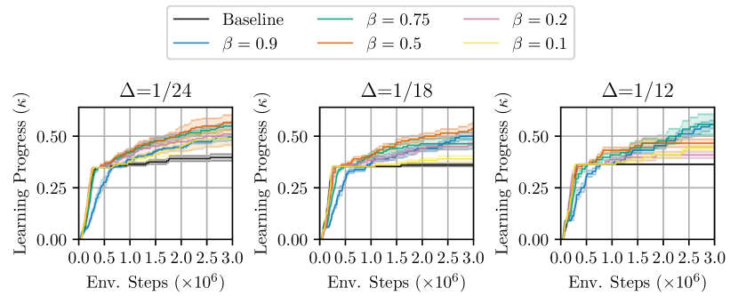
Refer to caption
(a) Vanilla Rollin without geometric sampling
Refer to caption
(b) Vanilla Rollin with geometric sampling
Figure 6: Vanilla Goal reaching. Accelerating learning on antmaze-umaze with Rollin on an oracle curriculum in Figure 3. The confidence interval represents the standard error computed over 8 random seeds.
Refer to caption
(a) Rollin + relabeling without geometric sampling
Refer to caption
(b) Rollin + relabeling with geometric sampling
Figure 7: Goal relabeling. Accelerating learning on antmaze-umaze with Rollin on an oracle curriculum in Figure 3. The confidence interval represents the standard error computed over 8 random seeds.
Refer to caption
(a) Rollin + Go-Explore without geometric sampling
Refer to caption
(b) Rollin + Go-Explore with geometric sampling
Figure 8: Go-Explore (exploration noise = 0.1). Accelerating learning on antmaze-umaze with Rollin on an oracle curriculum in Figure 3. The confidence interval represents the standard error computed over 8 random seeds.
Refer to caption
(a) Rollin + Go-Explore without geometric sampling
Refer to caption
(b) Rollin + Go-Explore with geometric sampling
Figure 9: Go-Explore (exploration noise = 0.25). Accelerating learning on antmaze-umaze with Rollin on an oracle curriculum in Figure 3. The confidence interval represents the standard error computed over 8 random seeds.
Refer to caption
(a) Rollin + Go-Explore without geometric sampling
Refer to caption
(b) Rollin + Go-Explore with geometric sampling
Figure 10: Go-Explore (exploration noise = 0.5). Accelerating learning on antmaze-umaze with Rollin on an oracle curriculum in Figure 3. The confidence interval represents the standard error computed over 8 random seeds.
Geo ΔΔ\Delta Baseline β=0.1𝛽0.1\beta=0.1 β=0.2𝛽0.2\beta=0.2 β=0.5𝛽0.5\beta=0.5 β=0.75𝛽0.75\beta=0.75 β=0.9𝛽0.9\beta=0.9
1/241241/24 0.40±0.02plus-or-minus0.400.020.40\pm 0.02 0.49±0.04plus-or-minus0.490.040.49\pm 0.04 0.51±0.05plus-or-minus0.510.050.51\pm 0.05 0.57±0.04plus-or-minus0.570.04\mathbf{0.57\pm 0.04} 0.55±0.02plus-or-minus0.550.020.55\pm 0.02 0.49±0.02plus-or-minus0.490.020.49\pm 0.02
1/181181/18 0.36±0.01plus-or-minus0.360.010.36\pm 0.01 0.39±0.01plus-or-minus0.390.010.39\pm 0.01 0.46±0.01plus-or-minus0.460.010.46\pm 0.01 0.54±0.03plus-or-minus0.540.03\mathbf{0.54\pm 0.03} 0.46±0.03plus-or-minus0.460.030.46\pm 0.03 0.50±0.02plus-or-minus0.500.020.50\pm 0.02
1/121121/12 0.36±0.00plus-or-minus0.360.000.36\pm 0.00 0.44±0.01plus-or-minus0.440.010.44\pm 0.01 0.41±0.02plus-or-minus0.410.020.41\pm 0.02 0.47±0.02plus-or-minus0.470.020.47\pm 0.02 0.56±0.05plus-or-minus0.560.05\mathbf{0.56\pm 0.05} 0.56±0.02plus-or-minus0.560.02\mathbf{0.56\pm 0.02}
1/241241/24 0.82±0.08plus-or-minus0.820.080.82\pm 0.08 0.92±0.02plus-or-minus0.920.020.92\pm 0.02 0.95±0.02plus-or-minus0.950.02\mathbf{0.95\pm 0.02} 0.88±0.01plus-or-minus0.880.010.88\pm 0.01 0.81±0.01plus-or-minus0.810.010.81\pm 0.01 0.70±0.02plus-or-minus0.700.020.70\pm 0.02
1/181181/18 0.68±0.07plus-or-minus0.680.070.68\pm 0.07 0.74±0.07plus-or-minus0.740.070.74\pm 0.07 0.76±0.06plus-or-minus0.760.060.76\pm 0.06 0.78±0.03plus-or-minus0.780.03\mathbf{0.78\pm 0.03} 0.75±0.02plus-or-minus0.750.020.75\pm 0.02 0.72±0.02plus-or-minus0.720.020.72\pm 0.02
1/121121/12 0.38±0.03plus-or-minus0.380.030.38\pm 0.03 0.55±0.04plus-or-minus0.550.040.55\pm 0.04 0.55±0.04plus-or-minus0.550.040.55\pm 0.04 0.64±0.06plus-or-minus0.640.060.64\pm 0.06 0.69±0.06plus-or-minus0.690.06\mathbf{0.69\pm 0.06} 0.67±0.03plus-or-minus0.670.030.67\pm 0.03
Table 8: Vanilla Goal reaching. Learning progress κ𝜅\kappa at 3 million environment steps with varying β𝛽\beta and curriculum step size ΔΔ\Delta of vanilla goal reaching task. Geo indicates the usage of geometric sampling. Baseline corresponds to β=0𝛽0\beta=0, where no Rollin is used. The standard error is computed over 8 random seeds. We highlight the values that are larger than the baseline (β=0𝛽0\beta=0) in purple, and the largest value in bold font.
Geo ΔΔ\Delta β=0𝛽0\beta=0 β=0.1𝛽0.1\beta=0.1 β=0.2𝛽0.2\beta=0.2 β=0.5𝛽0.5\beta=0.5 β=0.75𝛽0.75\beta=0.75 β=0.9𝛽0.9\beta=0.9
1/241241/24 0.89±0.03plus-or-minus0.890.030.89\pm 0.03 0.91±0.03plus-or-minus0.910.03\mathbf{0.91\pm 0.03} 0.85±0.04plus-or-minus0.850.040.85\pm 0.04 0.86±0.02plus-or-minus0.860.020.86\pm 0.02 0.86±0.02plus-or-minus0.860.020.86\pm 0.02 0.80±0.02plus-or-minus0.800.020.80\pm 0.02
1/181181/18 0.76±0.03plus-or-minus0.760.030.76\pm 0.03 0.81±0.01plus-or-minus0.810.010.81\pm 0.01 0.85±0.04plus-or-minus0.850.04\mathbf{0.85\pm 0.04} 0.79±0.01plus-or-minus0.790.010.79\pm 0.01 0.84±0.03plus-or-minus0.840.030.84\pm 0.03 0.68±0.04plus-or-minus0.680.040.68\pm 0.04
1/121121/12 0.66±0.04plus-or-minus0.660.040.66\pm 0.04 0.74±0.01plus-or-minus0.740.01\mathbf{0.74\pm 0.01} 0.73±0.03plus-or-minus0.730.030.73\pm 0.03 0.66±0.06plus-or-minus0.660.060.66\pm 0.06 0.67±0.05plus-or-minus0.670.050.67\pm 0.05 0.69±0.03plus-or-minus0.690.030.69\pm 0.03
1/241241/24 0.76±0.02plus-or-minus0.760.020.76\pm 0.02 0.78±0.01plus-or-minus0.780.010.78\pm 0.01 0.78±0.03plus-or-minus0.780.030.78\pm 0.03 0.82±0.02plus-or-minus0.820.020.82\pm 0.02 0.87±0.02plus-or-minus0.870.02\mathbf{0.87\pm 0.02} 0.83±0.02plus-or-minus0.830.020.83\pm 0.02
1/181181/18 0.72±0.02plus-or-minus0.720.020.72\pm 0.02 0.76±0.01plus-or-minus0.760.010.76\pm 0.01 0.76±0.02plus-or-minus0.760.020.76\pm 0.02 0.78±0.04plus-or-minus0.780.040.78\pm 0.04 0.85±0.03plus-or-minus0.850.03\mathbf{0.85\pm 0.03} 0.81±0.01plus-or-minus0.810.010.81\pm 0.01
1/121121/12 0.72±0.03plus-or-minus0.720.030.72\pm 0.03 0.73±0.00plus-or-minus0.730.00\mathbf{0.73\pm 0.00} 0.73±0.00plus-or-minus0.730.00\mathbf{0.73\pm 0.00} 0.73±0.03plus-or-minus0.730.03\mathbf{0.73\pm 0.03} 0.69±0.04plus-or-minus0.690.040.69\pm 0.04 0.66±0.04plus-or-minus0.660.040.66\pm 0.04
Table 9: Goal relabeling. All other settings are the same as Table 8.
EN Geo ΔΔ\Delta β=0𝛽0\beta=0 β=0.1𝛽0.1\beta=0.1 β=0.2𝛽0.2\beta=0.2 β=0.5𝛽0.5\beta=0.5 β=0.75𝛽0.75\beta=0.75 β=0.9𝛽0.9\beta=0.9
0.1 ✗ 1/241241/24 0.37±0.02plus-or-minus0.370.020.37\pm 0.02 0.52±0.07plus-or-minus0.520.070.52\pm 0.07 0.54±0.06plus-or-minus0.540.06\mathbf{0.54\pm 0.06} 0.51±0.06plus-or-minus0.510.060.51\pm 0.06 0.39±0.02plus-or-minus0.390.020.39\pm 0.02 0.37±0.01plus-or-minus0.370.010.37\pm 0.01
0.1 ✗ 1/181181/18 0.38±0.01plus-or-minus0.380.010.38\pm 0.01 0.37±0.01plus-or-minus0.370.010.37\pm 0.01 0.36±0.01plus-or-minus0.360.010.36\pm 0.01 0.38±0.01plus-or-minus0.380.010.38\pm 0.01 0.38±0.01plus-or-minus0.380.010.38\pm 0.01 0.35±0.00plus-or-minus0.350.000.35\pm 0.00
0.1 ✗ 1/121121/12 0.38±0.01plus-or-minus0.380.010.38\pm 0.01 0.38±0.01plus-or-minus0.380.010.38\pm 0.01 0.36±0.00plus-or-minus0.360.000.36\pm 0.00 0.39±0.01plus-or-minus0.390.01\mathbf{0.39\pm 0.01} 0.36±0.00plus-or-minus0.360.000.36\pm 0.00 0.36±0.00plus-or-minus0.360.000.36\pm 0.00
0.1 ✓ 1/241241/24 0.82±0.07plus-or-minus0.820.070.82\pm 0.07 0.95±0.02plus-or-minus0.950.02\mathbf{0.95\pm 0.02} 0.91±0.02plus-or-minus0.910.02{0.91\pm 0.02} 0.92±0.02plus-or-minus0.920.02{0.92\pm 0.02} 0.71±0.02plus-or-minus0.710.02{0.71\pm 0.02} 0.45±0.01plus-or-minus0.450.01{0.45\pm 0.01}
0.1 ✓ 1/181181/18 0.57±0.09plus-or-minus0.570.090.57\pm 0.09 0.71±0.08plus-or-minus0.710.08\mathbf{0.71\pm 0.08} 0.65±0.07plus-or-minus0.650.07{0.65\pm 0.07} 0.63±0.07plus-or-minus0.630.07{0.63\pm 0.07} 0.62±0.02plus-or-minus0.620.02{0.62\pm 0.02} 0.43±0.01plus-or-minus0.430.01{0.43\pm 0.01}
0.1 ✓ 1/121121/12 0.42±0.03plus-or-minus0.420.030.42\pm 0.03 0.43±0.02plus-or-minus0.430.02{0.43\pm 0.02} 0.38±0.04plus-or-minus0.380.04{0.38\pm 0.04} 0.49±0.04plus-or-minus0.490.04\mathbf{0.49\pm 0.04} 0.45±0.02plus-or-minus0.450.02{0.45\pm 0.02} 0.39±0.01plus-or-minus0.390.01{0.39\pm 0.01}
0.25 ✗ 1/241241/24 0.38±0.02plus-or-minus0.380.02{0.38\pm 0.02} 0.49±0.06plus-or-minus0.490.06{0.49\pm 0.06} 0.48±0.05plus-or-minus0.480.05{0.48\pm 0.05} 0.55±0.07plus-or-minus0.550.07\mathbf{0.55\pm 0.07} 0.43±0.04plus-or-minus0.430.04{0.43\pm 0.04} 0.40±0.02plus-or-minus0.400.02{0.40\pm 0.02}
0.25 ✗ 1/181181/18 0.35±0.00plus-or-minus0.350.00{0.35\pm 0.00} 0.39±0.03plus-or-minus0.390.03\mathbf{0.39\pm 0.03} 0.39±0.02plus-or-minus0.390.02\mathbf{0.39\pm 0.02} 0.36±0.01plus-or-minus0.360.01{0.36\pm 0.01} 0.36±0.01plus-or-minus0.360.01{0.36\pm 0.01} 0.35±0.00plus-or-minus0.350.00{0.35\pm 0.00}
0.25 ✗ 1/121121/12 0.36±0.00plus-or-minus0.360.00{0.36\pm 0.00} 0.36±0.00plus-or-minus0.360.00{0.36\pm 0.00} 0.36±0.00plus-or-minus0.360.00{0.36\pm 0.00} 0.36±0.00plus-or-minus0.360.00{0.36\pm 0.00} 0.36±0.00plus-or-minus0.360.00{0.36\pm 0.00} 0.36±0.00plus-or-minus0.360.00{0.36\pm 0.00}
0.25 ✓ 1/241241/24 0.82±0.10plus-or-minus0.820.10{0.82\pm 0.10} 0.97±0.02plus-or-minus0.970.02{0.97\pm 0.02} 1.00±0.00plus-or-minus1.000.00\mathbf{1.00\pm 0.00} 0.94±0.02plus-or-minus0.940.02{0.94\pm 0.02} 0.77±0.02plus-or-minus0.770.02{0.77\pm 0.02} 0.49±0.02plus-or-minus0.490.02{0.49\pm 0.02}
0.25 ✓ 1/181181/18 0.64±0.10plus-or-minus0.640.10{0.64\pm 0.10} 0.70±0.07plus-or-minus0.700.07{0.70\pm 0.07} 0.79±0.07plus-or-minus0.790.07\mathbf{0.79\pm 0.07} 0.64±0.06plus-or-minus0.640.06{0.64\pm 0.06} 0.63±0.03plus-or-minus0.630.03{0.63\pm 0.03} 0.44±0.01plus-or-minus0.440.01{0.44\pm 0.01}
0.25 ✓ 1/121121/12 0.39±0.01plus-or-minus0.390.01{0.39\pm 0.01} 0.47±0.03plus-or-minus0.470.03\mathbf{0.47\pm 0.03} 0.45±0.02plus-or-minus0.450.02{0.45\pm 0.02} 0.47±0.03plus-or-minus0.470.03\mathbf{0.47\pm 0.03} 0.36±0.04plus-or-minus0.360.04{0.36\pm 0.04} 0.40±0.02plus-or-minus0.400.02{0.40\pm 0.02}
0.5 ✗ 1/241241/24 0.49±0.06plus-or-minus0.490.060.49\pm 0.06 0.60±0.08plus-or-minus0.600.08{0.60\pm 0.08} 0.66±0.08plus-or-minus0.660.08\mathbf{0.66\pm 0.08} 0.61±0.08plus-or-minus0.610.08{0.61\pm 0.08} 0.65±0.06plus-or-minus0.650.06{0.65\pm 0.06} 0.46±0.04plus-or-minus0.460.04{0.46\pm 0.04}
0.5 ✗ 1/181181/18 0.36±0.01plus-or-minus0.360.010.36\pm 0.01 0.41±0.02plus-or-minus0.410.02\mathbf{0.41\pm 0.02} 0.39±0.01plus-or-minus0.390.01{0.39\pm 0.01} 0.38±0.01plus-or-minus0.380.01{0.38\pm 0.01} 0.37±0.01plus-or-minus0.370.01{0.37\pm 0.01} 0.35±0.00plus-or-minus0.350.00{0.35\pm 0.00}
0.5 ✗ 1/121121/12 0.36±0.00plus-or-minus0.360.000.36\pm 0.00 0.38±0.01plus-or-minus0.380.01\mathbf{0.38\pm 0.01} 0.38±0.01plus-or-minus0.380.01\mathbf{0.38\pm 0.01} 0.36±0.00plus-or-minus0.360.00{0.36\pm 0.00} 0.38±0.01plus-or-minus0.380.01\mathbf{0.38\pm 0.01} 0.36±0.00plus-or-minus0.360.00{0.36\pm 0.00}
0.5 ✓ 1/241241/24 0.92±0.08plus-or-minus0.920.080.92\pm 0.08 1.00±0.00plus-or-minus1.000.00\mathbf{1.00\pm 0.00} 1.00±0.00plus-or-minus1.000.00\mathbf{1.00\pm 0.00} 1.00±0.00plus-or-minus1.000.00\mathbf{1.00\pm 0.00} 0.87±0.03plus-or-minus0.870.03{0.87\pm 0.03} 0.55±0.03plus-or-minus0.550.03{0.55\pm 0.03}
0.5 ✓ 1/181181/18 0.66±0.09plus-or-minus0.660.090.66\pm 0.09 0.71±0.08plus-or-minus0.710.08{0.71\pm 0.08} 0.80±0.08plus-or-minus0.800.08\mathbf{0.80\pm 0.08} 0.68±0.08plus-or-minus0.680.08{0.68\pm 0.08} 0.67±0.04plus-or-minus0.670.04{0.67\pm 0.04} 0.44±0.02plus-or-minus0.440.02{0.44\pm 0.02}
0.5 ✓ 1/121121/12 0.41±0.02plus-or-minus0.410.020.41\pm 0.02 0.44±0.04plus-or-minus0.440.04{0.44\pm 0.04} 0.43±0.03plus-or-minus0.430.03{0.43\pm 0.03} 0.50±0.04plus-or-minus0.500.04\mathbf{0.50\pm 0.04} 0.47±0.03plus-or-minus0.470.03{0.47\pm 0.03} 0.39±0.04plus-or-minus0.390.04{0.39\pm 0.04}
Table 10: Go-Explore with different exploration noise. EN represents the multiplier for the Gaussian exploration noise. All other settings are the same as Table 8.

G.2 Non Goal Reaching Tasks

Refer to captionRefer to captionRefer to captionRefer to caption
Figure 11: Accelerating learning on several non goal-reaching tasks. The confidence interval represents the standard error computed over 8 random seeds, for β=0.1𝛽0.1\beta=0.1.
Env. Step β=0𝛽0\beta=0 β=0.1𝛽0.1\beta=0.1 β=0.2𝛽0.2\beta=0.2 β=0.5𝛽0.5\beta=0.5 β=0.75𝛽0.75\beta=0.75
walker 0.5m 0.83±0.03plus-or-minus0.830.030.83\pm 0.03 0.79±0.04plus-or-minus0.790.040.79\pm 0.04 0.75±0.04plus-or-minus0.750.040.75\pm 0.04 0.78±0.05plus-or-minus0.780.050.78\pm 0.05 0.76±0.05plus-or-minus0.760.050.76\pm 0.05
1m 0.92±0.03plus-or-minus0.920.030.92\pm 0.03 0.94±0.03plus-or-minus0.940.03\mathbf{0.94\pm 0.03} 0.90±0.01plus-or-minus0.900.010.90\pm 0.01 0.92±0.04plus-or-minus0.920.040.92\pm 0.04 0.92±0.03plus-or-minus0.920.030.92\pm 0.03
hopper 0.5m 0.85±0.02plus-or-minus0.850.020.85\pm 0.02 0.82±0.03plus-or-minus0.820.03{0.82\pm 0.03} 0.83±0.02plus-or-minus0.830.020.83\pm 0.02 0.78±0.02plus-or-minus0.780.020.78\pm 0.02 0.75±0.02plus-or-minus0.750.020.75\pm 0.02
1m 0.88±0.01plus-or-minus0.880.010.88\pm 0.01 0.89±0.00plus-or-minus0.890.00\mathbf{0.89\pm 0.00} 0.89±0.03plus-or-minus0.890.03\mathbf{0.89\pm 0.03} 0.82±0.02plus-or-minus0.820.020.82\pm 0.02 0.81±0.02plus-or-minus0.810.020.81\pm 0.02
humanoid 0.5m 0.32±0.05plus-or-minus0.320.050.32\pm 0.05 0.36±0.04plus-or-minus0.360.04\mathbf{0.36\pm 0.04} 0.21±0.07plus-or-minus0.210.070.21\pm 0.07 0.33±0.04plus-or-minus0.330.04{0.33\pm 0.04} 0.14±0.06plus-or-minus0.140.06{0.14\pm 0.06}
1m 0.67±0.03plus-or-minus0.670.030.67\pm 0.03 0.69±0.06plus-or-minus0.690.060.69\pm 0.06 0.62±0.02plus-or-minus0.620.020.62\pm 0.02 0.76±0.03plus-or-minus0.760.03\mathbf{0.76\pm 0.03} 0.71±0.06plus-or-minus0.710.06{0.71\pm 0.06}
ant 0.5m 0.72±0.02plus-or-minus0.720.020.72\pm 0.02 0.82±0.06plus-or-minus0.820.06\mathbf{0.82\pm 0.06} 0.68±0.08plus-or-minus0.680.080.68\pm 0.08 0.64±0.05plus-or-minus0.640.050.64\pm 0.05 0.47±0.05plus-or-minus0.470.050.47\pm 0.05
1m 1.00±0.00plus-or-minus1.000.001.00\pm 0.00 1.00±0.00plus-or-minus1.000.001.00\pm 0.00 0.83±0.08plus-or-minus0.830.080.83\pm 0.08 0.86±0.06plus-or-minus0.860.060.86\pm 0.06 0.71±0.07plus-or-minus0.710.07{0.71\pm 0.07}
Table 11: Learning progress κ𝜅\kappa at 0.5 and 1.0 million environment steps with varying β𝛽\beta of non goal reaching tasks. Baseline corresponds to β=0𝛽0\beta=0, where no Rollin is used. The standard error is computed over 8 random seeds. We highlight the values that are larger than the baseline (β=0𝛽0\beta=0) in purple, and the largest value in bold font.
Env. Step β=0𝛽0\beta=0 β=0.1𝛽0.1\beta=0.1 β=0.2𝛽0.2\beta=0.2 β=0.5𝛽0.5\beta=0.5 β=0.75𝛽0.75\beta=0.75
walker 0.5m 3.09±0.31plus-or-minus3.090.313.09\pm 0.31 2.83±0.31plus-or-minus2.830.31{2.83\pm 0.31} 2.41±0.33plus-or-minus2.410.332.41\pm 0.33 2.77±0.31plus-or-minus2.770.312.77\pm 0.31 2.88±0.32plus-or-minus2.880.322.88\pm 0.32
1m 3.69±0.27plus-or-minus3.690.273.69\pm 0.27 3.62±0.26plus-or-minus3.620.26{3.62\pm 0.26} 3.09±0.28plus-or-minus3.090.283.09\pm 0.28 3.48±0.27plus-or-minus3.480.273.48\pm 0.27 3.14±0.34plus-or-minus3.140.343.14\pm 0.34
hopper 0.5m 2.42±0.18plus-or-minus2.420.182.42\pm 0.18 2.26±0.22plus-or-minus2.260.22{2.26\pm 0.22} 2.45±0.14plus-or-minus2.450.14\mathbf{2.45\pm 0.14} 2.34±0.16plus-or-minus2.340.162.34\pm 0.16 2.34±0.16plus-or-minus2.340.16{2.34\pm 0.16}
1m 2.58±0.16plus-or-minus2.580.162.58\pm 0.16 2.65±0.15plus-or-minus2.650.15\mathbf{2.65\pm 0.15} 2.65±0.17plus-or-minus2.650.17\mathbf{2.65\pm 0.17} 2.39±0.18plus-or-minus2.390.182.39\pm 0.18 2.52±0.19plus-or-minus2.520.192.52\pm 0.19
humanoid 0.5m 0.26±0.05plus-or-minus0.260.050.26\pm 0.05 0.32±0.07plus-or-minus0.320.070.32\pm 0.07 0.27±0.05plus-or-minus0.270.050.27\pm 0.05 0.34±0.05plus-or-minus0.340.05{0.34\pm 0.05} 0.38±0.07plus-or-minus0.380.07\mathbf{0.38\pm 0.07}
1m 0.39±0.05plus-or-minus0.390.050.39\pm 0.05 0.46±0.09plus-or-minus0.460.090.46\pm 0.09 0.41±0.05plus-or-minus0.410.050.41\pm 0.05 0.41±0.06plus-or-minus0.410.06{0.41\pm 0.06} 0.49±0.10plus-or-minus0.490.10\mathbf{0.49\pm 0.10}
ant 0.5m 3.38±0.43plus-or-minus3.380.433.38\pm 0.43 3.85±0.41plus-or-minus3.850.41\mathbf{3.85\pm 0.41} 3.43±0.53plus-or-minus3.430.533.43\pm 0.53 3.15±0.45plus-or-minus3.150.453.15\pm 0.45 2.38±0.46plus-or-minus2.380.462.38\pm 0.46
1m 4.29±0.51plus-or-minus4.290.514.29\pm 0.51 4.66±0.30plus-or-minus4.660.30\mathbf{4.66\pm 0.30} 3.93±0.45plus-or-minus3.930.453.93\pm 0.45 3.99±0.48plus-or-minus3.990.483.99\pm 0.48 3.50±0.49plus-or-minus3.500.49{3.50\pm 0.49}
Table 12: Average x𝑥x-direction velocity of the last 50k time steps, at 0.5 and 1.0 million environment steps with varying β𝛽\beta of non goal reaching tasks. Baseline corresponds to β=0𝛽0\beta=0, where no Rollin is used. The standard error is computed over 8 random seeds. We highlight the values that are larger than the baseline (β=0𝛽0\beta=0) in purple, and the largest value in bold font.
Env. Step β=0𝛽0\beta=0 β=0.1𝛽0.1\beta=0.1 β=0.2𝛽0.2\beta=0.2 β=0.5𝛽0.5\beta=0.5 β=0.75𝛽0.75\beta=0.75
walker 0.5m 3450.1±307.4plus-or-minus3450.1307.43450.1\pm 307.4 3350.4±184.6plus-or-minus3350.4184.6{3350.4\pm 184.6} 2897.4±276.5plus-or-minus2897.4276.52897.4\pm 276.5 3255.9±203.8plus-or-minus3255.9203.83255.9\pm 203.8 3185.8±341.5plus-or-minus3185.8341.53185.8\pm 341.5
1m 4032.3±224.3plus-or-minus4032.3224.34032.3\pm 224.3 4128.8±159.6plus-or-minus4128.8159.6\mathbf{4128.8\pm 159.6} 3685.5±135.6plus-or-minus3685.5135.63685.5\pm 135.6 4028.8±164.2plus-or-minus4028.8164.24028.8\pm 164.2 3895.4±265.4plus-or-minus3895.4265.43895.4\pm 265.4
hopper 0.5m 3192.5±80.4plus-or-minus3192.580.43192.5\pm 80.4 3148.6±160.7plus-or-minus3148.6160.7{3148.6\pm 160.7} 3241.5±130.8plus-or-minus3241.5130.8\mathbf{3241.5\pm 130.8} 3116.5±141.8plus-or-minus3116.5141.83116.5\pm 141.8 3059.6±153.8plus-or-minus3059.6153.83059.6\pm 153.8
1m 3386.2±124.7plus-or-minus3386.2124.73386.2\pm 124.7 3421.9±109.8plus-or-minus3421.9109.8\mathbf{3421.9\pm 109.8} 3262.3±98.1plus-or-minus3262.398.1{3262.3\pm 98.1} 3170.7±180.6plus-or-minus3170.7180.63170.7\pm 180.6 3394.5±126.5plus-or-minus3394.5126.53394.5\pm 126.5
humanoid 0.5m 2910.1±262.9plus-or-minus2910.1262.92910.1\pm 262.9 2939.7±392.0plus-or-minus2939.7392.02939.7\pm 392.0 2598.9±309.8plus-or-minus2598.9309.82598.9\pm 309.8 3137.3±305.6plus-or-minus3137.3305.6\mathbf{3137.3\pm 305.6} 2259.6±245.4plus-or-minus2259.6245.4{2259.6\pm 245.4}
1m 3017.2±169.0plus-or-minus3017.2169.03017.2\pm 169.0 3173.6±238.3plus-or-minus3173.6238.33173.6\pm 238.3 2935.8±181.1plus-or-minus2935.8181.12935.8\pm 181.1 2905.5±125.9plus-or-minus2905.5125.9{2905.5\pm 125.9} 3290.7±275.9plus-or-minus3290.7275.9\mathbf{3290.7\pm 275.9}
ant 0.5m 2976.2±252.4plus-or-minus2976.2252.42976.2\pm 252.4 3593.1±237.8plus-or-minus3593.1237.8\mathbf{3593.1\pm 237.8} 3071.8±340.0plus-or-minus3071.8340.03071.8\pm 340.0 2818.3±265.2plus-or-minus2818.3265.22818.3\pm 265.2 2188.3±256.2plus-or-minus2188.3256.22188.3\pm 256.2
1m 4248.5±88.6plus-or-minus4248.588.64248.5\pm 88.6 4473.0±102.2plus-or-minus4473.0102.2\mathbf{4473.0\pm 102.2} 3683.1±345.0plus-or-minus3683.1345.03683.1\pm 345.0 3708.7±290.5plus-or-minus3708.7290.53708.7\pm 290.5 3250.1±316.2plus-or-minus3250.1316.2{3250.1\pm 316.2}
Table 13: Average return of the last 50k time steps, at the 0.5 and 1.0 million environment steps with varying β𝛽\beta of non goal reaching tasks. Baseline corresponds to β=0𝛽0\beta=0, where no Rollin is used. The standard error is computed over 8 random seeds. We highlight the values that are larger than the baseline (β=0𝛽0\beta=0) in purple, and the largest value in bold font.