Stein Variational Goal Generation for adaptive Exploration in Multi-Goal Reinforcement Learning
Abstract
In multi-goal Reinforcement Learning, an agent can share experience between related training tasks, resulting in better generalization for new tasks at test time. However, when the goal space has discontinuities and the reward is sparse, a majority of goals are difficult to reach. In this context, a curriculum over goals helps agents learn by adapting training tasks to their current capabilities. In this work we propose Stein Variational Goal Generation (svgg), which samples goals of intermediate difficulty for the agent, by leveraging a learned predictive model of its goal reaching capabilities. The distribution of goals is modeled with particles that are attracted in areas of appropriate difficulty using Stein Variational Gradient Descent. We show that svgg outperforms state-of-the-art multi-goal Reinforcement Learning methods in terms of success coverage in hard exploration problems, and demonstrate that it is endowed with a useful recovery property when the environment changes.
1 Introduction
Multi-goal Reinforcement Learning (RL) (Kaelbling, 1993), where agent policies are conditioned by goals specified according to the task at hand, has recently been at the heart of many research works (Schaul et al., 2015; Pitis et al., 2020; Yang et al., 2021), since it offers an efficient way for sharing experience between related tasks. The usual ambition in the multi-goal RL context is to obtain an agent able to reach any goal from some desired goal distribution. This is particularly challenging in settings where the desired goal distribution is unknown at train time, which means discovering the space of valid goals by experience, and optimizing success coverage111Success coverage, which measures the average performance of the agent on all valid goals, is denoted competence in (Blaes et al., 2019).
To avoid deceptive gradient issues and a tedious reward engineering process, multi-goal RL often considers the sparse reward context, where the agent only obtains a non-null learning signal when the goal is achieved. In that case, the multi-goal framework makes it possible to leverage Hindsight Experience Replay (her) (Andrychowicz et al., 2017) which helps densify the reward signal by relabeling failures as successes for the goals achieved by accident. However, in settings with discontinuities in the goal space (e.g., walls in a maze), or in hard exploration problems where the long task horizon results in an exponential decrease of the learning signal (Osband et al., 2016), many goals remain hard to achieve and using her does not suffice to reach all valid goals. In these more difficult contexts, and without any desired goal distribution at hand, the selection of training goals from a behavior distribution must be structured into a curriculum to help agents explore and learn progressively by adapting training tasks to their current capabilities (Colas et al., 2022). The question is: how can we organize a curriculum of goals to maximize the success coverage?
A first approach consists in focusing on novelty, with the objective of expanding the set of achieved goals. This is the approach of rig (Nair et al., 2018), discern (Warde-Farley et al., 2018), Skew-Fit (Pong et al., 2019) and mega (Pitis et al., 2020)222This is also the case for omega (Pitis et al., 2020), which extends mega, but for settings where the desired goal distribution is known, which leaves the scope of our work.. This leads to strong exploration results, but success coverage is only optimized implicitly.
Another strategy is to bias the goal generation process toward goals of intermediate difficulty (GOIDs). The general intuition is that addressing goals that are too easy or too hard does not foster progress, thus the agent needs to identify goals on which it can make some progress. The focus is thus more on performance. This is the approach of asymetric self-play (Sukhbaatar et al., 2017), Goal gan (Florensa et al., 2018), setter-solver (Racaniere et al., 2019) or vds (Zhang et al., 2020). By aiming at performance, those methods target more explicitly success in encountered goals, but benefit from implicit exploration.
In this work, we propose a novel method which provides the best of both worlds. Our method, called svgg 333For Stein Variational Goal Generation., learns a model of the probability of succeeding in achieving goals by relying on a set of particles where each particle represents a goal candidate. This set of particles is updated via Stein Variational Gradient Descent (Liu & Wang, 2016) to fit GOIDs, modeled as goals whose success is the most unpredictable. A key feature of svgd is that the gradient applied to particles combines an attraction term and a repulsion term, which helps strike a good balance between exploration and exploitation. In particular, when the agent cannot find any additional GOID, due to the repulsion term of svgd, the current particles repel one another resulting in fostering more exploratory goal sampling. This endows svgg with a very flexible model of the current capabilities of the corresponding agent. Based on this feature, we formally demonstrate that svgg possesses a very useful recovery property that prevents catastrophic forgetting and enables the agent to adapt when the environment changes during training. We empirically validate svgg on Multi-goal RL problems where the goal space is of moderate size, and leave investigations on problems where goals are images for future work.
2 Background
2.1 Goal-conditioned Reinforcement Learning
In this paper, we consider the multi-goal reinforcement learning setting, defined as a Markov Decision Process (MDP) , where is a set of states, is the set of transitions, the set of actions and the reward function is parametrized by a goal lying in the d-dimensional continuous goal space . In our setting, each goal is defined as a set of states that are desirable situations for the corresponding task, with states in being terminal states of the corresponding MDP. Thus, a goal is considered achieved when the agent reaches at step any state , which implies the following sparse reward function in the absence of expert knowledge. The goal-conditioned reward function is defined as for discrete state spaces and for discrete ones, where is a distance threshold and the indicator function.
Then, the objective is to learn a goal-conditioned policy (GCP) which maximizes the expected cumulative reward from any initial state of the environment, given a goal : , where stands for the goal-conditioned reward obtained at step of trajectory using goal , is a discount factor in and is the distribution of goals over . In our setting we consider that is uniform over (i.e., no known desired distribution), while the work could be extended to cover different distributions.
Importantly, since is not known in advance and we want to adapt training goals to the current capabilities of the agent, learning is performed at each step through goals sampled from a behavioral distribution , which is periodically updated by experience. While training the agent can be performed by any classical RL algorithm, our work focuses on the definition of this behavioral distribution , which drives the learning process.
2.2 Automatic Curriculum for sparse Reward RL
Our svgg method addresses automatic curriculum for sparse reward goal-conditioned RL (GCRL) problems and learns to achieve a continuum of related tasks.
Achieved Goals Distributions
Our work is strongly related to the mega algorithm (Pitis et al., 2020), which (1) maintains a buffer of previously achieved goals, (2) models the distribution of achieved goals via a kernel density estimation (KDE), and (3) uses this distribution to define its behavior distribution. By preferably sampling from the buffer goals at the boundary of the set of already reached states, an increase of the support of that distribution is expected. In that way, mega aims at overcoming the limitations of previous related approaches which also model the distribution of achieved goals. For instance, discern (Warde-Farley et al., 2018) only uses a replay buffer of goals whereas rig (Nair et al., 2018) and Skew-Fit (Pong et al., 2019) rather use variational auto-encoding (Kingma & Welling, 2013) of the distribution. While rig samples from the model of the achieved distribution, and discern and Skew-Fit skew that distribution to sample more diverse achieved goals, mega rather focuses on low density regions of the distribution, aiming to expand it. This results in improved exploration compared to competitors. Our approach differs from all these works as they only model achieved goals, independently from which goal was targeted when they were achieved, whereas we model the capability of reaching target goals. This makes a strong difference since, while mega selects goals at the frontier of what it already discovered, nothing indicates that goals closer to the mode of the distribution can be achieved when they are targeted. mega is also prone to catastrophic forgetting and limits exploration to goals present in the replay buffer.
Adversarial Goal Generation
Another trend proposes to adversarially learn a goal generator, that produces targets that are at the frontier of the agent’s capabilities. In that vein, Goal gan (Florensa et al., 2018) simultaneously learns a discriminator to sort out non GOIDs or generated goals from GOIDs in the buffer of achieved goals, and a generator that aims at producing goals that fool the discriminator. While appealing, the approach is prone to instabilities, with a generator that may usually diverge far from the space of reachable goals. setter-solver (Racaniere et al., 2019) stands as an extension of Goal gan, where a goal setter is learned to provide goals of various levels of difficulty w.r.t. a judge network (similar to our success predictor, see next section). The provided goals remain close to already achieved goals, and are diverse enough to avoid mode collapse. This approach however suffers from relying on invertible networks to map from the latent space to the goal space, which severely limits the modeling power, and can reveal problematic for environments with strong discontinuities. Asymmetric self-play (Sukhbaatar et al., 2017) is another way to generate goals, with a teacher agent seeking to produce goals that are just beyond the capabilities of the student agent. Both teacher and student learn simultaneously, with an equilibrium of adverse rewards determined on their respective time to go. However, this balance is hard to maintain, and many useful areas are usually missed. Our svgg algorithm also samples GOIDs, but it does so by learning a predictive model of the agent’s goal achievement capability and building a sampling distribution that focuses on goals whose achievement is the most unpredictable. Because it does not call upon an adversarial generative process, svgg is less prone to instabilities.
2.3 Stein Variational Gradient Descent
Our method builds on Stein Variational Gradient Descent (svgd) (Liu & Wang, 2016) to approximate the distribution of goals of interest. svgd is a powerful non-parametric tool for density estimation, when the partition function of the target distribution to approximate is intractable, which is the case when we do not know the support of the valid goal distribution in the environment. It stands as an efficient alternative to MCMC methods, which are proven to converge to the true distribution but are usually too slow to be used in complex optimization processes. It also stands as an alternative to variational inference of parametric neural distributions , which are restricted to pre-specified families of distributions (e.g., Gaussian or mixtures of Gaussians) that may not fit target distributions. Instead, it models as a set of particles , all belonging to the support of .
The idea behind svgd is to approximate the target distribution with by minimizing their KL-divergence: . This objective is reached by iterative deterministic transforms as small perturbations of the identity map, on the set of particles: , where is a smooth transform function that indicates the direction of the perturbation, while is the magnitude.
The authors draw a connection between KL-divergence and the Stein operator by showing that , where is the distribution of particles after the transformation . The KL minimization objective is thus related to the Stein Discrepancy, defined as: 444Note that only if ..
Minimizing Stein Discrepancy being intractable as such, (Liu et al., 2016) and (Chwialkowski et al., 2016) introduce the Kernelized Stein Discrepancy (KSD) where the idea is to restrict to projections that belong to the unit ball of a reproducing kernel Hilbert space (RKHS), for which there is a closed form solution. The KSD is defined as , whose solution is given by: , where is the positive definite kernel of the RKHS . The RBF kernel is commonly used.
Therefore, the steepest descent on the KL-objective is given by the optimal transform , where
| (1) |
The “attractive force” in the update 1 drives the particles toward high density areas of the target . The “repulsive force” pushes the particles away from each other, therefore fosters exploration and avoids mode collapse. Note that if , the update in (1) corresponds to a Maximum a Posteriori.
svgd has already been successfully explored in the context of RL. The Stein Variational Policy Gradient (svpg) (Liu et al., 2017) employs svgd to maintain a distribution of efficient agents as particles. It strongly differs from our approach, since we consider particles as behavior goal candidates, while svpg aims at capturing the epistemic uncertainty about policy parameters. (Chen et al., 2021) also relies on svgd to build a strategy to generate goals to agents, but in a very simplified setting without the attractive force from (1), which prevents from fully benefiting from this theoretical framework. Notably, such a kind of approach is particularly sensitive to catastrophic forgetting.
3 Stein Variational Goal Generation
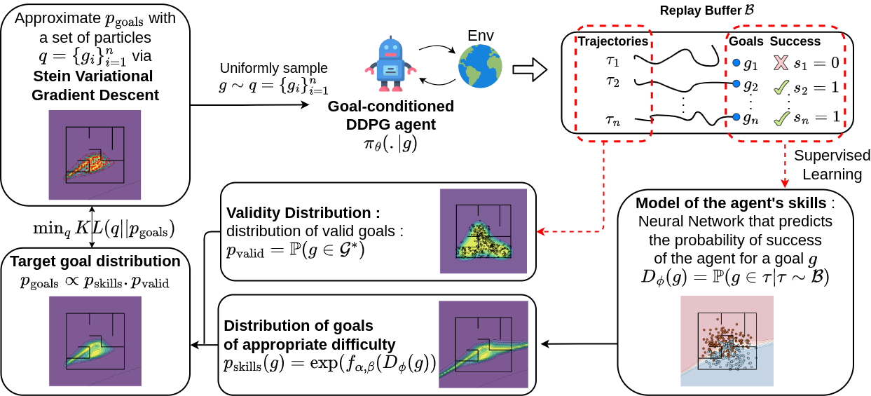
In this section we introduce our Stein Variational Goal Generation (svgg) algorithm. The pseudo-code of svgg is given in Algorithm 1 (a more detailed version is given in Appendix G.2). Our aim is to obtain a curriculum to sample goals of appropriate difficulty for the RL agent, where the curriculum is represented as an evolving goal sampling probability . To do so, we maintain a model of the agent’s skills – or goal reaching capability –, which helps define a distribution . This distribution assigns probability mass to areas of goals of appropriate difficulty. Additionally, with a simple one class SVM, we learn a validity distribution preventing the particles from being sampled from non-valid areas of the goal space. Then, we aim at sampling training goals from the following target distribution:
| (2) |
Since computing the partition function is intractable for such a distribution formulation, we rather sample uniformly over a set of particles , that are optimized through SVGD to approximate . Importantly, for our setting where we are interested in tracking useful areas to train the agent, dealing with a set of particles representing the state of the full exploration landscape appears better fitted than methods relying on single candidates, such as MCMC or Langevin Dynamics, that would produce samples very correlated in time, with unstable dynamics. This choice also improves the interpretability of the process, by providing a comprehensive picture of the current behavior distribution along training. Formal definitions of the two components of are given below.
Model of the agent’s skills
The probability is modeled as a Neural Network whose parameters are learned by gradient descent on the following Binary Cross Entropy (BCE) loss:
| (3) |
where is a batch of pairs coming from recent trajectories of the agent in the environment. The sampled goals are those whose predicted probability of success is neither too high nor too low (i.e., we avoid or ).
To build based on the prediction of , we use a beta distribution whose maximum density point mass is determined according to the output of , by two hyper-parameters and that shape the distribution and control the difficulty of the addressed goals, as illustrated on Figure 7 in appendix.
We define the distribution as an energy-based density whose potential is the output of the beta distribution :
| (4) |
In Appendix D, we compare the relative performance of 5 pairs of and and show that target a Medium difficulty works best. We stick to this setting in the rest of the study.
Validity distribution
As outlined in (Racaniere et al., 2019), we would like to only sample valid goals. To do so, instead of their validity loss, we define a validity distribution which represents the probability that a goal belongs to the set of valid (reachable) goals . However, is not known in advance. To circumvent this difficulty, the states already reached by the agent are stored in an archive and we aim at defining the validity distribution as depending on the posterior probability given : . We progressively build this distribution with a One Class SVM (OCSVM). This model is mainly designed for outlier or novelty detection in absence of labeled data. Given a dataset , it defines a boundary of the data support in , while keeping a small portion of the data points out of that boundary. With data points being goals from , we get
| (5) |
where is the output of the OCSVM model trained on , with parameters . As the agent progresses and expands its set of achieved states through training, it eventually reaches the environment boundary. In this case, we can expect for any area .
Recovery property
As demonstrated in Theorem 1 and empirically validated in Section 4.2, svgg benefits from a useful recovery property: when the environment suddenly changes, the svgg agent will spontaneously resample goals in the areas that are affected by the change.
Theorem 1.
Recovery property: Let us denote as the set of goals such that and its convex hull. Assume that, at a given iteration , for every (i.e., the whole set is considered as mastered by ), and that, on that set, is well calibrated: for any area and any goal , . Assume also that we use a kernel which ensures that the Kernelized Stein Discrepancy of any distribution with is 0 only if weakly converges to 555As assumed for instance in (Liu, 2017). This is not always true, but gives strong insights about the behavior of svgd. Refer to (Gorham & Mackey, 2017) for more discussions about KSD.. Then, with no updates of the models after iteration and a number of particles , any area with diameter eventually contains at least one particle, whenever after convergence of the particle updates.
The above theorem (proof in Appendix A) ensures that, even if the success model overestimates the capacities of the agent for some area (e.g., due to changes in the environment, catastrophic forgetting or success model error), some particles are likely to go back to this area once every goal in looks well covered by the agent, with an increasing probability for more particles. This way, the process can reconsider overestimated areas, by sampling again goals in them, and hence correcting the corresponding predictions, which leads to attracting attention of back to these difficult areas. Approaches such as mega do not exhibit such recovery properties, since they always sample at the boundary of their achievable goal distribution, which is likely to incrementally grow towards . The particles of our approach can be seen as attention trackers which remodel the behavior distribution and mobilize the effort on useful areas when needed. This is much better than uniformly sampling from the whole space of achievable states with small probability, which would also ensure some recovery of forgotten areas but in a very inefficient way. This theoretical guarantee of svgg is empirically validated by the experiment from Figure 3, which shows the good recovery property of our approach, after a sudden change in the environment.
4 Experiments
4.1 Experimental setup
Success coverage metric
Our general objective is to obtain a policy that can reliably achieve all valid goals in some environment. To quantify this objective, we evaluate the resulting policy on the entire space of valid goals in our environment using a success coverage metric, defined as , with the volume of . The goal space being continuous, we evaluate the policy on a finite subset uniformly sampled from . Then our objective reduces to:
| (6) |
To build , we split into areas following a regular grid, and then uniformly sample 30 goals inside each part of the division.
Compared Approaches
As baselines, we choose two methods from the literature that span the existing trends in unsupervised RL with goal-conditioned policies, mega (Pitis et al., 2020) and Goal gan (Florensa et al., 2018). In addition, the Random baseline randomly selects the behavior goal among past achieved states.
We also evaluate two svgg ablations: a No Validity Distribution version, which considers and a Only Validity version, where .
Learning to reliably achieve all valid goals can be decomposed in learning to sample appropriate behavioral goals, and learning to achieve these goals. Our focus being on the goal sampling mechanism, all compared approaches learn to achieve goals using ddpg and her with a mixed strategy described in Appendix G. In all versions of svgg, we use particles to approximate the target distribution. Implementation details about all considered architectures are given in Appendix G.
Questions
To compare the performance of svgg to baselines, we investigate the following questions: 1) Does svgg maximize the success coverage metric better than the baselines? 3) Is svgg more robust than the baselines to catastrophic forgetting that may occur in sudden environment changes? In Appendix D, we also investigate the impact of target difficulty (i.e., beta distribution as described above) on success coverage maximization.
Evaluation environments
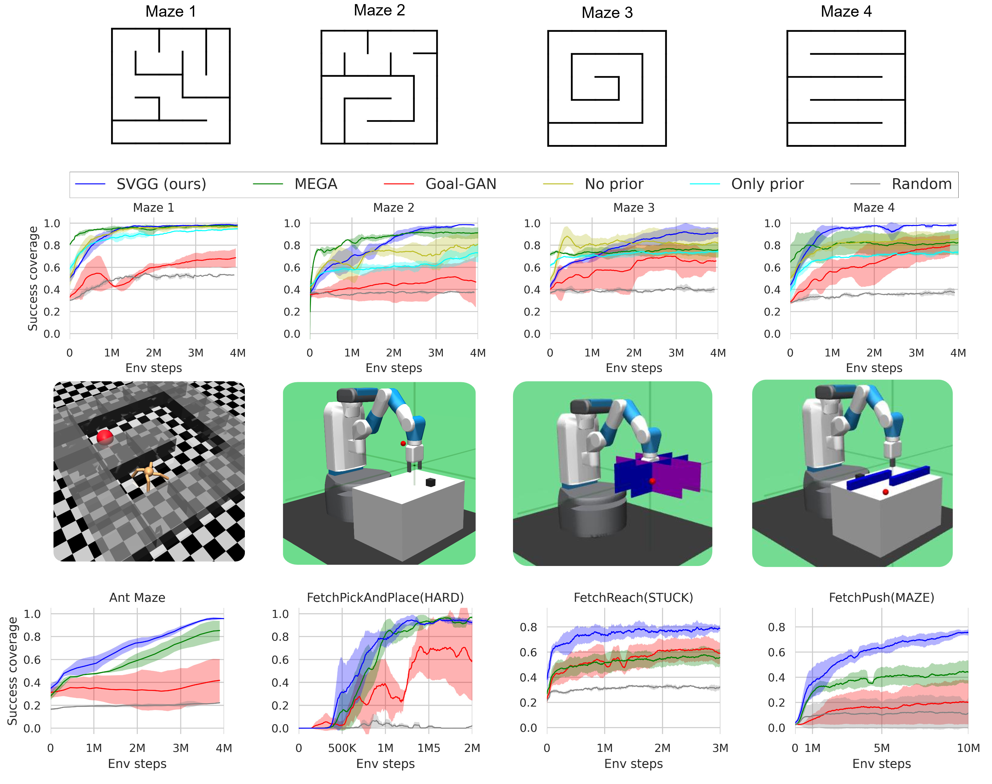
To answer the above metric-oriented questions, we use a modified version of the FetchReach and FetchPush environments (Plappert et al., 2018) where we have added obstacles in the workspace of the robot arm to increase the amount of discontinuities between the optimal goal-oriented behaviors. We also compare svgg to baselines in the U-shaped AntMaze environment (Trott et al., 2019) and in a hard version of FetchPickAndPlace. Additionally, to provide more analysis-oriented visualizations, we use a Point-Maze environment where an agent moves a point without mass within a 2D maze with continuous spaces of states and actions. As the agent does not perceive the walls, maximizing success coverage in these environments is harder than it seems.
4.2 Main results
Success coverage evaluations
Figure 2 shows that svgg significantly outperforms all baselines in terms of success coverage. Especially in highly discontinuous goal space settings such as in mazes and the modified version on FetchReach and FetchPush, where it efficiently discovers and achieves most of the valid goals. On AntMaze and FetchPickAndPlace, where the goal space is more smooth, our approach obtains comparable results to its competitors.
Due to the known stability issues in GAN training, Goal gan is the least efficient baselines. Another explanation of the failure of Goal gan is that it is likely to generate non valid goals, which is not the case for mega or svgg. mega chooses behavior goals from a Replay Buffer of achieved goals, while the validity distribution considered in svgg keeps particles inside valid areas.
The minimum density heuristic of mega efficiently discovers all valid goals in the environment, but our results show that its success plateaus in almost all the considered environments. mega’s intrinsic motivation only relies on state novelty. Thus, when the agent has discovered all reachable states, it is unable to target areas that it has reached in the past but has not mastered yet.
Recovery Property
Figure 3 shows the advantages of svgg over mega and Goal gan in changing environments. Walls are suddenly added during the training process (dot black line from Figure 3), after the methods had reached their pick performance. We see that the performance of mega and Goal gan plateaus lower than their pick performance (see Figure 2) whereas svgg discovers new difficulties resulting from the environment modification and focuses on those to finally recover its pick success coverage.
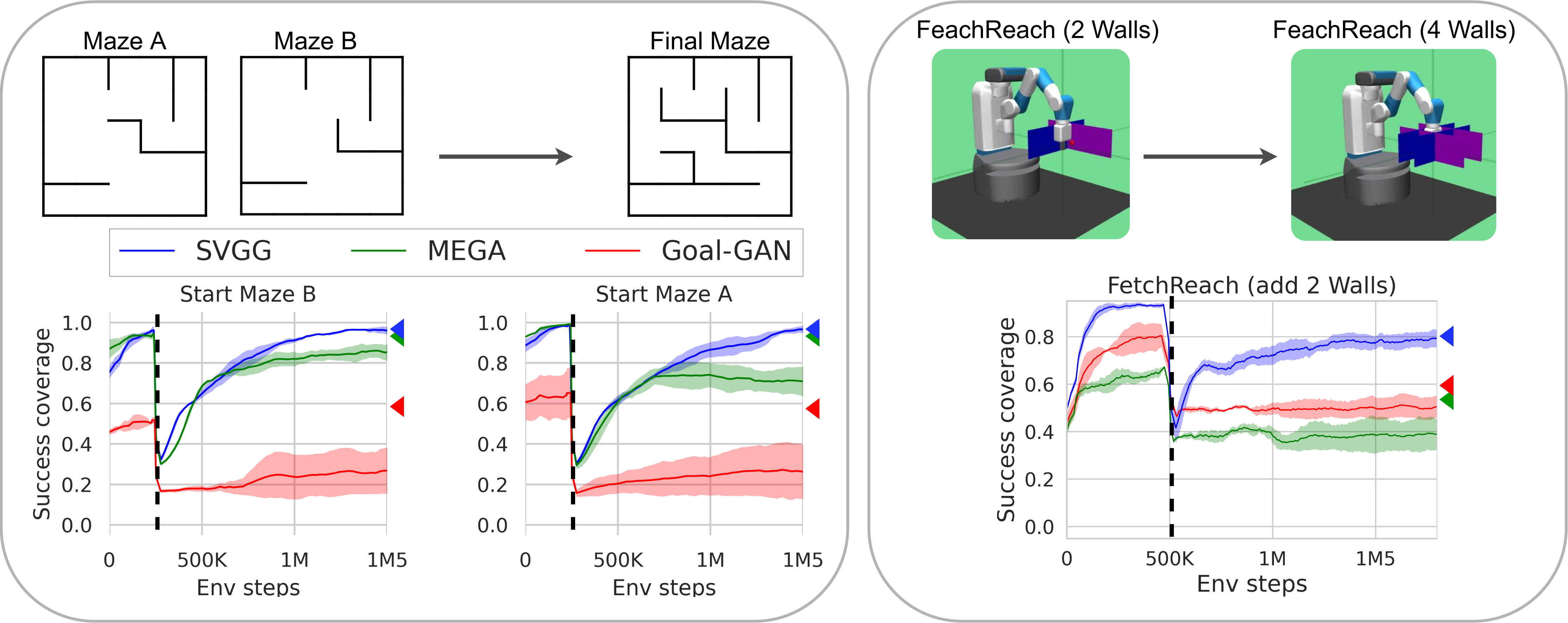
We also observe that the advantages of our method over mega in terms of recovery ability are more significant when changes in the environment are more drastic (i.e., when starting from maze B).
Further SVGG analyses
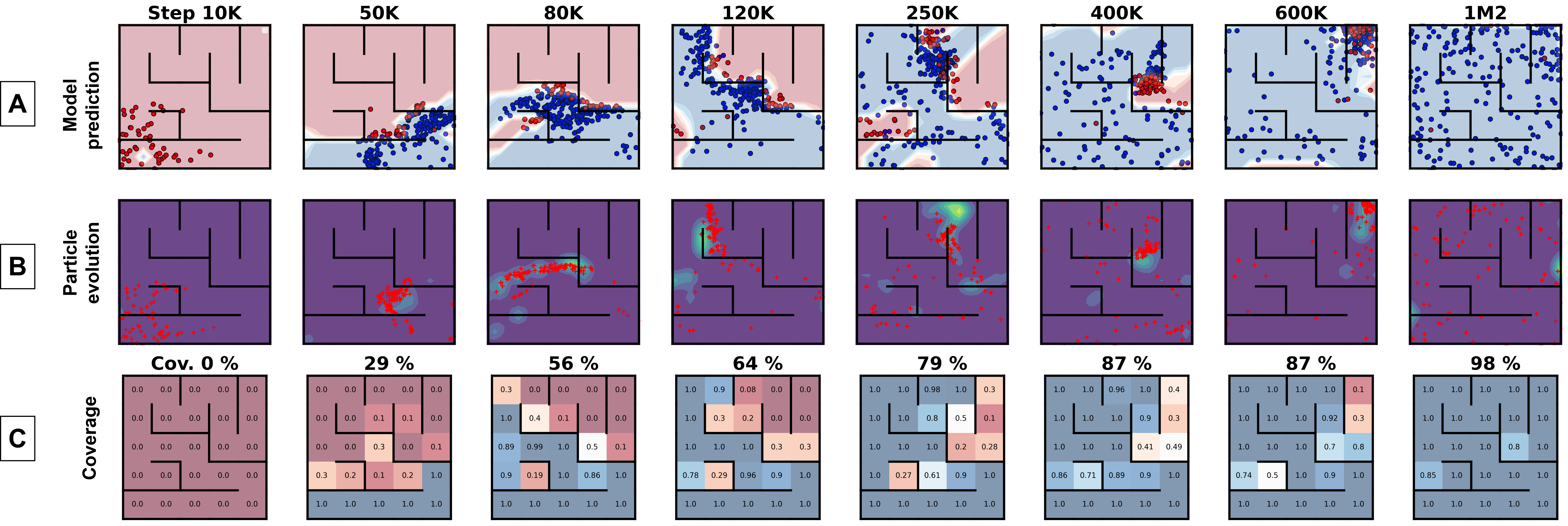
To gain further intuition on how svgg maximizes the success coverage, we show in Figure 4 the evolution of the particles throughout training. As the agent progresses and achieves novel and harder goals, the model updates its predictions. Thus, the target distribution is updated accordingly (background color of the row of the figure). The particles are then moved toward new areas of intermediate difficulty through svgd to minimize .
Figure 4 also highlights the recovery property of svgg. When the agent has nothing else to learn in the environment, reduces to , that is at this point uniform over the entire goal space. Therefore, the particles spread uniformly over the goal space and prevent svgg from catastrophic forgetting, as the model rediscovers areas that the agent has forgotten how to reach (cf. rightmost column in Figure 4). Additional analyses on svgg are given in Appendix D.
5 Conclusion
This paper introduces a new multi-goal reinforcement learning algorithm, svgg, which leverages Stein Variational Gradient Descent to monitor a model w.r.t. its goal achievement capabilities. Using this model, the agent addresses goals of intermediate difficulty, resulting in an efficient curriculum for finally covering the whole goal space. Moreover, svgg can recover from catastrophic forgetting, which is a classic pitfall in multi-goal RL.
Studying the impact of the number of particles is left for future work. Actually, the target distribution being in constant evolution, the KL divergence minimization objective is hard to reach at all times, which makes it difficult to claim that using more particles is always better. Furthermore, a previous work (D’Angelo & Fortuin, 2021) spotted exploration failures in svgd, and suggests that periodically annealing the attraction force in particle optimization (1) is required to enable particles to cover non-trivial distributions, e.g. in multimodal settings (which is the case for us) or in high dimensions.
Some limitations should be addressed in future work. The environments used in our experiments have low dimensional goal space, which facilitates the approximation of the target distribution with svgd and the agent’s model learning phase. When the agent’s observation and goal space will be images, the agent should learn a compact latent space of observation as in (Pong et al., 2019; Yarats et al., 2021; Liu & Abbeel, 2021; Hafner et al., 2019), using various representation learning techniques like contrastive learning, prototypical representations or variational auto-encoders. In future work, we should learn a latent goal space from observations, and perform svgd over particles in this latent space. This would result in an end-to-end algorithm learning to discover and achieve all possible goals in its environment from pixels.
Besides, we also envision to address larger and stochastic environments, where additional uncertainty estimation should be added to the goal generation process, to prevent the agent getting stuck in uncontrollable states (like a TV screen showing white noise) as in (Chua et al., 2018; Pathak et al., 2019), using methods such as model disagreement between multiple agents.
Acknowledgments
We thank our colleges at ISIR and the anonymous reviewers for their helpful comments. This work benefited from the use SCAI (Sorbonne Center for Artificial Intelligence) cluster of GPUs. This work has received funding from the European Commission’s Horizon Europe Framework Programme under grant agreement No 101070381 (PILLAR-robots project).
References
- Andrychowicz et al. (2017) Andrychowicz, M., Wolski, F., Ray, A., Schneider, J., Fong, R., Welinder, P., McGrew, B., Tobin, J., Abbeel, P., and Zaremba, W. Hindsight Experience Replay. arXiv preprint arXiv:1707.01495, 2017.
- Blaes et al. (2019) Blaes, S., Vlastelica Pogančić, M., Zhu, J., and Martius, G. Control what you can: Intrinsically motivated task-planning agent. Advances in Neural Information Processing Systems, 32, 2019.
- Brockman et al. (2016) Brockman, G., Cheung, V., Pettersson, L., Schneider, J., Schulman, J., Tang, J., and Zaremba, W. Openai gym, 2016.
- Chen et al. (2021) Chen, J., Zhang, Y., Xu, Y., Ma, H., Yang, H., Song, J., Wang, Y., and Wu, Y. Variational automatic curriculum learning for sparse-reward cooperative multi-agent problems, 2021. URL https://arxiv.org/abs/2111.04613.
- Chua et al. (2018) Chua, K., Calandra, R., McAllister, R., and Levine, S. Deep reinforcement learning in a handful of trials using probabilistic dynamics models, 2018. URL https://arxiv.org/abs/1805.12114.
- Chwialkowski et al. (2016) Chwialkowski, K., Strathmann, H., and Gretton, A. A kernel test of goodness of fit. In Balcan, M. F. and Weinberger, K. Q. (eds.), Proceedings of The 33rd International Conference on Machine Learning, volume 48 of Proceedings of Machine Learning Research, pp. 2606–2615, New York, New York, USA, 20–22 Jun 2016. PMLR. URL https://proceedings.mlr.press/v48/chwialkowski16.html.
- Colas et al. (2022) Colas, C., Karch, T., Sigaud, O., and Oudeyer, P.-Y. Autotelic agents with intrinsically motivated goal-conditioned reinforcement learning: a short survey. Journal of Artificial Intelligence Research, 74:1159–1199, 2022.
- D’Angelo & Fortuin (2021) D’Angelo, F. and Fortuin, V. Annealed stein variational gradient descent. CoRR, abs/2101.09815, 2021. URL https://arxiv.org/abs/2101.09815.
- Eysenbach et al. (2020) Eysenbach, B., Geng, X., Levine, S., and Salakhutdinov, R. Rewriting history with inverse RL: hindsight inference for policy improvement. CoRR, abs/2002.11089, 2020. URL https://arxiv.org/abs/2002.11089.
- Florensa et al. (2018) Florensa, C., Held, D., Geng, X., and Abbeel, P. Automatic goal generation for reinforcement learning agents. In International conference on machine learning, pp. 1515–1528. PMLR, 2018.
- Gorham & Mackey (2017) Gorham, J. and Mackey, L. Measuring sample quality with kernels. In International Conference on Machine Learning, pp. 1292–1301. PMLR, 2017.
- Hafner et al. (2019) Hafner, D., Lillicrap, T., Fischer, I., Villegas, R., Ha, D., Lee, H., and Davidson, J. Learning latent dynamics for planning from pixels. In Chaudhuri, K. and Salakhutdinov, R. (eds.), Proceedings of the 36th International Conference on Machine Learning, volume 97 of Proceedings of Machine Learning Research, pp. 2555–2565. PMLR, 09–15 Jun 2019. URL https://proceedings.mlr.press/v97/hafner19a.html.
- Kaelbling (1993) Kaelbling, L. P. Learning to achieve goals. In IJCAI, pp. 1094–1099. Citeseer, 1993.
- Kingma & Welling (2013) Kingma, D. P. and Welling, M. Auto-encoding variational bayes. arXiv preprint arXiv:1312.6114, 2013.
- Liu & Abbeel (2021) Liu, H. and Abbeel, P. Behavior from the void: Unsupervised active pre-training, 2021. URL https://arxiv.org/abs/2103.04551.
- Liu (2017) Liu, Q. Stein variational gradient descent as gradient flow. In Guyon, I., Luxburg, U. V., Bengio, S., Wallach, H., Fergus, R., Vishwanathan, S., and Garnett, R. (eds.), Advances in Neural Information Processing Systems, volume 30. Curran Associates, Inc., 2017. URL https://proceedings.neurips.cc/paper/2017/file/17ed8abedc255908be746d245e50263a-Paper.pdf.
- Liu & Wang (2016) Liu, Q. and Wang, D. Stein variational gradient descent: A general purpose bayesian inference algorithm. arXiv preprint arXiv:1608.04471, 2016.
- Liu et al. (2016) Liu, Q., Lee, J., and Jordan, M. A kernelized stein discrepancy for goodness-of-fit tests. In Balcan, M. F. and Weinberger, K. Q. (eds.), Proceedings of The 33rd International Conference on Machine Learning, volume 48 of Proceedings of Machine Learning Research, pp. 276–284, New York, New York, USA, 20–22 Jun 2016. PMLR. URL https://proceedings.mlr.press/v48/liub16.html.
- Liu et al. (2017) Liu, Y., Ramachandran, P., Liu, Q., and Peng, J. Stein variational policy gradient. arXiv preprint arXiv:1704.02399, 2017.
- Nair et al. (2018) Nair, A., Pong, V., Dalal, M., Bahl, S., Lin, S., and Levine, S. Visual reinforcement learning with imagined goals. arXiv preprint arXiv:1807.04742, 2018.
- Osband et al. (2016) Osband, I., Van Roy, B., and Wen, Z. Generalization and exploration via randomized value functions. In International Conference on Machine Learning, pp. 2377–2386. PMLR, 2016.
- Pathak et al. (2019) Pathak, D., Gandhi, D., and Gupta, A. Self-supervised exploration via disagreement, 2019. URL https://arxiv.org/abs/1906.04161.
- Pitis et al. (2020) Pitis, S., Chan, H., Zhao, S., Stadie, B., and Ba, J. Maximum entropy gain exploration for long horizon multi-goal reinforcement learning. In III, H. D. and Singh, A. (eds.), Proceedings of the 37th International Conference on Machine Learning, volume 119 of Proceedings of Machine Learning Research, pp. 7750–7761. PMLR, 13–18 Jul 2020. URL https://proceedings.mlr.press/v119/pitis20a.html.
- Plappert et al. (2018) Plappert, M., Andrychowicz, M., Ray, A., McGrew, B., Baker, B., Powell, G., Schneider, J., Tobin, J., Chociej, M., Welinder, P., Kumar, V., and Zaremba, W. Multi-goal reinforcement learning: Challenging robotics environments and request for research, 2018.
- Pong et al. (2019) Pong, V. H., Dalal, M., Lin, S., Nair, A., Bahl, S., and Levine, S. Skew-fit: State-covering self-supervised reinforcement learning. arXiv preprint arXiv:1903.03698, 2019.
- Racaniere et al. (2019) Racaniere, S., Lampinen, A., Santoro, A., Reichert, D., Firoiu, V., and Lillicrap, T. Automated curriculum generation through setter-solver interactions. In International Conference on Learning Representations, 2019.
- Schaul et al. (2015) Schaul, T., Horgan, D., Gregor, K., and Silver, D. Universal value function approximators. In International Conference on Machine Learning, pp. 1312–1320. PMLR, 2015.
- Sukhbaatar et al. (2017) Sukhbaatar, S., Lin, Z., Kostrikov, I., Synnaeve, G., Szlam, A., and Fergus, R. Intrinsic motivation and automatic curricula via asymmetric self-play. arXiv preprint arXiv:1703.05407, 2017.
- Trott et al. (2019) Trott, A., Zheng, S., Xiong, C., and Socher, R. Keeping your distance: Solving sparse reward tasks using self-balancing shaped rewards, 2019. URL https://arxiv.org/abs/1911.01417.
- Warde-Farley et al. (2018) Warde-Farley, D., Van de Wiele, T., Kulkarni, T., Ionescu, C., Hansen, S., and Mnih, V. Unsupervised control through non-parametric discriminative rewards. arXiv preprint arXiv:1811.11359, 2018.
- Yang et al. (2021) Yang, D., Zhang, H., Lan, X., and Ding, J. Density-based curriculum for multi-goal reinforcement learning with sparse rewards. CoRR, abs/2109.08903, 2021. URL https://arxiv.org/abs/2109.08903.
- Yarats et al. (2021) Yarats, D., Fergus, R., Lazaric, A., and Pinto, L. Reinforcement learning with prototypical representations. arXiv, 2021. doi: 10.48550/ARXIV.2102.11271. URL https://arxiv.org/abs/2102.11271.
- Zhang et al. (2020) Zhang, Y., Abbeel, P., and Pinto, L. Automatic curriculum learning through value disagreement. arXiv preprint arXiv:2006.09641, 2020. doi: 10.48550/ARXIV.2006.09641. URL https://arxiv.org/abs/2006.09641.
Appendix A Proof of Theorem 1
Theorem 1.
Recovery property: Let us denote as the set of goals such that and its convex hull. Assume that, at a given iteration , for every (i.e., the whole set is considered as mastered by ), and that, on that set, is well calibrated: for any area and any goal , . Assume also that we use a kernel which ensures that the Kernelized Stein Discrepancy of any distribution with is 0 only if weakly converges to 666As assumed for instance in (Liu, 2017). This is not always true, but gives strong insights about the behavior of svgd. Please refer to (Gorham & Mackey, 2017) for more discussions about KSD.. Then, with no updates of the models after iteration and a number of particles , any area with diameter eventually contains at least one particle, whenever after convergence of the particle updates.
Proof.
In settings where the KSD of a distribution from a target is 0 only if weakly converges to , (Liu, 2017) previously proved that, for any compact set, the empirical measure of , computed on a set of particles, converges weakly towards the target when a sufficient number of particles is used. Thus, under our hypotheses, the set of particles of svgg appropriately represents after a sufficient number of steps of Stein transforms.
Now, we know that particles cannot leave since outside, and so does . Since is well calibrated on , we also know that on every area of only containing achievable goals. Thus, since in , is maximal and constant for any area . This implies that the concentration of particles in any area of is greater than if particles were uniformly spread over . In that case, for any particle from the set , we know that , with an hypercube of dimensions with side length equal to and the uniform distribution over .
Next, if , we know that particles are spread as a grid over each dimension of . Thus, in each dimension of any particle is separated from its closest neighbor by at most a difference of in the worst case. Thus, any area with diameter greater than is guaranteed to contain a particle in that case, which concludes the proof. ∎
Appendix B Visualization of goals
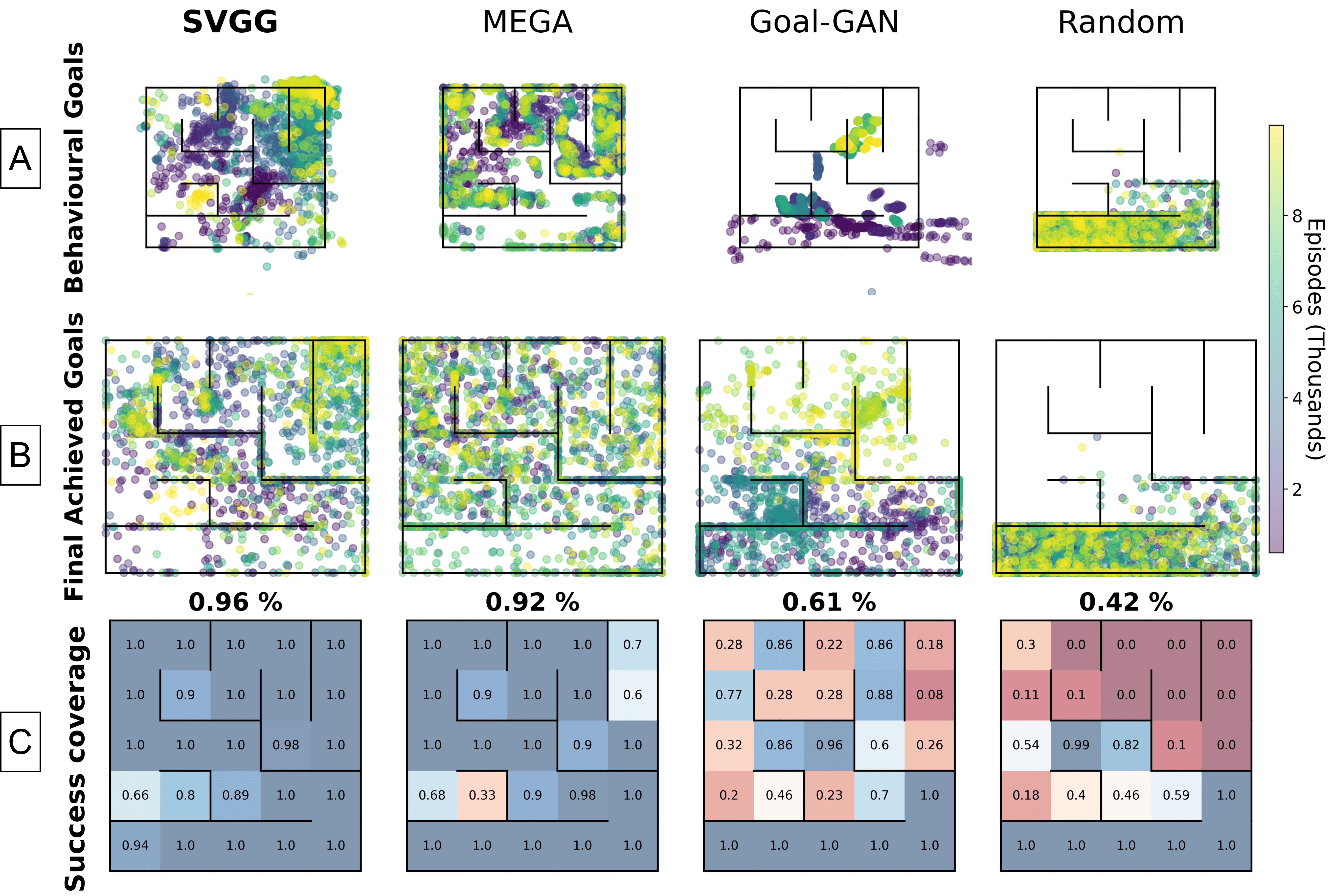
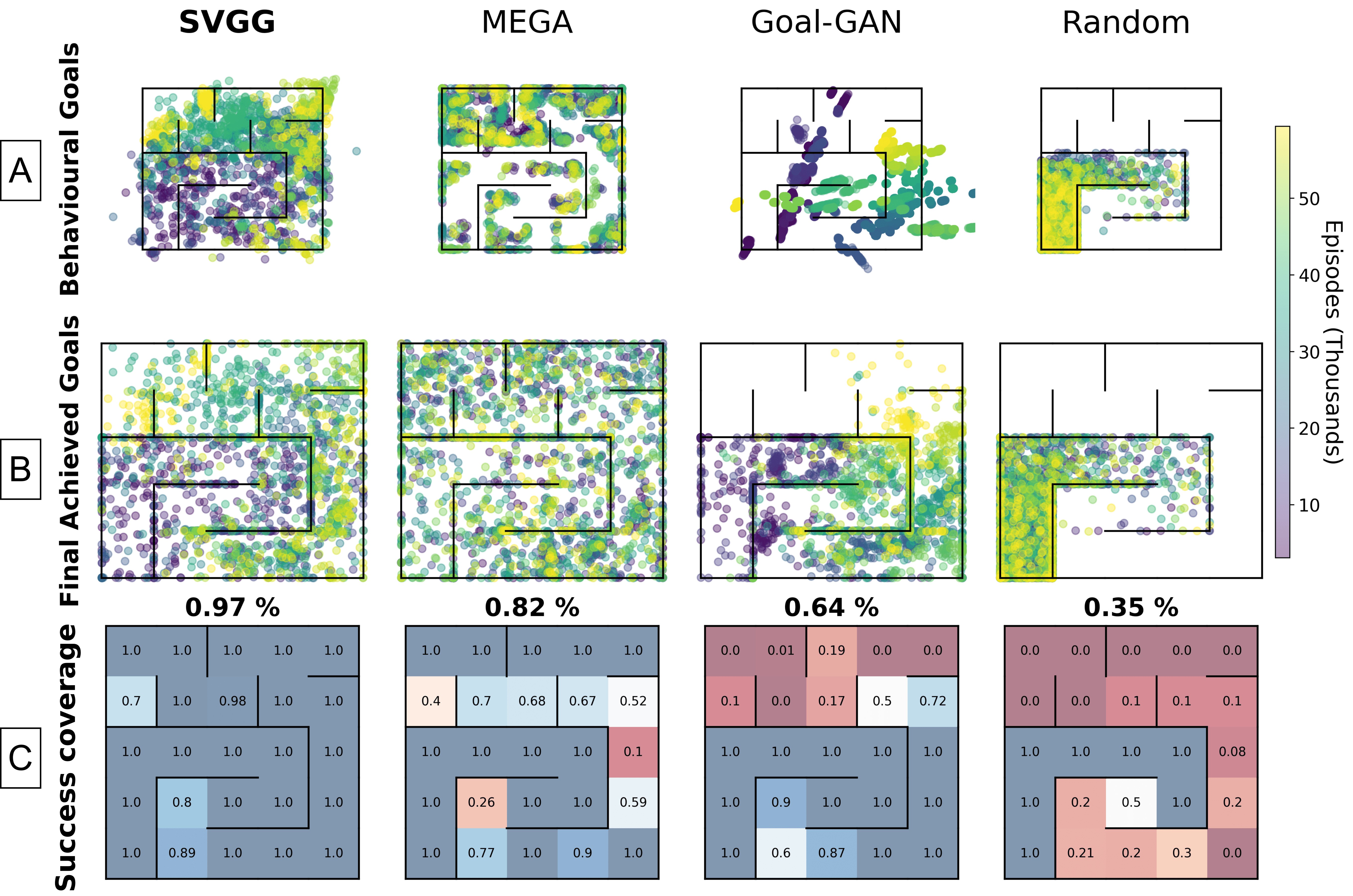
We visualize behavioral and achieved goals in Maze 1 (Figure 5) and Maze 2 (Figure 6), in parallel with the success coverage after training. The main advantages of our method lie in the capacity to target difficult areas and avoid catastrophic forgetting, which results in nearly optimal success coverage. We observe that mega efficiently discovers the environment but fails to master the corresponding goals. This also leads to catastrophic forgetting and a lack of adaptation when the environment changes, as studied in the main paper.
One can see that the generation of GOIDs in Goal gan is very unstable and tricky in such discontinuous goal space, especially as the generator is susceptible to output goals outside the environment boundary, which svgg avoids with the validity distribution.
Appendix C Additional experiments details
C.1 Environments
Pointmaze
We use a 2D pointmaze environment where the state space and goal space are (x, y) coordinates (the agent cannot see the walls), and the agent moves according to its action, which is a 2-dimensional vector with dimensions constrained to . All methods are tested on four mazes with different shapes and a highly discontinuous goal space. The maximum number of steps in one trajectory is set to 30. We argue that the difficulty of these environments does not lie in their size, but rather in the complexity of their goal space and thus of the trajectories adopted by the agent to achieve these goals.
Antmaze
An Ant has to move around in a U-shape hallway maze of size 20x4, the goal space remains coordinates of the Ant as in Pointmaze. However, the exploratory behavior is much simpler than in the considered pointmazes environments, as the maze is simply U-shaped. The difficulty lies in the control of the Ant dynamics, as it must move its legs with a 8-dimensional action space and the observation space is a 30-dimensional vector corresponding to the angles of the legs.
FetchPickAndPlace (Hard version)
We also perform comparisons on a hard version of FetchPickAndPlace-v1 from OpenAI gym (Brockman et al., 2016). The agent controls a robotic arm which must pick and place a block to a 3D desired location. In the hard version, the behavioral goals are all between 20 and 45cm in the air, while in the original version, 50% of behavioral goals are on the table and the remaining ones are from 0 to 45cm in the air.
While this environment presents a greater difficulty in terms of control (the action dimension is 4 and the state dimension is which correspond to the various positions of the robot joint), the goal generation component is significantly easier: as the 3-dimensional goal space is smooth, there is no obstacle for the agent to bypass. As Figure 2 shows, svgg solves the environment within 1.5M steps, but does not significantly outperform mega.
We argue that the interest of our goal generation algorithm resides in environments with highly discontinuous goal space as the action control is largely supported by the RL algorithm (e.g. ddpg). Therefore, the smaller difference between mega and svgg in this environment was expected, as svgg is mainly designed to target non-smooth goal spaces, and to avoid pitfalls such as catastrophic forgetting.
FetchReach (Stuck version)
We compare svgg to baselines with a modified version of the FetchReach environment, where the gripper is initially stuck between four walls and has to carefully navigate between them to reach the goals. The observations are 9-dimensional vectors, the actions as well as the goals are 3-dimensional. The success coverage is computed on uniformly sampled goals with a target range fixed to , which corresponds to the maximal L2 distance between the goal and the initial gripper position. The initial task is solved within steps by all baselines, whereas with the modified version, only svgg achieves a success rate in 3M steps.
FetchPush (Maze version)
We add a maze structure with walls on the table to the FetchPush benchmark to once again add discontinuities in the goal space. The observations are 24-dimensional vectors, the actions as well as the goals are 3-dimensional. The success coverage is computed on goals uniformly sampled on the table, and the block’s initial position is sampled behind the first wall on the robot side. The standard FetchPush task was solved by svgg and mega in less than 1M steps. The maze version is much harder: svgg achieves a success coverage rate within 10M steps, whereas mega barely reaches . The distance to reach the goals in all environments is .
Appendix D Control of the sampling difficulty
Using beta distributions makes it possible to tune the goal difficulty an agent should aim at to efficiently explore and control an environment. Indeed, by tuning the and hyper-parameters of the distribution, one gets a different incentive for goal difficulty. We choose to compare the efficiency of 5 pairs of and hyper-parameters, as illustrated in Figure 7.
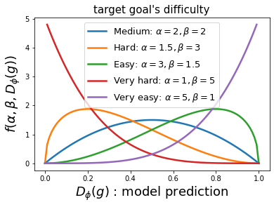
In Figure 8, we compare the 5 versions of svgg using different beta distributions from Figure 7, on the 4 previously considered mazes. One can observe that extreme targets difficulties are the least effective ones, especially the Very easy, which is too conservative to efficiently explore new areas of the space. On the other hand, svgg performs very well with Medium and Hard distributions. This suggests that the optimal goal difficulty is somewhere between medium and hard. Performing a more advanced optimization over and is left for future work.

Appendix E Target goal distribution ablations
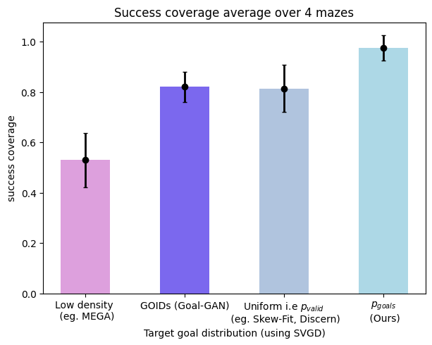
We conduct an ablation which consists in keeping svgd, but replacing our target goal distribution (corresponding to goals whose prediction of success is close to 0.5) with the target goal distributions of related work such as of Skew-Fit, mega or Goal gan (resp. the uniform distribution over the support of achieved goals, the region of low density of achieved goals and goals of intermediate difficulty (GOIDs)). For all criteria, the goal target distribution is represented as a set of particles and optimized with svgd. We compare the average success coverage over our 4 mazes on Figure 9 where we can see that our choice of target distribution is the most effective. We describe below the compared goals’ distribution.
Uniform distribution over the support of achieved goals (as in Skew-Fit and discern):
This corresponds to our "Only validity" baseline in Figure 2. Indeed, the probability for a goal to be valid is learned with a One Class SVM which exactly strives to uniformly cover the distribution of achieved goals. As the results presented in Figure 9 show, this baseline performs relatively well, but is unable to target areas where the agent struggles. Therefore, it is not as efficient as our target distribution .
Distribution derived from the region of low density of achieved goals (as in mega):
We can obtain a distribution of goals very close to mega ’s by combining our “Only Validity” ablation with a beta distribution tuned to address the lowest probability region (i.e taking ), with a Beta distribution and and set to target low density of ). Due to the absence of a mechanism to avoid sampling unfeasible goals, the particles are attracted to low density areas that mostly correspond to non-valid goals, which make this baseline very inefficient.
distribution of GOIDs (as in Goal gan):
Our target distribution is very close to the GOID in Goal gan, the main difference is the smoothness of our Beta distribution versus the indicator function of Goal gan that labels a goal as of "intermediate difficulty" when the probability of reaching it in an interval (eg. between 0.2 and 0.8). So, to move closer to the Goal gan criterion, we replaced the beta-distribution used in svgg with the crisp distribution (with a generalized Gaussian distribution of skewing parameter ) which outputs 1 for probabilities between 0.3 and 0.7 and 0 otherwise (which are the parameters that give the best results). Note that while this distribution is differentiable, the gradient is less informative than our version. As a consequence, approximating this distribution with svgd is less efficient and gets a lower success coverage.
Appendix F Sampling method ablations
To highlight the interest of the svgd choice to sample goals from our target distribution , we conducted additional experiment where we swap svgd with some other sampling tools : MCMC (Metropolis Hastings), GANs and direct sampling from the replay buffer.
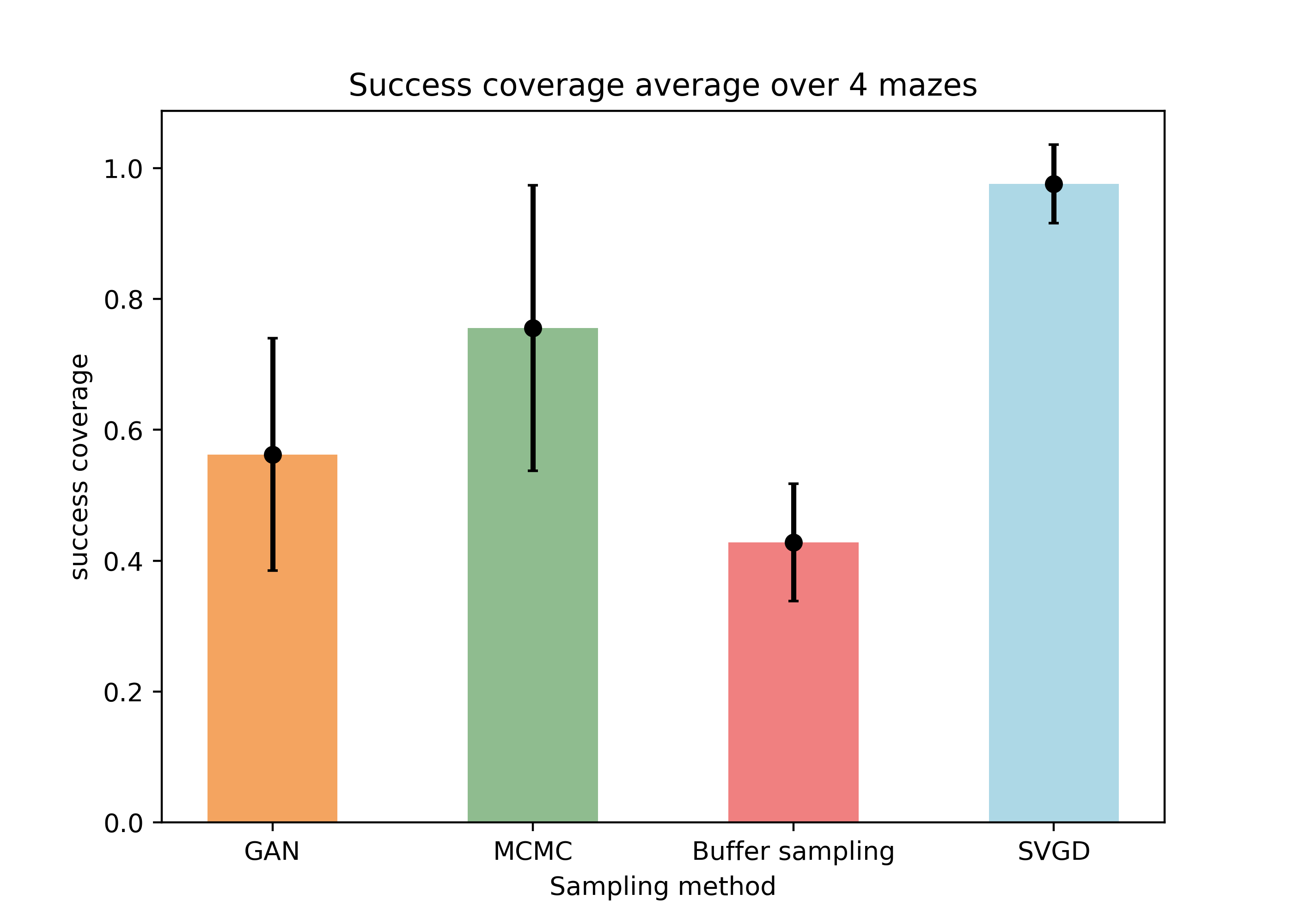
In Figure 10 we can see that svgd is by far the most efficient way to sample from and thus maximize the success coverage. We describe below the tested sampling tools.
GANs
: We use the same procedure as Goal gan by replacing their criterion by our target distribution . the results are very similar to Goal gan, this can be explained by the proximity of our criterion in terms of intermediate difficulty, except from the fact that we add , we can also conclude that GANs are not the best choice for moving target distributions due to their training instability. We use the same hyperparameters as in the Goal gan baseline.
Buffer sampling
: We sample a batch of previously achieved goals in the buffer, and then compute a categorical distribution based on the criterion and sample candidate goals. This method is the least effective baseline, which was expected as the exploration component was provided by svgd, the goals from the replay buffer are not sufficiently diverse to explore the environment if not combined with a diversity criterion.
MCMC (Metropolis Hastings)
: At each update, we construct a markov-chain with normal movement (with and ) then classic likelihood ratio rejection sampling to draw goals samples that are provided to the agent. Metropolis-Hastings is a good candidate but is still far from the svgd performance, it presents some good sampling accuracy at times but is very slow to converge to the true distribution, thus the goal sampling isn’t always aligned with the agent skills at the time, and enable the recovery property.
Appendix G Methods details
We first focus on the behavioral goal sampling strategy. We use ddpg with her to learn how to reach a goal in svgg, mega and Goal gan. ddpg is parameterized as in Table 1. All algorithms are run using the same number of training epochs .
| DDPG Hyper-Parameters | Value |
| Batch size for replay buffer | 2000 |
| Discount factor | 0.99 |
| Action L2 regularization | 0.1 |
| (Gaussian) Action noise max std | 0.1 |
| Warm up steps before training | 2500 |
| Actor learning rate | 1e-3 |
| Critic learning rate | 1e-3 |
| Target network soft update rate | 0.05 |
| Actor & critic networks activation | Gelu |
| Actor & critic hidden layers sizes | |
| Replay buffer size | nb training steps |
G.1 Hindsight Experience Replay
The original goal relabeling strategy introduced in her (Andrychowicz et al., 2017) is the future, which consists in relabeling a given transition with a goal achieved on the trajectory later on. This is very effective in sparse reward setting to learn a GCP. However, many works suggested that relabeling transitions with goals outside the current trajectory helps the agent generalize across trajectories. For example, one can use inverse RL to determine the optimal goal to relabel a given transition (Eysenbach et al., 2020). We use a naive version of this method. As in (Pitis et al., 2020), we relabel transitions for ddpg optimization using a mixed strategy. All methods presented in this work use the same strategy.
10% of real experience are kept while 40% of the transitions are relabeled using the future strategy of her. We relabel the remaining 50% transitions with goals outside of their trajectory, with randomly sampled goals among the past behavioral and achieved goals. The latter part of the strategy helps share information between different trajectories that often contains similar transitions.
G.2 SVGG
svgg is described in the main paper, in this section, we go through implementation details and hyper-parameters.
| SVGG Hyper-Parameters | Symbol | Value |
| SVGD | ||
| Number of particles | 100 | |
| Optimization interval (in steps) | 20 | |
| Nb of particle moves per optim. | 1 | |
| RBF kernel bandwidth | 1 | |
| Learning rate | 1e-3 | |
| Agent’s skill model | ||
| Hidden layers sizes | (64, 64) | |
| Gradient steps per optimization | 10 | |
| Learning rate | 1e-3 | |
| Training batch size | 100 | |
| Training history length (episodes) | 1000 | |
| Optimization interval (in steps) | 4000 | |
| Nb of training steps | 100 | |
| Activations | Gelu | |
| OCSVM validity distribution | ||
| RBF kernel bandwidth | 1 | |
| Optimization interval (in steps) | 4000 |
G.3 MEGA
The authors of mega (Pitis et al., 2020) train a GCP with previously achieved goals from a replay buffer. Their choice of goals relies on a minimum density heuristic, where they model the distribution of achieved goals with a KDE. They argue that aiming at novel goals suffices to efficiently discover and control the environment. We use the original implementation of the authors, the pseudocode is given in Algorithm 3 and specific hyper-parameters are in Table 2.
| MEGA Hyper-parameters | Symbol | Value |
| RBF kernel bandwidth | 0.1 | |
| KDE optimization interval (in steps) | 1 | |
| Nb of state samples for KDE optim. | 10.000 | |
| Nb of sampled candidate goals | 100 | |
| -value cutoff | -3 |
G.4 GoalGAN
Goal gan (Florensa et al., 2018) uses a procedural goal generation method based on GAN training. As our svgg, it aims at sampling goals of intermediate difficulty, which they define as , being the probability for the policy to achieve goal , and are hyper-parameters. A Discriminator is trained to distinguish between goals in and other goals, while a generator is trained to output goals in by relying on the discriminator outputs. They optimize and in a manner similar to the Least-Squares GAN (LSGAN) with the following losses:
| (7) |
where is the label that indicates whether belongs to or not. In (Florensa et al., 2018), the authors use Monte-Carlo sampling of the policy to estimate . For efficiency reasons, we use a learned model of the agent’s capabilities as in svgg. The pseudocode is given in Algorithm 4 and specific hyper-parameters are in Table 3.
| GoalGAN Hyper-parameters | Symbol | Value |
| Gaussian prior dimension | 4 | |
| Generator hidden layers sizes | (64, 64) | |
| Discriminator hidden layers sizes | (64, 64) | |
| Optimization interval (in steps) | 2000 | |
| GAN training batch size | 200 | |
| Nb of GAN optimization steps | 100 | |
| GAN Learning rate | 1e-3 | |
| Minimum GOID probability | 0.1 | |
| Maximum GOID probability | 0.9 |
G.5 Ressources
Every seed of each experiment was run on 1 GPU in the following list {Nvidia RTX A6000, Nvidia RTX A5000, Nvidia TITAN RTX, Nvidia Titan Xp, Nvidia TITAN V}. The total training time is close to 4.000 hours, most of it executed in parallel, as we had full time access to 12 GPUs.