FISAR: Forward Invariant Safe Reinforcement Learning
with a Deep Neural Network-Based Optimizer
Abstract
This paper investigates reinforcement learning with constraints, which are indispensable in safety-critical environments. To drive the constraint violation to decrease monotonically, we take the constraints as Lyapunov functions and impose new linear constraints on the policy parameters’ updating dynamics. As a result, the original safety set can be forward-invariant. However, because the new guaranteed-feasible constraints are imposed on the updating dynamics instead of the original policy parameters, classic optimization algorithms are no longer applicable. To address this, we propose to learn a generic deep neural network (DNN)-based optimizer to optimize the objective while satisfying the linear constraints. The constraint-satisfaction is achieved via projection onto a polytope formulated by multiple linear inequality constraints, which can be solved analytically with our newly designed metric. To the best of our knowledge, this is the first DNN-based optimizer for constrained optimization with the forward invariance guarantee. We show that our optimizer trains a policy to decrease the constraint violation and maximize the cumulative reward monotonically. Results on numerical constrained optimization and obstacle-avoidance navigation validate the theoretical findings.
I Introduction
Reinforcement learning (RL) has achieved remarkable success in robotics [1, 2, 3]. In general, an RL agent is free to explore the entire state-action space and improves its performance via trial and error [4]. However, there are many safety-critical scenarios where an agent cannot explore certain regions. For example, a self-driving vehicle must stay on the road and avoid collisions with other cars and pedestrians. An industrial robot also should not damage the safety of the workers. Another example is a medical robot, which should not endanger a patient’s safety. Therefore, an effective agent should satisfy certain safety constraints during its exploration, and failure to do so can result in undesirable outcomes.
The safe exploration problem can be represented by the constrained Markov decision process (CMDP) [5]. Existing optimization techniques to solve CMDP include the vanilla Lagrangian method [6], which solves a minimax problem by alternating between primal policy and dual variables. Further, a PID Lagrangian method in [7] addresses the oscillations and overshoot in learning dynamics that lead to constraint violation. However, these methods show difficulties when solving a minimax problem with non-convexity (e.g., non-linear function approximations). Another approach solves CMDP as non-convex optimization directly via successive convexification of the objective and constraints [8, 9]. However, the convexification methods also have several drawbacks: 1) there is a lack of understanding of how the constraint is driven to be feasible (e.g., at what rate does the constraint violation converge to zero?), 2) the convexified subproblem can often encounter infeasibility, requiring a heuristic to recover from infeasibility, and 3) it needs to solve convex programming with linear/quadratic objective and quadratic constraints at every iteration, which is inefficient.
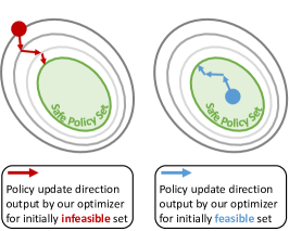
In this paper, we introduce a new learning-based framework to address the aforementioned limitations in solving CDMP. Specifically, we propose to take safety constraints as Lyapunov functions to drive the constraint violation monotonically decrease and impose new constraints on the updating policy dynamics. We note that such new constraints, which are linear inequalities and guaranteed to be feasible, can guarantee the forward invariance: the constraint violation can converge asymptotically if the policy initialization is infeasible, and the trajectory will stay inside the feasible set if the policy initially starts there (see Figure 1). However, with the new constraints imposed on the policy update dynamics, it is difficult to design such updating rules to optimize the objective while simultaneously satisfying the constraints. Methods like projected gradient descent [10] are not applicable here because the constraints are on the updating dynamics instead of on the primal variables. Therefore, we propose to learn an optimizer parameterized by a deep neural network, where the constraint-satisfaction is guaranteed by projecting the optimizer output onto those linear inequality constraints. While generic projection onto polytopes formulated by multiple linear inequalities cannot be solved in closed form, we design a proper metric for the projection such that it can be solved analytically.
Contribution. In summary, our contributions are twofold. First, We propose a model-free framework to learn a deep neural network-based optimizer to solve a safe RL problem formulated as a CMDP with guaranteed feasibility without solving a constrained optimization problem iteratively, unlike the algorithms based on successive convexification [8, 9]. To the best of our knowledge, this is the first generic DNN-based optimizer for constrained optimization and can be applied beyond the safe learning context. Second, the resulting updating dynamic of the policy parameters implies forward-invariance of the safety set. Hence, our method theoretically guarantees that the constraint violation will converge asymptotically, which has not been established yet among existing safe reinforcement learning works.
II Related Works
Safe reinforcement learning. Algorithms from a control-theoretic perspective mainly fall into the category of Lyapunov methods. For tabular settings, Lyapunov functions are constructed in [11] to guarantee global safety during training via a set of local linear constraints. Another work obtains high-performance control policies with provable stability certificates using the Lyapunov stability verification [12]. Recently, [13] constructs a neural network Lyapunov function and trains the network to the shape of the largest safe region in the state space.
On the other hand, the control barrier function [14] provides a venue to calibrate the potentially unsafe control input to the safety set. For example, [15] introduces an end-to-end trainable safe RL method, which compensates the control input from the model-free RL via model-based control barrier function. To avoid solving an optimization problem while guaranteeing safety, the vertex network [16] formulates a polytope safety set as a convex combination of its vertices. In [17], an input-output linearization controller is generated via a control barrier function and control Lyapunov function based quadratic program with the model uncertainty learned by reinforcement learning.
There are also approaches to solve a safe RL problem with temporal logic specifications [18, 19] and curriculum learning [20]. See [21] for in-depth surveys about safe RL.
Compared to these approaches, our method is based on the model-free policy gradient reinforcement learning, so neither the transition dynamics nor the cost function is explicitly needed. Additionally, our approach guarantees forward invariance, so the policy will be updated to be only safer.
DNN-based optimizer. In contrast to hand-designed optimization algorithms, [22] proposes to cast the design of a gradient-based optimization algorithm as a learning algorithm. This work is then further extended to learn a gradient-free optimizer in [23]. Recently, [24] introduces the Meta-SGD, which can initialize and adapt to any differentiable learner in just one step. This approach shows a highly competitive performance for few-shot learning settings. To improve the scalability and generalization of DNN-based optimizers, [25] develops a hierarchical recurrent neural network architecture that uses a learned gradient descent optimizer. For more information about deep neural network-based optimizers, we refer to the survey [26]. However, these previous works are designed for unconstrained optimization. In this paper, we extend these approaches and develop a DNN-based optimizer for constrained optimization.
III Preliminary
III-A Markov decision process
The Markov decision process (MDP) is a tuple , where is the set of the agent state in the environment, is the set of agent actions, is the transition function, denotes the reward function, is the discount factor and is the initial state distribution. A policy is a mapping from the state space to probability over actions. denotes the probability of taking action under state following a policy parameterized by . The objective is to maximize the cumulative reward:
| (1) |
where and are trajectories sampled under . To optimize the policy that maximizes (1), the policy gradient with respect to can be computed as [27]: where [4].
III-B Constrained Markov decision process
The constrained Markov decision process (CMDP) is defined as a tuple , where is the cost function and the other variables are identical to those in the MDP definition (see Section III-A) [5]. The goal in CMDP is to maximize the cumulative reward while satisfying the constraints on the cumulative cost:
| (2) | |||
where is the policy parameters, , is the constraint set, and is the maximum acceptable violation of . In a later context, we use and as short-hand versions of and , respectively, for clarity. While the discount factor for the cost can be different from that for the reward, we use the same for notational simplicity.
Instead of imposing safety constraints on the cumulative cost (see (2)), there is another option of imposing them on individual state-action pairs [15, 16]:
| (3) | |||
where and denotes the horizon of the MDP. We note that (2), the problem formulation considered in this work, is more general than (3) in two aspects. First, the constraint on each individual state-action pair can be transformed into the form of cumulative cost via setting binary cost function followed by summation with in a finite horizon MDP. That is to say, the constraints in (3) can be re-written equivalently in the form of the constraints in (2) as , where is an indicator function such that if and otherwise. Second, in scenarios where the agent can afford a certain amount of violations (i.e., in (2)) throughout an episode, it is infeasible to allocate it to individual time instances. An example scenario is a video game, where a player can stand some given amount of attacks in the lifespan before losing the game.
III-C Control barrier functions
Consider the following non-linear control-affine system:
| (4) |
where and are locally Lipschitz, is the state and is the set of admissible inputs. The safety set is defined as with . Then is a control barrier function (CBF) [14] if there exists an extended class- function such that for the control system (4):
| (5) |
where is the Lie derivative.
IV Approach
IV-A Forward-invariant constraints on updating dynamics
The key to solving (2) is how to deal with the constraints. Existing methods [6, 8] often encounter oscillations and overshoot [7] in learning dynamics that can result in noisy constraint violations. In this paper, we aim to address this issue and build a new mechanism that drives the constraint violation to converge asymptotically if the initialization is infeasible. Otherwise, the trajectory will stay inside the feasible set (i.e., forward invariance). To accomplish our goal, we start by building a Lyapunov-like condition:
| (6) |
where is the updating dynamics of and is an extended class- function. Note that such Lyapunov functions are directly taken from the constraint functions so that this process needs no extra effort. A special case of the class- function is a scalar linear function with positive slope and zero intercept. With discretization, the updating rule becomes:
| (7) |
where denotes the learning rate. Note that, with sufficiently small , the continuous dynamics can be approximated with a given accuracy. 1 characterize how (6) will make the safety set forward invariant. For notational simplicity, the statement is on one constraint with and . This simplification does not lose any generality because the joint forward-invariance of multiple sets will naturally lead to the forward-invariance of their intersection set.
Lemma 1
Consider a continuously differentiable set with defined on . Then is forward invariant, if is a superset of (i.e., ), and (6) is satisfied.
Proof: Define as the boundary of . As a result, for , . Then, according to the Nagumo’s theorem [28, 29], the set is forward invariant.
Here we provide intuition behind (6). Using the chain rule: . Then, the solution to this partial differential equation is . With , it means that the initialization is infeasible (i.e., ), and thus will converge to (i.e., the boundary of ) asymptotically. It is similar with a feasible initialization (i.e., ). It is worth noting that with , i.e., the number of constraints is smaller than that of the policy parameters, (6) is guaranteed to be feasible. This saves the trouble of recovering from infeasibility in a heuristic manner, which is usually the case for the previous approaches [8, 9].
While (6) in our proposed method looks similar to (5) in CBF, our method is substantially different from those exploiting CBF [15, 16]. First, CBF-based methods require the system dynamics in (4) while our method is model-free, not requiring transition dynamics and cost function in (2) (in parallel to in (5)). Second, it is more significant that (5) and (6) represent different meanings. On one hand, the former represents the constraint on the control input , given a state at a certain time instance , while in the latter, is evaluated on multiple time instances (e.g., one episode). Due to this, considering multiple time instances can help make a globally optimal decision while one-step compensation can be short-sighted. On the other hand, if we further replace by , a policy parameterized by , (5) becomes a non-linear constraint on policy parameter at time instance , while (6) is a constraint imposed on instead of . Such constraint on the updating dynamics can result in forward invariance directly in the policy space ( therein). By contrast, the forward-invariance of CBF is in the state space ( therein), and thus it still requires to solve an optimization problem to generate a control input [15] at each time instance, which can be computationally inefficient.
IV-B Learning a deep neural network-based optimizer
So far, we have converted the constraint on in (2) to that on in (6), which formulates the new set
| (8) |
and . However, it is unclear how to design an optimization algorithm that minimizes the objective in (2) while satisfying (6). Note that the typical constrained optimization algorithms, such as projected gradient descent (PGD), are no longer applicable because the constraints are not on the primal variables anymore. Specifically, similar to the PGD mechanism, can be updated in the following way:
| (9) |
where is the projection operator onto the set . However, this can be problematic as it is ambiguous whether is still an ascent direction. Consequently, standard optimization algorithms (e.g., stochastic gradient descent (SGD), ADAM [30]) with (9), will fail to optimize the objective while satisfying the constraints as we will show in the result section. Thus, we propose to learn a DNN-based optimizer.
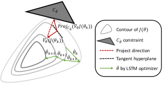
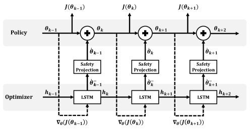
Following the work by [22], which learns an optimizer for unconstrained optimization problems, we extend it to the domain of constraint optimization. Our optimizer is parameterized by a long short-term memory (LSTM, [31]) with as the parameters for the LSTM network . We note that the recurrence nature of LSTM allows to learn dynamic update rules by fully exploiting historical gradient information, similar to the momentum-based optimization techniques [32, 30]. Similar to [22], the updating rule becomes:
| (10) | |||
where is the hidden state for . The loss to train the optimizer parameter is defined as:
| (11) |
where is the span of the LSTM sequence and is the weight coefficient. Given this loss function, aims to generate the updating direction of in the whole horizon such that the final is optimal. The main difference between ours and [22] is the projection step (i.e., the second line in (IV-B)). As a result, it can be understood that the end-to-end training minimizes the loss in (11) while the constraint-satisfaction is guaranteed by the projection.
Here we take a further qualitative analysis on the difference between the updating rules in (9) and (IV-B) and validate the advantage of the latter. During the iterations of maximizing , one-step projected gradient can result in a descent direction (i.e., the other side of the tangent hyperplane in Figure 2) and is difficult to guarantee performance through the iterations. By contrast, , output from the LSTM optimizer, will take the whole optimization trajectory into consideration (see the loss function (11)) to eventually maximize , the objective function value at the last step, even some intermediate steps can have a few objective descents as well (e.g., in Figure 2).
IV-C Solving projection onto general polytope analytically
Even is a polytope formulated by linear inequalities, projection onto is still non-trivial and requires an iterative solver such as in [8], except that there is only one inequality constraint (i.e., ). Two alternative methods are proposed in [33]: one is to find the single active constraint to transform into a single-constraint case and the other is to take the constraints as a penalty. However, the former is troublesome and possibly inefficient and the latter will sacrifice the strict satisfaction of the constraint.
Hence, we propose to solve the projection onto the polytope formulated by multiple linear inequalities in a closed form. We first explain the generic projection problem onto a polytope:
| (12) |
where , is of full row rank and is positive definite. Then the dual problem of (IV-C) is
| (13) |
The dual problem in (13) generally cannot be solved analytically as is positive definite but not diagonal. Though is usually set as the identity matrix, it is not necessary other than that should be positive definite. As a result, we design such that is diagonal by solving:
| (14) | |||||
where . As a result, we obtain . Then (13) can be solved in closed form as:
| (15) |
The schematics of the LSTM-based optimizer is presented in Figure 3 and the algorithm FISAR (Forward Invariant SAfe Reinforcement learning) is summarized in algorithm 1.
V Experiments
As our LSTM-parameterized optimizer applies to general constrained optimization problems, it is first tested on a non-linear numerical optimization problem. Then, we evaluate our safe RL framework in an obstacle-avoidance navigation environment.
V-A Quadratically constrained quadratic programming
We first apply the learned LSTM-optimizer on the following quadratically constrained quadratic programming (QCQP), which has various applications including signal processing [34], graph theory [35], and optimal control [36]. Specifically, the objective and constraints in this domain are defined as:
| (16) |
where , and . here is not necessarily positive semi-definite and thus can bring non-convexity.
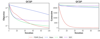
We solve QCQP using our LSTM-optimizer as well as three unconstrained baselines (Adam, RMS, and SGD) to show the scale of the objective. Given the results in Figure 4, in this deterministic setting, the constraint violation is driven to satisfaction asymptotically, while our objective is comparable to that from the unconstrained solvers.
V-B Obstacle-avoidance navigation
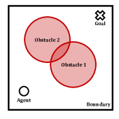
We build a domain where a particle agent tries to navigate in 2D space with obstacles to reach the goal position (see illustration in Figure 5). The system uses double-integrator dynamics. The reward function is set as , where is the coordination of the particle and . For obstacle , , the associated cost function is defined as if and otherwise, where is the center of .
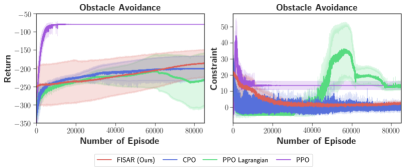
We use the policy gradient reinforcement learning algorithm to solve this problem, where the policy is parameterized by deep neural networks and trained by our LSTM-optimizer. We compare our algorithm against two state-of-the-art safe RL baselines, the Lagrangian [6] and constrained policy optimization (CPO) [8] method. We use an open-source implementation for these baselines111https://github.com/openai/safety-starter-agents. For a reference, we also compare against an unconstrained RL algorithm, proximal policy optimization (PPO), using an open-source implementation222https://spinningup.openai.com/. For reproducibility, the hyperparameters of all the implemented algorithms can be found in the appendix.
Results of the policy trained by our optimizer and the baselines are demonstrated in Figure 6. There are two notable observations. First, as expected, the unconstrained baseline of PPO achieves the highest return while showing the large constraint violation. Second, FISAR drives the constraint function to decrease to satisfaction almost monotonically, but CPO’s constraint function is much nosier and PPO-Lagrangian eventually cannot satisfy the constraints. FISAR achieves the smoother constraint satisfaction with a similar return compared to CPO and PPO Lagrangian baseline.
The failure of the PPO-Lagrangian method may come from the difficulty of solving a minimax problem such that the algorithm gets stuck into a local minimax point, where the primal constraints are not satisfied yet. For the CPO, the successive convexification can be the reason for the oscillation of the constraints within the trust region. However, if the trust region is tuned smaller, the learning process will be slower, resulting in higher sample complexity.
VI Conclusion
In this paper, we propose to learn a DNN-based optimizer to solve a safe RL problem formulated as CMDP with guaranteed feasibility without solving a constrained optimization problem iteratively. Moreover, the resulting updating dynamics of the variables imply forward-invariance of the safety set. Future work will focus on applying the proposed algorithm in more challenging RL domains as well as more general RL algorithms such as actor-critic and extending it to multiagent RL domains with non-stationarity. The challenge for the latter can partly come from that the safety constraints can be coupled among multiple agents (e.g., collision avoidance), which makes it difficult to get a decentralized policy for each agent.
Acknowledgements
Dong-Ki Kim was supported by IBM, Samsung (as part of the MIT-IBM Watson AI Lab initiative), and Kwanjeong Educational Foundation Fellowship. We thank Amazon Web services for computational support.
The hyperparameters for our method and the baselines can be found in the following table, where “NN” and “lr” stand for “neural network” and “learning rate”, respectively. For other parameters, we use the default ones in the repositories.
| General | |||
|---|---|---|---|
| Parameter | Value | Parameter | Value |
| Policy NN type | MLP | Policy lr | 0.001 |
| Policy NN hidden size | 16 | 0.99 | |
| Episode length | 100 | ||
| FISAR (Ours) | |||
| Parameter | Value | Parameter | Value |
| LSTM hidden number | 128 | in (11) | 120 |
| LSTM hidden layer | 2 | batch size | 24 |
| LSTM training lr | 0.05 | in (6) | 20 |
| in (IV-B) | 0.001 | ||
| CPO, PPO-Lagrangian, PPO | |||
| Parameter | Value | ||
| (GAE) | 0.95 |
References
- [1] J. Schulman, P. Moritz, S. Levine, M. Jordan, and P. Abbeel, “High-dimensional continuous control using generalized advantage estimation,” in Proceedings of the International Conference on Learning Representations (ICLR), 2016.
- [2] S. Levine, C. Finn, T. Darrell, and P. Abbeel, “End-to-end training of deep visuomotor policies,” J. Mach. Learn. Res., vol. 17, no. 1, p. 1334–1373, Jan. 2016.
- [3] S. Gu, E. Holly, T. Lillicrap, and S. Levine, “Deep reinforcement learning for robotic manipulation with asynchronous off-policy updates,” in 2017 IEEE International Conference on Robotics and Automation (ICRA), 2017, pp. 3389–3396.
- [4] R. S. Sutton and A. G. Barto, Reinforcement learning: An introduction. MIT press, 2018.
- [5] E. Altman, Constrained Markov decision processes. CRC Press, 1999, vol. 7.
- [6] Y. Chow, M. Ghavamzadeh, L. Janson, and M. Pavone, “Risk-constrained reinforcement learning with percentile risk criteria,” The Journal of Machine Learning Research, vol. 18, no. 1, pp. 6070–6120, 2017.
- [7] A. Stooke, J. Achiam, and P. Abbeel, “Responsive safety in reinforcement learning by pid lagrangian methods,” arXiv preprint arXiv:2007.03964, 2020.
- [8] J. Achiam, D. Held, A. Tamar, and P. Abbeel, “Constrained policy optimization,” in Proceedings of the 34th International Conference on Machine Learning-Volume 70. JMLR. org, 2017, pp. 22–31.
- [9] M. Yu, Z. Yang, M. Kolar, and Z. Wang, “Convergent policy optimization for safe reinforcement learning,” in Advances in Neural Information Processing Systems, 2019, pp. 3121–3133.
- [10] Y. Nesterov, Introductory lectures on convex optimization: A basic course. Springer Science & Business Media, 2013, vol. 87.
- [11] Y. Chow, O. Nachum, E. Duenez-Guzman, and M. Ghavamzadeh, “A lyapunov-based approach to safe reinforcement learning,” in Advances in neural information processing systems, 2018, pp. 8092–8101.
- [12] F. Berkenkamp, M. Turchetta, A. Schoellig, and A. Krause, “Safe model-based reinforcement learning with stability guarantees,” in Advances in neural information processing systems, 2017, pp. 908–918.
- [13] S. M. Richards, F. Berkenkamp, and A. Krause, “The lyapunov neural network: Adaptive stability certification for safe learning of dynamical systems,” arXiv preprint arXiv:1808.00924, 2018.
- [14] A. D. Ames, X. Xu, J. W. Grizzle, and P. Tabuada, “Control barrier function based quadratic programs for safety critical systems,” IEEE Transactions on Automatic Control, vol. 62, no. 8, pp. 3861–3876, 2016.
- [15] R. Cheng, G. Orosz, R. M. Murray, and J. W. Burdick, “End-to-end safe reinforcement learning through barrier functions for safety-critical continuous control tasks,” in Proceedings of the AAAI Conference on Artificial Intelligence, vol. 33, 2019, pp. 3387–3395.
- [16] L. Zheng, Y. Shi, L. J. Ratliff, and B. Zhang, “Safe reinforcement learning of control-affine systems with vertex networks,” arXiv preprint arXiv:2003.09488, 2020.
- [17] J. Choi, F. Castañeda, C. J. Tomlin, and K. Sreenath, “Reinforcement learning for safety-critical control under model uncertainty, using control lyapunov functions and control barrier functions,” arXiv preprint arXiv:2004.07584, 2020.
- [18] M. Alshiekh, R. Bloem, R. Ehlers, B. Könighofer, S. Niekum, and U. Topcu, “Safe reinforcement learning via shielding,” arXiv preprint arXiv:1708.08611, 2017.
- [19] N. Fulton and A. Platzer, “Safe reinforcement learning via formal methods,” in AAAI Conference on Artificial Intelligence, 2018.
- [20] M. Turchetta, A. Kolobov, S. Shah, A. Krause, and A. Agarwal, “Safe reinforcement learning via curriculum induction,” arXiv preprint arXiv:2006.12136, 2020.
- [21] J. Garcıa and F. Fernández, “A comprehensive survey on safe reinforcement learning,” Journal of Machine Learning Research, vol. 16, no. 1, pp. 1437–1480, 2015.
- [22] M. Andrychowicz, M. Denil, S. Gomez, M. W. Hoffman, D. Pfau, T. Schaul, B. Shillingford, and N. De Freitas, “Learning to learn by gradient descent by gradient descent,” in Advances in neural information processing systems, 2016, pp. 3981–3989.
- [23] Y. Chen, M. W. Hoffman, S. G. Colmenarejo, M. Denil, T. P. Lillicrap, M. Botvinick, and N. De Freitas, “Learning to learn without gradient descent by gradient descent,” in Proceedings of the 34th International Conference on Machine Learning-Volume 70. JMLR. org, 2017, pp. 748–756.
- [24] Z. Li, F. Zhou, F. Chen, and H. Li, “Meta-sgd: Learning to learn quickly for few-shot learning,” arXiv preprint arXiv:1707.09835, 2017.
- [25] O. Wichrowska, N. Maheswaranathan, M. W. Hoffman, S. G. Colmenarejo, M. Denil, N. de Freitas, and J. Sohl-Dickstein, “Learned optimizers that scale and generalize,” arXiv preprint arXiv:1703.04813, 2017.
- [26] T. Hospedales, A. Antoniou, P. Micaelli, and A. Storkey, “Meta-learning in neural networks: A survey,” arXiv preprint arXiv:2004.05439, 2020.
- [27] R. S. Sutton, D. A. McAllester, S. P. Singh, and Y. Mansour, “Policy gradient methods for reinforcement learning with function approximation,” in Advances in neural information processing systems, 2000, pp. 1057–1063.
- [28] F. Blanchini and S. Miani, Set-theoretic methods in control. Springer, 2008.
- [29] F. Blanchini, “Set invariance in control,” Automatica, vol. 35, no. 11, pp. 1747–1767, 1999.
- [30] D. P. Kingma and J. Ba, “Adam: A method for stochastic optimization,” arXiv preprint arXiv:1412.6980, 2014.
- [31] S. Hochreiter and J. Schmidhuber, “Long short-term memory,” Neural computation, vol. 9, no. 8, pp. 1735–1780, 1997.
- [32] Y. Nesterov, “A method of solving a convex programming problem with convergence rate ,” in Sov. Math. Dokl, vol. 27, no. 2.
- [33] G. Dalal, K. Dvijotham, M. Vecerik, T. Hester, C. Paduraru, and Y. Tassa, “Safe exploration in continuous action spaces,” arXiv preprint arXiv:1801.08757, 2018.
- [34] Y. Huang and D. P. Palomar, “Randomized algorithms for optimal solutions of double-sided qcqp with applications in signal processing,” IEEE Transactions on Signal Processing, vol. 62, no. 5, pp. 1093–1108, 2014.
- [35] M. X. Goemans and D. P. Williamson, “Improved approximation algorithms for maximum cut and satisfiability problems using semidefinite programming,” Journal of the ACM (JACM), vol. 42, no. 6, pp. 1115–1145, 1995.
- [36] C. Sun and R. Dai, “An iterative rank penalty method for nonconvex quadratically constrained quadratic programs,” SIAM Journal on Control and Optimization, vol. 57, no. 6, pp. 3749–3766, 2019.