Better Exploration with Optimistic Actor-Critic

Abstract

Actor-critic methods, a type of model-free Reinforcement Learning, have been successfully applied to challenging tasks in continuous control, often achieving state-of-the art performance. However, wide-scale adoption of these methods in real-world domains is made difficult by their poor sample efficiency. We address this problem both theoretically and empirically. On the theoretical side, we identify two phenomena preventing efficient exploration in existing state-of-the-art algorithms such as Soft Actor Critic. First, combining a greedy actor update with a pessimistic estimate of the critic leads to the avoidance of actions that the agent does not know about, a phenomenon we call pessimistic underexploration. Second, current algorithms are directionally uninformed, sampling actions with equal probability in opposite directions from the current mean. This is wasteful, since we typically need actions taken along certain directions much more than others. To address both of these phenomena, we introduce a new algorithm, Optimistic Actor Critic, which approximates a lower and upper confidence bound on the state-action value function. This allows us to apply the principle of optimism in the face of uncertainty to perform directed exploration using the upper bound while still using the lower bound to avoid overestimation. We evaluate OAC in several challenging continuous control tasks, achieving state-of the art sample efficiency.

1 Introduction

A major obstacle that impedes a wider adoption of actor-critic methods [31, 40, 49, 44] for control tasks is their poor sample efficiency. In practice, despite impressive recent advances [24, 17], millions of environment interactions are needed to obtain a reasonably performant policy for control problems with moderate complexity. In systems where obtaining samples is expensive, this often makes the deployment of these algorithms prohibitively costly.

This paper aims at mitigating this problem by more efficient exploration . We begin by examining the exploration behavior of SAC [24] and TD3 [17], two recent model-free algorithms with state-of-the-art sample efficiency and make two insights. First, in order to avoid overestimation [26, 46], SAC and TD3 use a critic that computes an approximate lower confidence bound. The actor then adjusts the exploration policy to maximize this lower bound. This improves the stability of the updates and allows the use of larger learning rates. However, using the lower bound can also seriously inhibit exploration if it is far from the true Q-function. If the lower bound has a spurious maximum, the covariance of the policy will decrease, causing pessimistic underexploration, i.e. discouraging the algorithm from sampling actions that would lead to an improvement to the flawed estimate of the critic. Moreover, Gaussian policies are directionally uninformed, sampling actions with equal probability in any two opposing directions from the mean. This is wasteful since some regions in the action space close to the current policy are likely to have already been explored by past policies and do not require more samples.

We formulate Optimistic Actor-Critic (OAC), an algorithm which explores more efficiently by applying the principle of optimism in the face of uncertainty [9]. OAC uses an off-policy exploration strategy that is adjusted to maximize an upper confidence bound to the critic, obtained from an epistemic uncertainty estimate on the Q-function computed with the bootstrap [35]. OAC avoids pessimistic underexploration because it uses an upper bound to determine exploration covariance. Because the exploration policy is not constrained to have the same mean as the target policy, OAC is directionally informed, reducing the waste arising from sampling parts of action space that have already been explored by past policies.

Off-policy Reinforcement Leaning is known to be prone to instability when combined with function approximation, a phenomenon known as the deadly triad [43, 47]. OAC achieves stability by enforcing a KL constraint between the exploration policy and the target policy. Moreover, similarly to SAC and TD3, OAC mitigates overestimation by updating its target policy using a lower confidence bound of the critic [26, 46].

Empirically, we evaluate Optimistic Actor Critic in several challenging continuous control tasks and achieve state-of-the-art sample efficiency on the Humanoid benchmark. We perform ablations and isolate the effect of bootstrapped uncertainty estimates on performance. Moreover, we perform hyperparameter ablations and demonstrate that OAC is stable in practice.

2 Preliminaries

Reinforcement learning (RL) aims to learn optimal behavior policies for an agent acting in an environment with a scalar reward signal. Formally, we consider a Markov decision process [39], defined as a tuple $(S,A,R,p,p_{0},\gamma)$. An agent observes an environmental state $s\in S=\mathbb{R}^{n}$; takes a sequence of actions $a_{1},a_{2},...$, where $a_{t}\in A\subseteq\mathbb{R}^{d}$; transitions to the next state $s^{\prime}\sim p(\cdot|s,a)$ under the state transition distribution $p(s^{\prime}|s,a)$; and receives a scalar reward $r\in\mathbb{R}$. The agent’s initial state $s_{0}$ is distributed as $s_{0}\sim p_{0}(\cdot)$.

A policy $\pi$ can be used to generate actions $a\sim\pi(\cdot|s)$. Using the policy to sequentially generate actions allows us to obtain a trajectory through the environment $\tau=(s_{0},a_{0},r_{0},s_{1},a_{1},r_{1},...)$. For any given policy, we define the action-value function as $Q^{\pi}(s,a)=E_{\tau:s_{0}=s,a_{0}=a}[\sum_{t}\gamma^{t}r_{t}]$, where $\gamma\in[0,1)$ is a discount factor. We assume that $Q^{\pi}(s,a)$ is differentiable with respect to the action. The objective of Reinforcement Learning is to find a deployment policy $\pi_{\text{eval}}$ which maximizes the total return $J=E_{\tau:s_{0}\sim p_{0}}[\sum_{t}\gamma^{t}r_{t}]$. In order to provide regularization and aid exploration, most actor-critic algorithms [24, 17, 31] do not adjust $\pi_{\text{eval}}$ directly. Instead, they use a target policy $\pi_{T}$, trained to have high entropy in addition to maximizing the expected return $J$. The deployment policy $\pi_{\text{eval}}$ is typically deterministic and set to the mean of the stochastic target policy $\pi_{T}$.

Actor-critic methods [44, 6, 8, 7] seek a locally optimal target policy $\pi_{T}$ by maintaining a critic, learned using a value-based method, and an actor, adjusted using a policy gradient update. The critic is learned with a variant of SARSA [48, 43, 41]. In order to limit overestimation [26, 46], modern actor-critic methods learn an approximate lower confidence bound on the Q-function [24, 17], obtained by using two networks $\hat{Q}_{\text{LB}}^{1}$ and $\hat{Q}_{\text{LB}}^{2}$, which have identical structure, but are initialized with different weights. In order to avoid cumbersome terminology, we refer to $\hat{Q}_{\text{LB}}$ simply as a lower bound in the remainder of the paper. Another set of target networks [33, 31] slowly tracks the values of $\hat{Q}_{\text{LB}}$ in order to improve stability.

$$\hat{Q}_{\text{LB}}(s_{t},a_{t}) =\min(\hat{Q}_{\text{LB}}^{1}(s_{t},a_{t}),\hat{Q}_{\text{LB}}^{2}(s_{t},a_{t}))$$ (1)

$$\hat{Q}_{\text{LB}}^{\{1,2\}}(s_{t},a_{t}) \leftarrow R(s_{t},a_{t})+\gamma\min(\breve{Q}_{\text{LB}}^{1}(s_{t+1},a),\breve{Q}_{\text{LB}}^{2}(s_{t+1},a))\;\;\text{where}\;\;a\sim\pi_{T}(\cdot|s_{t+1}).$$ (2)

Meanwhile, the actor adjusts the policy parameter vector $\theta$ of the policy $\pi_{T}$ in order to maximize $J$ by following its gradient. The gradient can be written in several forms [44, 40, 13, 27, 22, 23]. Recent actor-critic methods use a reparametrised policy gradient [27, 22, 23]. We denote a random variable sampled from a standard multivariate Gaussian as $\varepsilon\sim\mathcal{N}(0,I)$ and denote the standard normal density as $\phi(\varepsilon)$. The re-parametrisation function $f$ is defined such that the probability density of the random variable $f_{\theta}(s,\varepsilon)$ is the same as the density of $\pi_{T}(a|s)$, where $\varepsilon\sim\mathcal{N}(0,I)$. The gradient of the return can then be written as:

$$\nabla_{\theta}J=\textstyle\int_{s}\rho(s)\textstyle\int_{\varepsilon}\nabla_{\theta}\hat{Q}_{\text{LB}}(s,f_{\theta}(s,\varepsilon))\phi(\varepsilon)d\varepsilon ds$$ (3)

where $\rho(s)\triangleq\textstyle\sum_{t=0}^{\infty}\gamma^{t}p(s_{t}=s|s_{0})$ is the discounted-ergodic occupancy measure. In order to provide regularization and encourage exploration, it is common to use a gradient $\nabla_{\theta}J^{\alpha}$ that adds an additional entropy term $\nabla_{\theta}\mathcal{H}(\pi(\cdot,s))$.

$$\nabla_{\theta}J^{\alpha}_{\hat{Q}_{\text{LB}}}=\textstyle\int_{s}\rho(s)\int_{\varepsilon}\nabla_{\theta}\hat{Q}_{\text{LB}}(s,f_{\theta}(s,\varepsilon))\phi(\varepsilon)d\varepsilon+\alpha\underbrace{\textstyle\int_{\varepsilon}-\nabla_{\theta}\log f_{\theta}(s,\varepsilon)\phi(\varepsilon)d\varepsilon}_{\nabla_{\theta}\mathcal{H}(\pi(\cdot,s))}ds$$ (4)

During training, (4) is approximated with samples by replacing integration over $\varepsilon$ with Monte-Carlo estimates and integration over the state space with a sum along the trajectory.

$$\nabla_{\theta}J^{\alpha}_{\hat{Q}_{\text{LB}}}\approx\nabla_{\theta}\hat{J}^{\alpha}_{\hat{Q}_{\text{LB}}}=\textstyle\sum_{t=0}^{N}\gamma^{t}\nabla_{\theta}\hat{Q}_{\text{LB}}(s_{t},f_{\theta}(s,\varepsilon_{t}))+\alpha-\nabla_{\theta}\log f_{\theta}(s_{t},\varepsilon_{t}).$$ (5)

In the standard set-up, actions used in (1) and (5) are generated using $\pi_{T}$. In the table-lookup case, the update can be reliably applied off-policy, using an action generated with a separate exploration policy $\pi_{E}$. In the function approximation setting, this leads to updates that can be biased because of the changes to $\rho(s)$. In this work, we address these issues by imposing a KL constraint between the exploration policy and the target policy. We give a more detailed account of addressing the associated stability issues in section 4.3.

3 Existing Exploration Strategy is Inefficient

(a) Pessimistic underexploration

(b) Directional uninformedness

Figure 1: Exploration inefficiencies in actor-critic methods. The state $s$ is fixed. The graph shows $Q^{\pi}$, which is unknown to the algorithm, its known lower bound $\hat{Q}_{\text{LB}}$ (in red) and two policies $\pi_{\text{current}}$ and $\pi_{\text{past}}$ at different time-steps of the algorithm (in blue).

As mentioned earlier, modern actor-critic methods such as SAC [24] and TD3 [17] explore in an inefficient way. We now give more details about the phenomena that lead to this inefficiency.

Pessimistic underexploration.

In order to improve sample efficiency by preventing the catastrophic overestimation of the critic [26, 46], SAC and TD3 [17, 25, 24] use a lower bound approximation to the critic, similar to (1). However, relying on this lower bound for exploration is inefficient. By greedily maximizing the lower bound, the policy becomes very concentrated near a maximum. When the critic is inaccurate and the maximum is spurious, this can be very harmful. This is illustrated in Figure 1(a). At first, the agent explores with a broad policy, denoted $\pi_{\text{past}}$. Since $\hat{Q}_{\text{LB}}$ increases to the left, the policy gradually moves in that direction, becoming $\pi_{\text{current}}$. Because $\hat{Q}_{\text{LB}}$ (shown in red) has a maximum at the mean $\mu$ of $\pi_{\text{current}}$, the policy $\pi_{\text{current}}$ has a small standard deviation. This is suboptimal since we need to sample actions far away from the mean to find out that the true critic $Q^{\pi}$ does not have a maximum at $\mu$. We include evidence that this problem actually happens in MuJoCo Ant in Appendix F.

The phenomenon of underexploration is specific to the lower as opposed to an upper bound. An upper bound which is too large in certain areas of the action space encourages the agent to explore them and correct the critic, akin to optimistic initialization in the tabular setting [42, 43]. We include more intuition about the difference between the upper and lower bound in Appendix I. Due to overestimation, we cannot address pessimistic underexploration by simply using the upper bound in the actor [17]. Instead, recent algorithms have used an entropy term (4) in the actor update. While this helps exploration somewhat by preventing the covariance from collapsing to zero, it does not address the core issue that we need to explore more around a spurious maximum. We propose a more effective solution in section 4.

Directional uninformedness.

Actor-critic algorithms that use Gaussian policies, like SAC [25] and TD3 [17], sample actions in opposite directions from the mean with equal probability. However, in a policy gradient algorithm, the current policy will have been obtained by incremental updates, which means that it won’t be very different from recent past policies. Therefore, exploration in both directions is wasteful, since the parts of the action space where past policies had high density are likely to have already been explored. This phenomenon is shown in Figure 1(b). Since the policy $\pi_{\text{current}}$ is Gaussian and symmetric around the mean, it is equally likely to sample actions to the left and to the right. However, while sampling to the left would be useful for learning an improved critic, sampling to the right is wasteful, since the critic estimate in that part of the action space is already good enough. In section 4, we address this issue by using an exploration policy shifted relative to the target policy.

4 Better Exploration with Optimism

Optimistic Actor Critic (OAC) is based on the principle of optimism in the face of uncertainty [50]. Inspired by recent theoretical results about efficient exploration in model-free RL [28], OAC obtains an exploration policy $\pi_{E}$ which locally maximizes an approximate upper confidence bound of $Q^{\pi}$ each time the agent enters a new state. The policy $\pi_{E}$ is separate from the target policy $\pi_{T}$ learned using (5) and is used only to sample actions in the environment. Formally, the exploration policy $\pi_{E}=\mathcal{N}(\mu_{E},\Sigma_{E})$, is defined as

$$\mu_{e},\Sigma_{E}=\operatorname*{arg\,max}_{\mu,\Sigma:\atop\operatorname*{KL}(\mathcal{N}(\mu,\Sigma),\mathcal{N}(\mu_{T},\Sigma_{T}))\leq\delta}E_{a\sim\mathcal{N}(\mu,\Sigma)}\left[\bar{Q}_{\text{UB}}(s,a)\right].$$ (6)

Below, we derive the OAC algorithm formally. We begin by obtaining the upper bound $\bar{Q}_{\text{UB}}(s,a)$ (section 4.1). We then motivate the optimization problem (6), in particular the use of the KL constraint (section 4.2). Finally, in section 4.3, we describe the OAC algorithm and outline how it mitigates pessimistic underexploration and directional uninformedness while still maintaining the stability of learning. In Section 4.4, we compare OAC to related work. In Appendix B, we derive an alternative variant of OAC that works with deterministic policies.

4.1 Obtaining an Upper Bound

The approximate upper confidence bound $\bar{Q}_{\text{UB}}$ used by OAC is derived in three stages. First, we obtain an epistemic uncertainty estimate $\sigma_{Q}$ about the true state-action value function $Q$. We then use it to define an upper bound $\hat{Q}_{\text{UB}}$. Finally, we introduce its linear approximation $\bar{Q}_{\text{UB}}$, which allows us to obtain a tractable algorithm.

Epistemic uncertainty

For computational efficiency, we use a Gaussian distribution to model epistemic uncertainty. We fit mean and standard deviation based on bootstraps [16] of the critic. The mean belief is defined as $\mu_{Q}(s,a)=\textstyle\frac{1}{2}\left(\hat{Q}_{\text{LB}}^{1}(s,a)+\hat{Q}_{\text{LB}}^{2}(s,a)\right),$ while the standard deviation is

$$\sigma_{Q}(s,a)=\sqrt{\textstyle\sum_{i\in\{1,2\}}\frac{1}{2}\left(\hat{Q}_{\text{LB}}^{i}(s,a)-\mu_{Q}(s,a)\right)^{2}}=\frac{1}{2}\left|\hat{Q}_{\text{LB}}^{1}(s,a)-\hat{Q}_{\text{LB}}^{2}(s,a)\right|.$$ (7)

Here, the second equality is derived in appendix C. The bootstraps are obtained using (1). Since existing algorithms [24, 17] already maintain two bootstraps, we can obtain $\mu_{Q}$ and $\sigma_{Q}$ at negligible computational cost. Despite the fact that (1) uses the same target value for both bootstraps, we demonstrate in Section 5 that using a two-network bootstrap leads to a large performance improvement in practice. Moreover, OAC can be easily extended to to use more expensive and better uncertainty estimates if required.

Upper bound.

Using the uncertainty estimate (24), we define the upper bound as $\hat{Q}_{\text{UB}}(s,a)=\mu_{Q}(s,a)+\beta_{\text{UB}}\sigma_{Q}(s,a)$. We use the parameter $\beta_{\text{UB}}\in\mathbb{R}^{+}$ to fix the level of optimism. In order to obtain a tractable algorithm, we approximate $\hat{Q}_{\text{UB}}$ with a linear function $\bar{Q}_{\text{UB}}$.

$$\bar{Q}_{\text{UB}}(s,a)=a^{\top}\!\left[\nabla_{a}\hat{Q}_{\text{UB}}(s,a)\right]_{a=\mu_{T}}+\text{const}$$ (8)

By Taylor’s theorem, $\bar{Q}_{\text{UB}}(s,a)$ is the best possible linear fit to $\hat{Q}_{\text{UB}}(s,a)$ in a sufficiently small region near the current policy mean $\mu_{T}$ for any fixed state $s$ [10, Theorem 3.22]. Since the gradient $\left[\nabla_{a}\hat{Q}_{\text{UB}}(s,a)\right]_{a=\mu_{T}}$ is computationally similar to the lower-bound gradients in (5), our upper bound estimate can be easily obtained in practice without additional tuning.

4.2 Optimistic Exploration

Our exploration policy $\pi_{E}$, introduced in (6), trades off between two criteria: the maximization of an upper bound $\bar{Q}_{\text{UB}}(s,a)$, defined in (8), which increases our chances of executing informative actions, according to the principle of optimism in the face of uncertainty [9], and constraining the maximum KL divergence between the exploration policy and the target policy $\pi_{T}$, which ensures the stability of updates. The KL constraint in (6) is crucial for two reasons. First, it guarantees that the exploration policy $\pi_{E}$ is not very different from the target policy $\pi_{T}$. This allows us to preserve the stability of optimization and makes it less likely that we take catastrophically bad actions, ending the episode and preventing further learning. Second, it makes sure that the exploration policy remains within the action range where the approximate upper bound $\bar{Q}_{\text{UB}}$ is accurate. We chose the KL divergence over other similarity measures for probability distributions since it leads to tractable updates.

Thanks to the linear form on $\bar{Q}_{\text{UB}}$ and because both $\pi_{E}$ and $\pi_{T}$ are Gaussian, the maximization of (6) can be solved in closed form. We state the solution below.

Proposition 1.

The exploration policy resulting from (6) has the form $\pi_{E}=\mathcal{N}(\mu_{E},\Sigma_{E})$, where

$$\mu_{E}=\mu_{T}+\scriptstyle\frac{\scriptstyle\sqrt{2\delta}}{\scriptstyle\scriptstyle\left\|\left[\nabla_{a}\hat{Q}_{\text{UB}}(s,a)\right]_{a=\mu_{T}}\right\|_{\Sigma}}\Sigma_{T}\left[\nabla_{a}\hat{Q}_{\text{UB}}(s,a)\right]_{a=\mu_{T}}\quad\textstyle\text{and}\quad\Sigma_{E}=\Sigma_{T}.$$ (9)

We stress that the covariance of the exploration policy is the same as the target policy. The proof is deferred to Appendix A.

4.3 The Optimistic Actor-Critic Algorithm

Algorithm 1 Optimistic Actor-Critic (OAC).

1:$w_{1}$, $w_{2}$, $\theta$ $\triangleright$ Initial parameters $w_{1},w_{2}$ of the critic and $\theta$ of the target policy $\pi_{T}$.

2:$\breve{w}_{1}\leftarrow w_{1}$, $\breve{w}_{2}\leftarrow w_{2},\mathcal{D}\leftarrow\emptyset$ $\triangleright$ Initialize target network weights and replay pool

3:for each iteration do

4:     for each environment step do

5:          ${a_{t}}\sim\pi_{E}({a_{t}}|{s_{t}})$ $\triangleright$ Sample action from exploration policy as in (9).

6:         ${s_{t+1}}\sim p({s_{t+1}}|{s_{t}},{a_{t}})$ $\triangleright$ Sample transition from the environment

7:         $\mathcal{D}\leftarrow\mathcal{D}\cup\left\{({s_{t}},{a_{t}},R({s_{t}},{a_{t}}),{s_{t+1}})\right\}$ $\triangleright$ Store the transition in the replay pool

8:     end for

9:     for each training step do

10:         for $i\in\{1,2\}$ do $\triangleright$ Update two bootstraps of the critic

11:               $\text{update}\;w_{i}\;\text{with}$ $\hat{\nabla}_{w_{i}}\|\scriptstyle{\hat{Q}_{\text{LB}}^{i}(s_{t},a_{t})-R(s_{t},a_{t})-\gamma\min(\breve{Q}_{\text{LB}}^{1}(s_{t+1},a),\breve{Q}_{\text{LB}}^{2}(s_{t+1},a))}\|_{2}^{2}$

12:         end for

13:          $\text{update}\;\theta\;\text{with}\;\nabla_{\theta}\hat{J}^{\alpha}_{\hat{Q}^{\prime}_{\text{LB}}}$ $\triangleright$ Policy gradient update.

14:         $\breve{w}_{1}\leftarrow\tau w_{1}+(1-\tau)\breve{w}_{1},\breve{w}_{2}\leftarrow\tau w_{2}+(1-\tau)\breve{w}_{2}$ $\triangleright$ Update target networks

15:     end for

16:end for

17:$w_{1}$, $w_{2}$, $\theta$$\triangleright$ Optimized parameters

Figure 2: The OAC exploration policy $\pi_{E}$ avoids pessimistic underexploration by sampling far from the spurious maximum of the lower bound $\hat{Q}_{\text{LB}}$. Since $\pi_{E}$ is not symmetric wrt. the mean of the target policy (dashed line), it also addresses directional uninformedness.

Optimistic Actor Critic (see Algorithm 1) samples actions using the exploration policy (9) in line 5 and stores it in a memory buffer. The term $\left[\nabla_{a}\hat{Q}_{\text{UB}}(s,a)\right]_{a=\mu_{T}}$ in (9) is computed at minimal cost using automatic differentiation, analogous to the critic derivative in the actor update (4). OAC then uses its memory buffer to train the critic (line 11) and the actor (line 13). We also introduced a modification of the lower bound used in the actor, using $\hat{Q}^{\prime}_{\text{LB}}=\mu_{Q}(s,a)+\beta_{\text{LB}}\sigma_{Q}(s,a)$, allowing us to use more conservative policy updates. The critic (1) is recovered by setting $\beta_{\text{LB}}=-1$.

OAC avoids the pitfalls of greedy exploration

Figure 2 illustrates OAC’s exploration policy $\pi_{E}$ visually. Since the policy $\pi_{E}$ is far from the spurious maximum of $\hat{Q}_{\text{LB}}$ (red line in figure 2), executing actions sampled from $\pi_{E}$ leads to a quick correction to the critic estimate. This way, OAC avoids pessimistic underexploration. Since $\pi_{E}$ is not symmetric with respect to the mean of $\pi_{T}$ (dashed line), OAC also avoids directional uninformedness.

Stability

While off-policy deep Reinforcement Learning is difficult to stabilize in general [43, 47], OAC is remarkably stable. Due to the KL constraint in equation (6), the exploration policy $\pi_{E}$ remains close to the target policy $\pi_{T}$. In fact, despite using a separate exploration policy, OAC isn’t very different in this respect from SAC [24] or TD3 [17], which explore with a stochastic policy but use a deterministic policy for evaluation. In Section 5, we demonstrate empirically that OAC and SAC are equally stable in practice. Moreover, similarly to other recent state-of-the-art actor-critic algorithms [17, 25], we use target networks [33, 31] to stabilize learning. We provide the details in Appendix D.

Overestimation vs Optimism

While OAC is an optimistic algorithm, it does not exhibit catastrophic overestimation [17, 26, 46]. OAC uses the optimistic estimate (8) for exploration only. The policy $\pi_{E}$ is computed from scratch (line 5 in Algorithm 1) every time the algorithm takes an action and is used only for exploration. The critic and actor updates (1) and (5) are still performed with a lower bound. This means that there is no way the upper bound can influence the critic except indirectly through the distribution of state-action pairs in the memory buffer.

4.4 Related work

OAC is distinct from other methods that maintain uncertainty estimates over the state-action value function. Actor-Expert [32] uses a point estimate of $Q^{\star}$, unlike OAC, which uses a bootstrap approximating $Q^{\pi}$. Bayesian actor-critic methods [19, 20, 21] model the probability distribution over $Q^{\pi}$, but unlike OAC, do not use it for exploration. Approaches combining DQN with bootstrap [11, 36] and the uncertainty Bellman equation [34] are designed for discrete actions. Model-based reinforcement learning methods thet involve uncertainty [18, 15, 12] are very computationally expensive due to the need of learning a distribution over environment models. OAC may seem superficially similar to natural actor critic [5, 29, 37, 38] due to the KL constraint in (6). In fact, it is very different. While natural actor critic uses KL to enforce the similarity between infinitesimally small updates to the target policy, OAC constrains the exploration policy to be within a non-trivial distance of the target policy. Other approaches that define the exploration policy as a solution to a KL-constrained optimization problem include MOTO [2], MORE [4] and Maximum a Posteriori Policy optimization [3]. These methods differ from OAC in that they do not use epistemic uncertainty estimates and explore by enforcing entropy.

5 Experiments

Figure 3: OAC versus SAC, TD3, DDPG on 5 Mujoco environments. The horizontal axis indicates number of environment steps. The vertical axis indicates the total undiscounted return. The shaded areas denote one standard deviation.

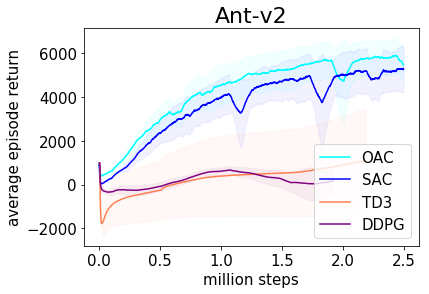
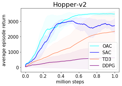
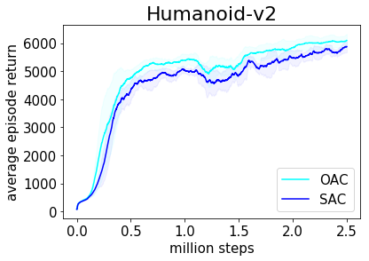
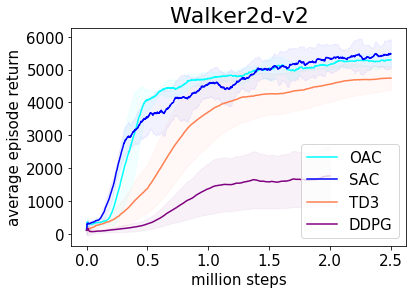
Our experiments have three main goals. First, to test whether Optimistic Actor Critic has performance competitive to state-of-the art algorithms. Second, to assess whether optimistic exploration based on the bootstrapped uncertainty estimate (24), is sufficient to produce a performance improvement. Third, to assess whether optimistic exploration adversely affects the stability of the learning process.

MuJoCo Continuous Control

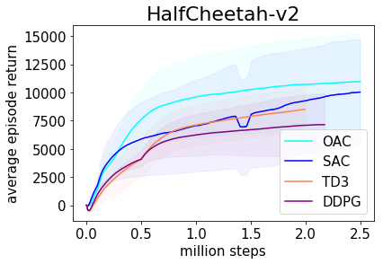
We test OAC on the MuJoCo [45] continuous control benchmarks. We compare OAC to SAC [25] and TD3 [17], two recent model-free RL methods that achieve state-of-the art performance. For completeness, we also include a comparison to a tuned version of DDPG [31], an established algorithm that does not maintain multiple bootstraps of the critic network. OAC uses 3 hyper-parameters related to exploration. The parameters $\beta_{\text{UB}}$ and $\beta_{\text{LB}}$ control the amount of uncertainty used to compute the upper and lower bound respectively. The parameter $\delta$ controls the maximal allowed divergence between the exploration policy and the target policy. We provide the values of all hyper-parameters and details of the hyper-parameter tuning in Appendix D. Results in Figure 3 show that using optimism improves the overall performance of actor-critic methods. On Ant, OAC improves the performance somewhat. On Hopper, OAC achieves state-of the art final performance. On Walker, we achieve the same performance as SAC while the high variance of results on HalfCheetah makes it difficult to draw conclusions on which algorithm performs better..

State-of-the art result on Humanoid

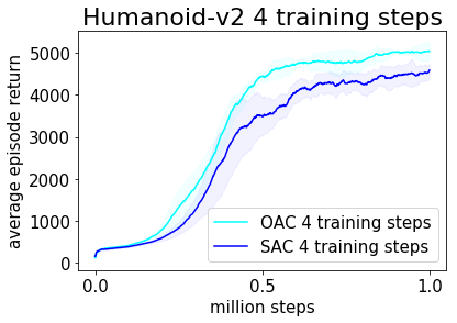
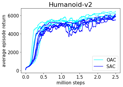
The upper-right plot of Figure 3 shows that the vanilla version of OAC outperforms SAC the on the Humanoid task. To test the statistical significance of our result, we re-ran both SAC and OAC in a setting where 4 training steps per iteration are used. By exploiting the memory buffer more fully, the 4-step versions show the benefit of improved exploration more clearly. The results are shown in the lower-right plot in Figure 3. At the end of training, the 90% confidence interval for the performance of OAC was $5033\pm 147$ while the performance of SAC was $4586\pm 117$. We stress that we did not tune hyper-parameters on the Humanoid environment. Overall, the fact that we are able to improve on Soft-Actor-Critic, which is currently the most sample-efficient model-free RL algorithm for continuous tasks shows that optimism can be leveraged to benefit sample efficiency. We provide an explicit plot of sample-efficiency in Appendix J.

Figure 4: Impact of the bootstrapped uncertainty estimate on the performance of OAC.

Figure 5: Left figure: individual runs of OAC vs SAC. Right figure: sensitivity to the KL constraint $\delta$. Error bars indicate $90\%$ confidence interval.

Usefulness of the Bootstrapped Uncertainty Estimate

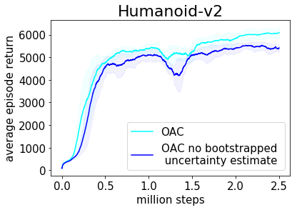
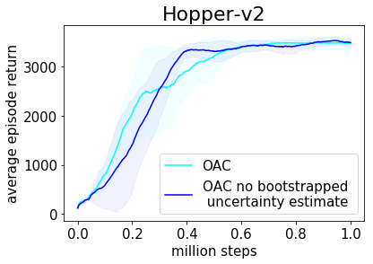
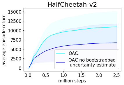
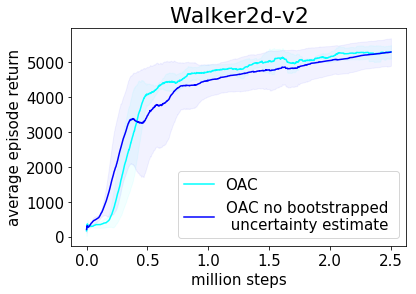
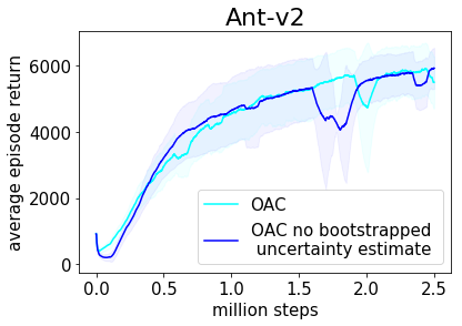
OAC uses an epistemic uncertainty estimate obtained using two bootstraps of the critic network. To investigate its benefit, we compare the performance of OAC to a modified version of the algorithm, which adjusts the exploration policy to maximize the approximate lower bound, replacing $\hat{Q}_{\text{UB}}$ with $\hat{Q}_{\text{LB}}$ in equation (9). While the modified algorithm does not use the uncertainty estimate, it still uses a shifted exploration policy, preferring actions that achieve higher state-action values. The results is shown in Figure 4 (we include more plots in Figure 8 in the Appendix). Using the bootstrapped uncertainty estimate improves performance on the most challenging Humanoid domain, while producing either a slight improvement or a no change in performance on others domains. Since the upper bound is computationally very cheap to obtain, we conclude that it is worthwhile to use it.

Sensitivity to the KL constraint

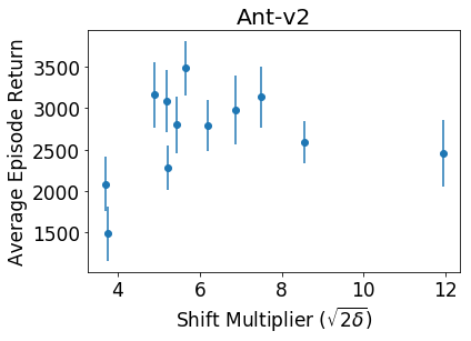
OAC relies on the hyperparameter $\delta$, which controls the maximum allowed KL divergence between the exploration policy and the target policy. In Figure 5, we evaluate how the term $\sqrt{2\delta}$ used in the the exploration policy (9) affects average performance of OAC trained for 1 million environment steps on the Ant-v2 domain. The results demonstrate that there is a broad range of settings for the hyperparameter $\delta$, which leads to good performance.

Learning is Stable in Practice

Since OAC explores with a shifted policy, it might at first be expected of having poorer learning stability relative to algorithms that use the target policy for exploration. While we have already shown above that the performance difference between OAC and SAC is statistically significant and not due to increased variance across runs, we now investigate stability further. In Figure 5 we compare individual learning runs across both algorithms. We conclude that OAC and SAC are similarly stable, avoiding the problems associated with stabilising deep off-policy RL [43, 47].

6 Conclusions

We present Optimistic Actor Critic (OAC), a model-free deep reinforcement learning algorithm which explores by maximizing an approximate confidence bound on the state-action value function. By addressing the inefficiencies of pessimistic underexploration and directional uninformedness, we are able to achieve state-of-the art sample efficiency in continuous control tasks. Our results suggest that the principle of optimism in the face of uncertainty can be used to improve the sample efficiency of policy gradient algorithms in a way which carries almost no additional computational overhead.

Better Exploration with Optimistic Actor-Critic

Appendices

A Proof of Proposition 1

Proposition 1.

The exploration policy resulting from (6) has the form $\pi_{E}=\mathcal{N}(\mu_{E},\Sigma_{E})$, where

$$\mu_{E}=\mu_{T}+\frac{\sqrt{2\delta}}{\scriptstyle\left\|\left[\nabla_{a}\hat{Q}_{\text{UB}}(s,a)\right]_{a=\mu_{T}}\right\|_{\Sigma_{T}}}\Sigma_{T}\left[\nabla_{a}\hat{Q}_{\text{UB}}(s,a)\right]_{a=\mu_{T}}\quad\text{and}\quad\Sigma_{E}=\Sigma_{T}.$$ (10)

Proof.

Consider the formula for the KL distance between two Gaussian distributions.

$$\operatorname*{KL}(\mathcal{N}(\mu,\Sigma),\mathcal{N}(\mu_{T},\Sigma_{T}))=\textstyle\frac{1}{2}\left(\operatorname*{tr}(\Sigma_{T}^{-1}\Sigma-I)+\log\frac{\det\Sigma_{T}}{\det\Sigma}+(\mu-\mu_{T})^{\top}\Sigma_{T}(\mu-\mu_{T})\right).$$ (11)

Consider the minimization problem

$$\min_{\Sigma}\operatorname*{KL}(\mathcal{N}(\mu,\Sigma),\mathcal{N}(\mu_{T},\Sigma_{T}))=\min_{\Sigma}\textstyle\frac{1}{2}\left(\operatorname*{tr}(\Sigma_{T}^{-1}\Sigma-I)+\log\frac{\det\Sigma_{T}}{\det\Sigma}\right).$$ (12)

The equality in (12) follows by eliminating a term in KL that does not depend on $\Sigma$. From the fact that KL divergence is non-negative and because the term under the minimum becomes zero when setting $\Sigma=\Sigma_{E}$, we obtain:

$$\Sigma_{E}=\min_{\Sigma}\textstyle\frac{1}{2}\left(\operatorname*{tr}(\Sigma_{T}^{-1}\Sigma-I)+\log\frac{\det\Sigma_{T}}{\det\Sigma}\right)=\Sigma_{T}.$$

Next, plugging $\Sigma_{E}=\Sigma_{T}$ into (6), we obtain the simpler optimization problem

$$\operatorname*{arg\,max}_{\mu:\atop\operatorname*{KL}(\mathcal{N}(\mu,\Sigma_{T}),\mathcal{N}(\mu_{T},\Sigma_{T}))\leq\delta}\bar{Q}_{\text{UB}}(s,\mu).$$ (13)

Using the formula for the KL divergence between Gaussian policies with the same covariance, $\operatorname*{KL}(\mathcal{N}(\mu,\Sigma_{T}),\mathcal{N}(\mu_{T},\Sigma_{T}))=\frac{1}{2}(\mu-\mu_{T})^{\top}\Sigma_{T}^{-1}(\mu-\mu_{T})$, we can write (13) as

$$\text{maximize}\;\;\bar{Q}_{\text{UB}}(s,\mu)\;\;\text{subject to}\;\;\frac{1}{2}(\mu-\mu_{T})^{\top}\Sigma_{T}^{-1}(\mu-\mu_{T})\leq\delta.$$ (14)

To solve the problem $\eqref{eq-mean-only-qf}$, we introduce the Lagrangian:

$$L=\bar{Q}_{\text{UB}}(s,\mu)-\lambda(\frac{1}{2}(\mu-\mu_{T})^{\top}\Sigma_{T}^{-1}(\mu-\mu_{T})-\delta).$$

Differentiating the Lagrangian, we get:

$$\nabla_{\mu}L=\left[\nabla_{a}\bar{Q}_{\text{UB}}(s,a)\right]_{a=\mu}-\lambda\Sigma_{T}^{-1}(\mu-\mu_{T})$$

Setting $\nabla_{\mu}L$ to zero, we obtain:

$$\mu=\frac{1}{\lambda}\Sigma_{T}\left[\nabla_{a}\bar{Q}_{\text{UB}}(s,a)\right]_{a=\mu}+\mu_{T}.$$ (15)

By enforcing the KKT conditions, we obtain $\lambda>0$ and

$$(\mu-\mu_{T})^{\top}\Sigma_{T}^{-1}(\mu-\mu_{T})=2\delta.$$ (16)

By plugging (15) into (16), we obtain

$$\lambda=\sqrt{\frac{\left[\nabla_{a}\bar{Q}_{\text{UB}}(s,a)\right]_{a=\mu_{T}}^{\top}\Sigma_{T}\left[\nabla_{a}\bar{Q}_{\text{UB}}(s,a)\right]_{a=\mu_{T}}}{2\delta}}=\frac{\scriptstyle\left\|\left[\nabla_{a}\bar{Q}_{\text{UB}}(s,a)\right]_{a=\mu_{T}}\right\|_{\Sigma_{T}}}{\sqrt{2\delta}}.$$ (17)

Plugging again into (15), we obtain the solution as

$$\mu_{E} =\mu_{T}+\frac{\sqrt{2\delta}}{\scriptstyle\left\|\left[\nabla_{a}\bar{Q}_{\text{UB}}(s,a)\right]_{a=\mu_{T}}\right\|_{\Sigma_{T}}}\Sigma_{T}\left[\nabla_{a}\bar{Q}_{\text{UB}}(s,a)\right]_{a=\mu}=$$ (18)

$$=\mu_{T}+\frac{\sqrt{2\delta}}{\scriptstyle\left\|\left[\nabla_{a}\hat{Q}_{\text{UB}}(s,a)\right]_{a=\mu_{T}}\right\|_{\Sigma_{T}}}\Sigma_{T}\left[\nabla_{a}\hat{Q}_{\text{UB}}(s,a)\right]_{a=\mu}.$$ (19)

Here, the last equality follows from (8). ∎

B Deterministic version of OAC

In response to feedback following the initial version of OAC, we developed a variant that explores using a deterministic policy. While using a deterministic policy for exploration may appear surprising, deterministic OAC works because taking an action that maximises an upper bound of the critic is often a better choice than taking the action that maximises the mean estimate. Formally, deterministic OAC explores with a policy that solves the optimization problem

$$\mu_{E}=\operatorname*{arg\,max}_{\mu:\atop\operatorname*{W}(\delta(\mu),\delta(\mu_{T}))\leq\delta}\bar{Q}_{\text{UB}}(s,\mu).$$ (20)

Here, we denote a deterministic probability distribution (Dirac delta) centred at $a$ with $\delta(a)$. We used the Wasserstein divergence (denoted with $\operatorname*{W}$) because the KL metric becomes singular for deterministic policies. Below, we derive a result that provides us with an explicit form of the exploration policy for deterministic OAC, analogous to Proposition 1.

Proposition 2.

The exploration policy resulting from (20) has the form $\pi_{E}=\delta(\mu_{E})$, where

$$\mu_{E}=\mu_{T}+\frac{\sqrt{2\delta}}{\scriptstyle\left\|\left[\nabla_{a}\hat{Q}_{\text{UB}}(s,a)\right]_{a=\mu_{T}}\right\|}\left[\nabla_{a}\hat{Q}_{\text{UB}}(s,a)\right]_{a=\mu_{T}}.$$ (21)

Proof.

Consider the formula for the Wasserstein divergence between two Dirac-delta distributions.

$$\operatorname*{W}(\delta(\mu),\delta(\mu_{T}))=\textstyle\frac{1}{2}\left\|\mu-\mu_{T}\right\|^{2}.$$ (22)

Plugging this into 20 leads to the optimization problem

$$\text{maximise}\;\;\bar{Q}_{\text{UB}}(s,\mu)\;\;\text{subject to}\;\;\frac{1}{2}(\mu-\mu_{T})^{\top}(\mu-\mu_{T})\leq\delta.$$ (23)

The rest of the proof follows analogously to the proof of Poposition 1, by observing that equation (23) is a special case of (14). ∎

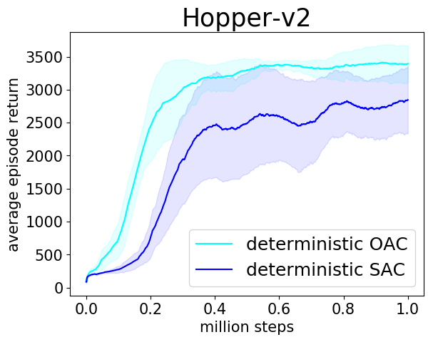
The deterministic version of OAC is identical to regular OAC except for using the exploration policy from Proposition 2. An example experiment is shown in Figure 6.

Figure 6: Experiment showing the performance of a deterministic version of OAC.

C Population standard deviation of two values

For completeness, we include the computation of the population standard deviation of two values. Consider a two-element sample $\{\hat{Q}_{\text{LB}}^{1}(s,a),\hat{Q}_{\text{LB}}^{2}(s,a)\}$. Denote the sample mean by $\mu_{Q}(s,a)=\frac{1}{2}(\hat{Q}_{\text{LB}}^{1}(s,a)+\hat{Q}_{\text{LB}}^{2}(s,a))$. The population standard deviation takes the form

$$\sigma_{Q}(s,a) =\sqrt{\sum_{i\in\{1,2\}}\frac{1}{2}\left(\hat{Q}_{\text{LB}}^{i}(s,a)-\mu_{Q}(s,a)\right)^{2}}$$ (24)

$$=\sqrt{\frac{1}{2}\left(\frac{1}{2}\hat{Q}_{\text{LB}}^{1}(s,a)-\frac{1}{2}\hat{Q}_{\text{LB}}^{2}(s,a)\right)^{2}+\frac{1}{2}\left(\frac{1}{2}\hat{Q}_{\text{LB}}^{1}(s,a)-\frac{1}{2}\hat{Q}_{\text{LB}}^{2}(s,a)\right)^{2}}$$ (25)

$$=\sqrt{\left(\frac{1}{2}\hat{Q}_{\text{LB}}^{1}(s,a)-\frac{1}{2}\hat{Q}_{\text{LB}}^{2}(s,a)\right)^{2}}$$ (26)

$$=\frac{1}{2}\sqrt{\left(\hat{Q}_{\text{LB}}^{1}(s,a)-\hat{Q}_{\text{LB}}^{2}(s,a)\right)^{2}}$$ (27)

$$=\frac{1}{2}\left|\hat{Q}_{\text{LB}}^{1}(s,a)-\hat{Q}_{\text{LB}}^{2}(s,a)\right|$$ (28)

From this formula, we can obtain:

$$\mu_{Q}(s,a)-\sigma_{Q}(s,a) =\frac{1}{2}(\hat{Q}_{\text{LB}}^{1}(s,a)+\hat{Q}_{\text{LB}}^{2}(s,a))-\frac{1}{2}\left|\hat{Q}_{\text{LB}}^{1}(s,a)-\hat{Q}_{\text{LB}}^{2}(s,a)\right|$$ (29)

$$=\min(\hat{Q}_{\text{LB}}^{1}(s,a),\hat{Q}_{\text{LB}}^{2}(s,a)).$$ (30)

This formula allows us to interpret the minimization used by TD3 [17] and SAC [24] as an approximate lower confidence bound. Similarly, we have:

$$\mu_{Q}(s,a)+\sigma_{Q}(s,a)=\max(\hat{Q}_{\text{LB}}^{1}(s,a),\hat{Q}_{\text{LB}}^{2}(s,a)).$$ (31)

This indicates that using UCB with $\beta_{UB}=1$ is equivalent to taking the maximum of the two critics.

D Experimental setup and hyper-parameters

Our learning curves show the total undiscounted return. Following the convention of SAC, we smoothen the curves, so the y-value at any point corresponds to the average across the last 100 data points.

Our implementation was based on softlearning, the official SAC implementation [25] . All experiments for OAC and SAC were run within Docker containers on CPU-only $Standard\_D8s\_v3$ machine type on Azure Cloud.

We made the following modifications to the evaluation:

1. In addition to setting the initial seeds of the computational packages used (NumPy, Tensorflow  [1]), we also fix the seeds of the environments to ensure reproducibility of results given initial seed values. In practice, the seed of the environment controls the initial state distribution.

2. Instead of randomly sampling training and evaluation seeds, we force the seeds to come from disjoint sets.

We list OAC-specific hyper-parameters in Table 1 and 2. The other parameters were set as provided in the implementation of the Soft Actor-Critic algorithms from the softlearning repository . We list them in Appendix E for completeness.

Table 1: OAC Hyperparameters when training with 1 training gradient per environment step

Parameter		Value	Range used for tuning
	shift multiplier $\sqrt{2\delta}$	$6.86$	$[0,12]$
	$\beta_{\text{UB}}$	$4.66$	$[0,7]$
	$\beta_{\text{LB}}$	$-3.65$	$[-7,-1]$

Table 2: OAC Hyperparameters when training with 4 gradient steps per environment step

Parameter		Value	Range used for tuning
	shift multiplier $\sqrt{2\delta}$	$3.69$	$[0,12]$
	$\beta_{\text{UB}}$	$4.36$	$[0,7]$
	$\beta_{\text{LB}}$	$-2.54$	$[-7,-1]$
	target smoothing coefficient ($\tau$)	$0.003$	$[0.001,0.005]$

The OAC hyper-parameters have been tuned on four Mujoco environments (Ant-v2, Walker2d-v2, HalfCheetah-v2, Hopper-v2), using Bayesian optimization with parameter ranges given in Table 1 and 2. We used the average performance over the first 250 thousand steps of the algorithm as the BO optimization metric. Dusring BO, we sampled 1 hyperparameter setting at a time and performed an experiment on a single seed. We did not tune hyperparameters on Humanoid-v2.

E Reproducing the Baselines

Table 3: SAC Hyperparameters

Parameter		Value
	optimizer	Adam [30]
	learning rate	$3\cdot 10^{-4}$
	discount ($\gamma$)	$0.99$
	replay buffer size	$10^{6}$
	number of hidden layers (all networks)	2
	number of hidden units per layer	256
	number of samples per minibatch	256
	nonlinearity	ReLU
	target smoothing coefficient ($\tau$)	$0.005$
	target update interval	1
	gradient steps	1

Table 4: TD3 Hyperparameters (From [17])

Parameter		Value
	critic learning rate	$0.0003$
	actor learning rate	$0.0003$
	optimizer	Adam [30]
	target smoothing coefficient ($\tau$)	0.005
	target update interval	1
	policy frequency	2
	policy noise	0.2
	noise clipping threshold	0.5
	number of samples per minibatch	100
	gradient steps	1
	discount ($\gamma$)	0.99
	replay buffer size	$10^{6}$
	number of hidden layers (all networks)	1
	number of units per hidden layer	256
	nonlinearity	ReLU
	exploration policy	$\mathcal{N}(0,0.1)$

Table 5: DDPG Hyperparameters (From [17])

Parameter		Value
	critic learning rate	$0.001$
	actor learning rate	$0.001$
	optimizer	Adam [30]
	target smoothing coefficient ($\tau$)	0.005
	target update interval	1
	number of samples per minibatch	100
	gradient steps	1
	discount ($\gamma$)	0.99
	replay buffer size	$10^{6}$
	number of hidden layers (all networks)	2
	number of units per hidden layer (from first to last)	400, 300
	nonlinearity	ReLU
	exploration policy	$\mathcal{N}(0,0.1)$
	number of training runs	$5$

Soft-Actor Critic

SAC results are obtained by running official SAC implementation [25] from the softlearning repository. Additionally, to ensure reproducibility, we made the same changes to the evaluation setup that were discussed in Appendix D. The SAC results we obtained are similar to previously reported results [25], except on HalfCheetah-v2. The performance of SAC on HalfCheetah-v2 in Figure 3 does not match the performance reported in [25]. This is because performance on this environment has high variance. We have also confirmed this observation with the SAC authors.

TD3 and DDPG

The official implementation of TD3 (https://github.com/sfujim/TD3) was used to generate the baselines in Figure 3. Similarly, the tuned DDPG implementation we use is the ‘OurDDPG’ baseline used in [17].

F Visualisations of the critic for continuous control domains

Figure 7: Visualization of the critic lower bound (red curve) and the action distribution for a given state. The policy mean $\mu$ is denoted by the light blue dot. Each of the 6 plot shows the values of the critic for a different state seen by the SAC agent training on Ant-v2.

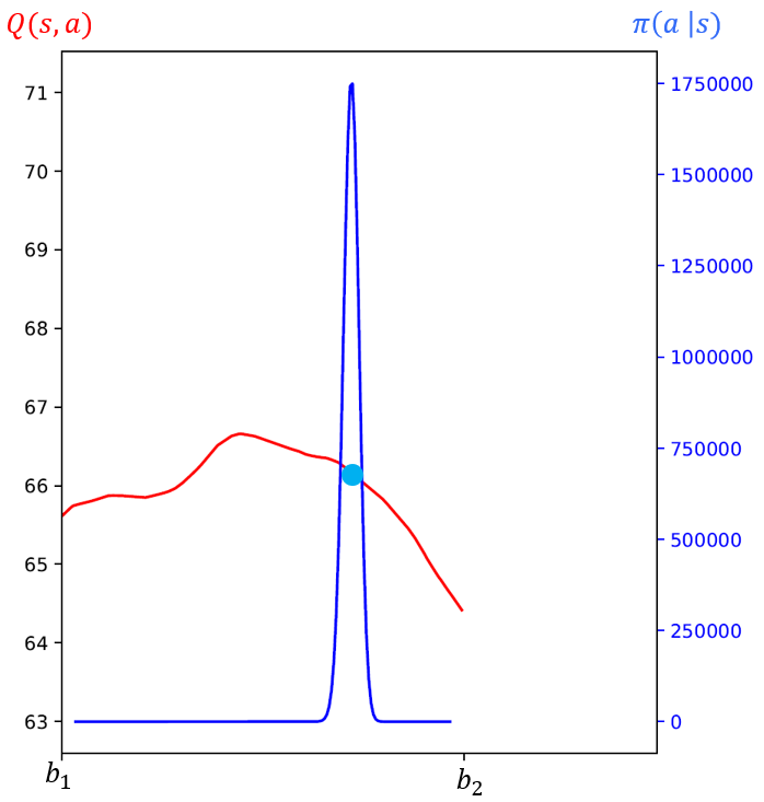
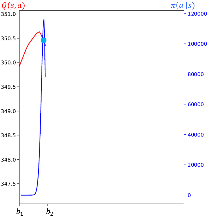
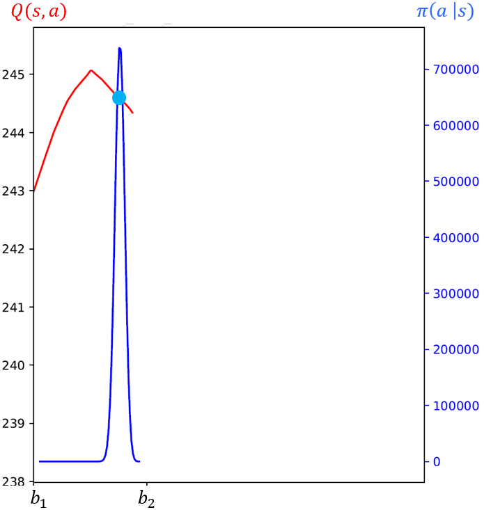
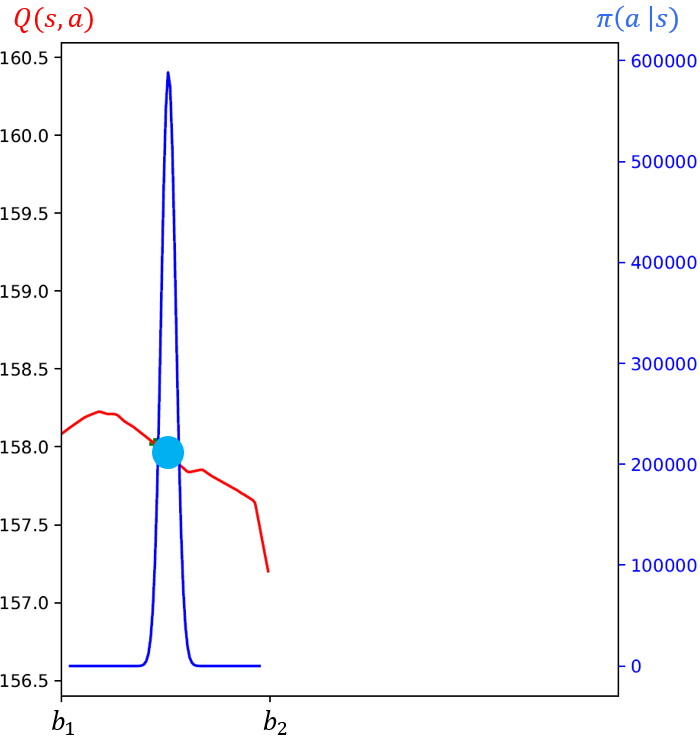
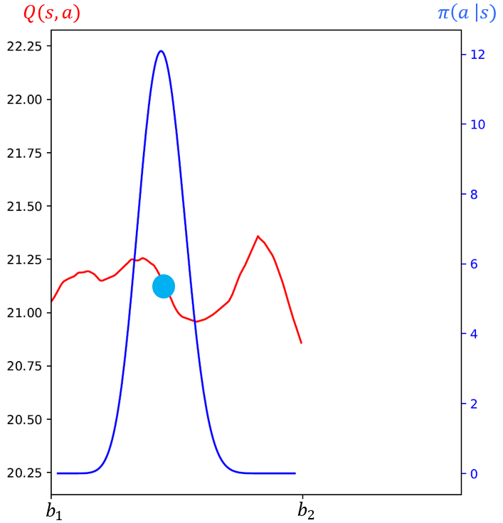
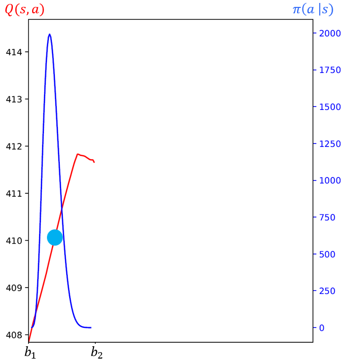
Figure 7 shows the visualization of the critic lower bound and the policy during training. The 6 states used to plot were sampled randomly and come from the different training runs of Ant-v2. The second figure in the first row demonstrates the phenomenon of pessimistic underexploration in practice. The plots were obtained by intersecting a ray cast from the policy mean $\mu$ in a random direction with the hypercube defining the valid action range.

G Ablations

Figure 8 shows plots demonstrating the difference in the performance of OAC with and without the bootstrapped uncertainty estimate for all 5 domains.

Figure 8: Ablation studies for OAC on the benefit of the critic’s approximate upper bound.

H Policy gradient algorithms are greedy

Figure 9: Policy variance as a function of time, when applying policy gradients to a continuous bandit problem.

In this section, we recall existing analytic results [13, 14] to provide more background about how policy gradient methods behave asymptotically. Following [14], we show the behavior of policy gradients on a simple task where the critic is a quadratic function, given by $\hat{Q}=-a^{2}$. In order to abstract away the effects of simulation noise, we use Expected Policy Gradients, a variance-free policy gradient algorithm where the policy at each step can be obtained analytically. In Figure 9, we can see the policy variance as a function of optimization time-step. The fact that $\sigma^{2}$ decays to zero is consistent with the intuition that the function $-a^{2}$ has one optimum $a=0$. The optimal policy simply puts an increasing amount of probability mass in that optimum. We empirically demonstrate in the middle plot in the upper row of Figure 7 that a similar phenomenon is happening with soft actor-critic. Since policy gradients are fundamentally optimization algorithms that maximize the critic, the policy covariance still becomes very small in the optima of the critic, despite entropy regularization and noisy sampling of actions used by SAC. While maximising the critic is actually a good thing if the critic is accurate, it leads to pessimistic under-exploration when we only have a loose lower bound. OAC addresses this problem by using a modified exploration policy.

I Upper bound encourages exploration

(a) Lower bound worse than upper bound for exploration.

(b) Smooth upper bound tight in a region near $\mu$ (here: to the right) cannot have a spurious local maximum at $\mu$.

Figure 10: Properties of the critic upper and lower bound for exploration.

We give more intuitions about how using a lower bound of the critic inhibits exploration, while using an upper bound encourages it. Figure 10(a) shows the true critic, a lower bound and an upper bound for a one-dimensional continuous bandit problem. If we use the lower bound $\hat{Q}_{\text{LB}}$ for updating the policy, the standard deviation of the policy becomes small as described above, since we have a local maximum. On the other hand, using the upper bound $\hat{Q}_{\text{UB}}$, we have a moderate standard deviation and a strong policy gradient for the mean, meaning the policy doesn’t get stuck. At first, one may think that the example in Figure 10(a) is cherry-picked since the upper bound may also have a spurious local maximum. However, Figure 10(b) demonstrates that it cannot be the case. A smooth function cannot simultaneously track the true critic in some region close to $\mu$, have a spurious maximum at $\mu$ and be an upper bound.

J Plot of sample efficiency

Figure 11: Explicit Plot of Sample Efficiency

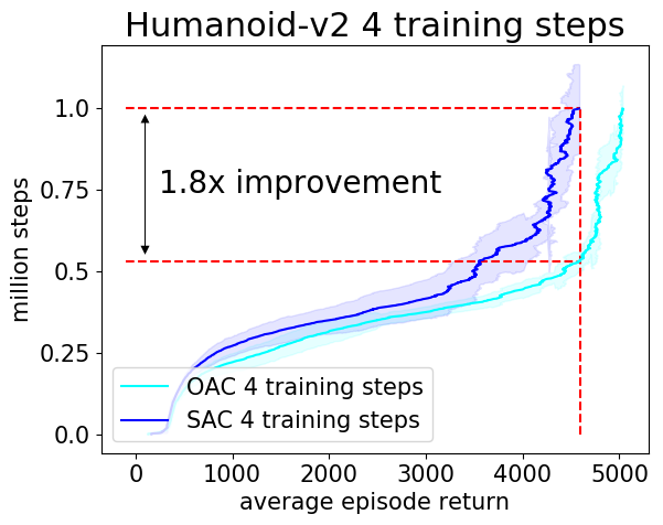
Figure 11 shows the number of steps required to achieve a given level of performance.

K Additional ablations

(a) Amount of policy shift at a given timestep.

(b) Effect of the optimism parameter $\beta_{UB}$.

Figure 12: Additional ablations.

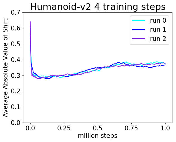
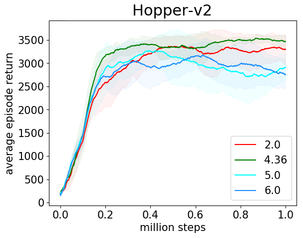
Figure 12(a) shows the shift, i.e. the norm of the difference between the mean of the target policy $\pi_{T}$ and the exploration policy $\pi_{E}$. The reported value is averaged across a single minibatch.

Figure 12(b) shows learning curves for four different values of $\beta_{UB}$, including the sweet-spot value of 4.36 that was used for the final result.

References

- Abadi et al. [2016] Martín Abadi, Ashish Agarwal, Paul Barham, Eugene Brevdo, Zhifeng Chen, Craig Citro, Gregory S. Corrado, Andy Davis, Jeffrey Dean, Matthieu Devin, Sanjay Ghemawat, Ian J. Goodfellow, Andrew Harp, Geoffrey Irving, Michael Isard, Yangqing Jia, Rafal Józefowicz, Lukasz Kaiser, Manjunath Kudlur, Josh Levenberg, Dan Mané, Rajat Monga, Sherry Moore, Derek Gordon Murray, Chris Olah, Mike Schuster, Jonathon Shlens, Benoit Steiner, Ilya Sutskever, Kunal Talwar, Paul A. Tucker, Vincent Vanhoucke, Vijay Vasudevan, Fernanda B. Viégas, Oriol Vinyals, Pete Warden, Martin Wattenberg, Martin Wicke, Yuan Yu, and Xiaoqiang Zheng. Tensorflow: Large-scale machine learning on heterogeneous distributed systems. CoRR, abs/1603.04467, 2016. URL http://arxiv.org/abs/1603.04467.
- Abdolmaleki et al. [2015] Abbas Abdolmaleki, Rudolf Lioutikov, Jan R Peters, Nuno Lau, Luis Pualo Reis, and Gerhard Neumann. Model-Based Relative Entropy Stochastic Search. In C. Cortes, N. D. Lawrence, D. D. Lee, M. Sugiyama, and R. Garnett, editors, Advances in Neural Information Processing Systems 28, pages 3537–3545. Curran Associates, Inc., 2015.
- Abdolmaleki et al. [2018] Abbas Abdolmaleki, Jost Tobias Springenberg, Yuval Tassa, Rémi Munos, Nicolas Heess, and Martin A. Riedmiller. Maximum a Posteriori Policy Optimisation. In 6th International Conference on Learning Representations, ICLR 2018, Vancouver, BC, Canada, April 30 - May 3, 2018, Conference Track Proceedings. OpenReview.net, 2018.
- Akrour et al. [2016] Riad Akrour, Gerhard Neumann, Hany Abdulsamad, and Abbas Abdolmaleki. Model-Free Trajectory Optimization for Reinforcement Learning. In Maria-Florina Balcan and Kilian Q. Weinberger, editors, Proceedings of the 33nd International Conference on Machine Learning, ICML 2016, New York City, NY, USA, June 19-24, 2016, volume 48 of JMLR Workshop and Conference Proceedings, pages 2961–2970. JMLR.org, 2016.
- Amari [1998] Shun-ichi Amari. Natural Gradient Works Efficiently in Learning. Neural Computation, 10(2):251–276, 1998. doi: 10.1162/089976698300017746.
- Baxter and Bartlett [2000] J. Baxter and P. L. Bartlett. Direct gradient-based reinforcement learning. In IEEE International Symposium on Circuits and Systems, ISCAS 2000, Emerging Technologies for the 21st Century, Geneva, Switzerland, 28-31 May 2000, Proceedings, pages 271–274. IEEE, 2000. doi: 10.1109/ISCAS.2000.856049.
- Baxter and Bartlett [2001] Jonathan Baxter and Peter L. Bartlett. Infinite-Horizon Policy-Gradient Estimation. J. Artif. Intell. Res., 15:319–350, 2001. doi: 10.1613/jair.806.
- Baxter et al. [2001] Jonathan Baxter, Peter L. Bartlett, and Lex Weaver. Experiments with Infinite-Horizon, Policy-Gradient Estimation. J. Artif. Intell. Res., 15:351–381, 2001. doi: 10.1613/jair.807.
- Brafman and Tennenholtz [2002] Ronen I. Brafman and Moshe Tennenholtz. R-max-a general polynomial time algorithm for near-optimal reinforcement learning. Journal of Machine Learning Research, 3(Oct):213–231, 2002.
- Callahan [2010] James J. Callahan. Advanced Calculus: A Geometric View. Springer Science & Business Media, September 2010. ISBN 978-1-4419-7332-0.
- Chen et al. [2017] Richard Y Chen, Szymon Sidor, Pieter Abbeel, and John Schulman. Ucb exploration via q-ensembles. arXiv preprint arXiv:1706.01502, 2017.
- Chua et al. [2018] Kurtland Chua, Roberto Calandra, Rowan McAllister, and Sergey Levine. Deep reinforcement learning in a handful of trials using probabilistic dynamics models. In Advances in Neural Information Processing Systems 31: Annual Conference on Neural Information Processing Systems 2018, NeurIPS 2018, 3-8 December 2018, Montréal, Canada., pages 4759–4770, 2018. URL http://papers.nips.cc/paper/7725-deep-reinforcement-learning-in-a-handful-of-trials-using-probabilistic-dynamics-models.
- Ciosek and Whiteson [2018a] Kamil Ciosek and Shimon Whiteson. Expected Policy Gradients. In Sheila A. McIlraith and Kilian Q. Weinberger, editors, Proceedings of the Thirty-Second AAAI Conference on Artificial Intelligence, (AAAI-18), the 30th Innovative Applications of Artificial Intelligence (IAAI-18), and the 8th AAAI Symposium on Educational Advances in Artificial Intelligence (EAAI-18), New Orleans, Louisiana, USA, February 2-7, 2018, pages 2868–2875. AAAI Press, 2018a.
- Ciosek and Whiteson [2018b] Kamil Ciosek and Shimon Whiteson. Expected Policy Gradients for Reinforcement Learning. CoRR, abs/1801.03326, 2018b.
- Depeweg et al. [2016] Stefan Depeweg, José Miguel Hernández-Lobato, Finale Doshi-Velez, and Steffen Udluft. Learning and policy search in stochastic dynamical systems with bayesian neural networks. arXiv preprint arXiv:1605.07127, 2016.
- Efron and Tibshirani [1994] Bradley Efron and Robert J. Tibshirani. An Introduction to the Bootstrap. SIAM Review, 36(4):677–678, 1994. doi: 10.1137/1036171.
- Fujimoto et al. [2018] Scott Fujimoto, Herke Hoof, and David Meger. Addressing Function Approximation Error in Actor-Critic Methods. In International Conference on Machine Learning, pages 1582–1591, 2018.
- Gal et al. [2016] Yarin Gal, Rowan McAllister, and Carl Edward Rasmussen. Improving pilco with bayesian neural network dynamics models. In Data-Efficient Machine Learning workshop, ICML, volume 4, 2016.
- Ghavamzadeh and Engel [2007] Mohammad Ghavamzadeh and Yaakov Engel. Bayesian actor-critic algorithms. In Machine Learning, Proceedings of the Twenty-Fourth International Conference (ICML 2007), Corvallis, Oregon, USA, June 20-24, 2007, pages 297–304, 2007. doi: 10.1145/1273496.1273534. URL https://doi.org/10.1145/1273496.1273534.
- Ghavamzadeh et al. [2015] Mohammad Ghavamzadeh, Shie Mannor, Joelle Pineau, and Aviv Tamar. Bayesian reinforcement learning: A survey. Foundations and Trends in Machine Learning, 8(5-6):359–483, 2015. doi: 10.1561/2200000049. URL https://doi.org/10.1561/2200000049.
- Ghavamzadeh et al. [2016] Mohammad Ghavamzadeh, Yaakov Engel, and Michal Valko. Bayesian policy gradient and actor-critic algorithms. Journal of Machine Learning Research, 17:66:1–66:53, 2016. URL http://jmlr.org/papers/v17/10-245.html.
- Gu et al. [2017a] Shixiang Gu, Tim Lillicrap, Richard E. Turner, Zoubin Ghahramani, Bernhard Schölkopf, and Sergey Levine. Interpolated Policy Gradient: Merging On-Policy and Off-Policy Gradient Estimation for Deep Reinforcement Learning. In Isabelle Guyon, Ulrike von Luxburg, Samy Bengio, Hanna M. Wallach, Rob Fergus, S. V. N. Vishwanathan, and Roman Garnett, editors, Advances in Neural Information Processing Systems 30: Annual Conference on Neural Information Processing Systems 2017, 4-9 December 2017, Long Beach, CA, USA, pages 3849–3858, 2017a.
- Gu et al. [2017b] Shixiang Gu, Timothy P. Lillicrap, Zoubin Ghahramani, Richard E. Turner, and Sergey Levine. Q-Prop: Sample-Efficient Policy Gradient with An Off-Policy Critic. In 5th International Conference on Learning Representations, ICLR 2017, Toulon, France, April 24-26, 2017, Conference Track Proceedings. OpenReview.net, 2017b.
- Haarnoja et al. [2018a] Tuomas Haarnoja, Aurick Zhou, Pieter Abbeel, and Sergey Levine. Soft Actor-Critic: Off-Policy Maximum Entropy Deep Reinforcement Learning with a Stochastic Actor. In International Conference on Machine Learning, pages 1856–1865, 2018a.
- Haarnoja et al. [2018b] Tuomas Haarnoja, Aurick Zhou, Kristian Hartikainen, George Tucker, Sehoon Ha, Jie Tan, Vikash Kumar, Henry Zhu, Abhishek Gupta, Pieter Abbeel, and Sergey Levine. Soft Actor-Critic Algorithms and Applications. CoRR, abs/1812.05905, 2018b.
- Hasselt [2010] Hado V. Hasselt. Double Q-learning. In Advances in Neural Information Processing Systems, pages 2613–2621, 2010.
- Heess et al. [2015] Nicolas Heess, Gregory Wayne, David Silver, Timothy P. Lillicrap, Tom Erez, and Yuval Tassa. Learning Continuous Control Policies by Stochastic Value Gradients. In Corinna Cortes, Neil D. Lawrence, Daniel D. Lee, Masashi Sugiyama, and Roman Garnett, editors, Advances in Neural Information Processing Systems 28: Annual Conference on Neural Information Processing Systems 2015, December 7-12, 2015, Montreal, Quebec, Canada, pages 2944–2952, 2015.
- Jin et al. [2018] Chi Jin, Zeyuan Allen-Zhu, Sébastien Bubeck, and Michael I. Jordan. Is Q-Learning Provably Efficient? In Samy Bengio, Hanna M. Wallach, Hugo Larochelle, Kristen Grauman, Nicolò Cesa-Bianchi, and Roman Garnett, editors, Advances in Neural Information Processing Systems 31: Annual Conference on Neural Information Processing Systems 2018, NeurIPS 2018, 3-8 December 2018, Montréal, Canada, pages 4868–4878, 2018.
- Kakade [2001] Sham Kakade. A Natural Policy Gradient. In Thomas G. Dietterich, Suzanna Becker, and Zoubin Ghahramani, editors, Advances in Neural Information Processing Systems 14 [Neural Information Processing Systems: Natural and Synthetic, NIPS 2001, December 3-8, 2001, Vancouver, British Columbia, Canada], pages 1531–1538. MIT Press, 2001.
- Kingma and Ba [2015] Diederik P. Kingma and Jimmy Ba. Adam: A method for stochastic optimization. In 3rd International Conference on Learning Representations, ICLR 2015, San Diego, CA, USA, May 7-9, 2015, Conference Track Proceedings, 2015. URL http://arxiv.org/abs/1412.6980.
- Lillicrap et al. [2016] Timothy P. Lillicrap, Jonathan J. Hunt, Alexander Pritzel, Nicolas Heess, Tom Erez, Yuval Tassa, David Silver, and Daan Wierstra. Continuous control with deep reinforcement learning. In Yoshua Bengio and Yann LeCun, editors, 4th International Conference on Learning Representations, ICLR 2016, San Juan, Puerto Rico, May 2-4, 2016, Conference Track Proceedings, 2016.
- Lim et al. [2018] Sungsu Lim, Ajin Joseph, Lei Le, Yangchen Pan, and Martha White. Actor-expert: A framework for using action-value methods in continuous action spaces. CoRR, abs/1810.09103, 2018. URL http://arxiv.org/abs/1810.09103.
- Mnih et al. [2015] Volodymyr Mnih, Koray Kavukcuoglu, David Silver, Andrei A. Rusu, Joel Veness, Marc G. Bellemare, Alex Graves, Martin A. Riedmiller, Andreas Fidjeland, Georg Ostrovski, Stig Petersen, Charles Beattie, Amir Sadik, Ioannis Antonoglou, Helen King, Dharshan Kumaran, Daan Wierstra, Shane Legg, and Demis Hassabis. Human-level control through deep reinforcement learning. Nature, 518(7540):529–533, 2015. doi: 10.1038/nature14236.
- O’Donoghue et al. [2018] Brendan O’Donoghue, Ian Osband, Rémi Munos, and Volodymyr Mnih. The uncertainty bellman equation and exploration. In Proceedings of the 35th International Conference on Machine Learning, ICML 2018, Stockholmsmässan, Stockholm, Sweden, July 10-15, 2018, pages 3836–3845, 2018. URL http://proceedings.mlr.press/v80/o-donoghue18a.html.
- Osband et al. [2016] Ian Osband, Charles Blundell, Alexander Pritzel, and Benjamin Van Roy. Deep Exploration via Bootstrapped DQN. In Daniel D. Lee, Masashi Sugiyama, Ulrike von Luxburg, Isabelle Guyon, and Roman Garnett, editors, Advances in Neural Information Processing Systems 29: Annual Conference on Neural Information Processing Systems 2016, December 5-10, 2016, Barcelona, Spain, pages 4026–4034, 2016.
- Osband et al. [2018] Ian Osband, John Aslanides, and Albin Cassirer. Randomized prior functions for deep reinforcement learning. In Advances in Neural Information Processing Systems 31: Annual Conference on Neural Information Processing Systems 2018, NeurIPS 2018, 3-8 December 2018, Montréal, Canada., pages 8626–8638, 2018. URL http://papers.nips.cc/paper/8080-randomized-prior-functions-for-deep-reinforcement-learning.
- Peters and Schaal [2006] Jan Peters and Stefan Schaal. Policy Gradient Methods for Robotics. In 2006 IEEE/RSJ International Conference on Intelligent Robots and Systems, IROS 2006, October 9-15, 2006, Beijing, China, pages 2219–2225. IEEE, 2006. ISBN 978-1-4244-0258-8. doi: 10.1109/IROS.2006.282564.
- Peters and Schaal [2008] Jan Peters and Stefan Schaal. Natural Actor-Critic. Neurocomputing, 71(7-9):1180–1190, 2008. doi: 10.1016/j.neucom.2007.11.026.
- Puterman [2014] Martin L. Puterman. Markov Decision Processes: Discrete Stochastic Dynamic Programming. John Wiley & Sons, 2014.
- Silver et al. [2014] David Silver, Guy Lever, Nicolas Heess, Thomas Degris, Daan Wierstra, and Martin A. Riedmiller. Deterministic Policy Gradient Algorithms. In Proceedings of the 31th International Conference on Machine Learning, ICML 2014, Beijing, China, 21-26 June 2014, volume 32 of JMLR Workshop and Conference Proceedings, pages 387–395. JMLR.org, 2014.
- Sutton [1995] Richard S. Sutton. Generalization in Reinforcement Learning: Successful Examples Using Sparse Coarse Coding. In David S. Touretzky, Michael Mozer, and Michael E. Hasselmo, editors, Advances in Neural Information Processing Systems 8, NIPS, Denver, CO, USA, November 27-30, 1995, pages 1038–1044. MIT Press, 1995. ISBN 978-0-262-20107-0.
- Sutton [1996] Richard S Sutton. Generalization in Reinforcement Learning: Successful Examples Using Sparse Coarse Coding. In D. S. Touretzky, M. C. Mozer, and M. E. Hasselmo, editors, Advances in Neural Information Processing Systems 8, pages 1038–1044. MIT Press, 1996.
- Sutton and Barto [2018] Richard S. Sutton and Andrew G. Barto. Reinforcement Learning: An Introduction. The MIT Press, second edition, 2018.
- Sutton et al. [1999] Richard S. Sutton, David A. McAllester, Satinder P. Singh, and Yishay Mansour. Policy Gradient Methods for Reinforcement Learning with Function Approximation. In Sara A. Solla, Todd K. Leen, and Klaus-Robert Müller, editors, Advances in Neural Information Processing Systems 12, [NIPS Conference, Denver, Colorado, USA, November 29 - December 4, 1999], pages 1057–1063. The MIT Press, 1999. ISBN 978-0-262-19450-1.
- Todorov et al. [2012] Emanuel Todorov, Tom Erez, and Yuval Tassa. MuJoCo: A physics engine for model-based control. 2012 IEEE/RSJ International Conference on Intelligent Robots and Systems, pages 5026–5033, 2012.
- van Hasselt et al. [2016] Hado van Hasselt, Arthur Guez, and David Silver. Deep Reinforcement Learning with Double Q-Learning. In Dale Schuurmans and Michael P. Wellman, editors, Proceedings of the Thirtieth AAAI Conference on Artificial Intelligence, February 12-17, 2016, Phoenix, Arizona, USA, pages 2094–2100. AAAI Press, 2016. ISBN 978-1-57735-760-5.
- van Hasselt et al. [2018] Hado van Hasselt, Yotam Doron, Florian Strub, Matteo Hessel, Nicolas Sonnerat, and Joseph Modayil. Deep Reinforcement Learning and the Deadly Triad. CoRR, abs/1812.02648, 2018.
- van Seijen et al. [2009] Harm van Seijen, Hado van Hasselt, Shimon Whiteson, and Marco A. Wiering. A theoretical and empirical analysis of Expected Sarsa. In IEEE Symposium on Adaptive Dynamic Programming and Reinforcement Learning, ADPRL 2009, Nashville, TN, USA, March 31 - April 1, 2009, pages 177–184. IEEE, 2009. ISBN 978-1-4244-2761-1. doi: 10.1109/ADPRL.2009.4927542.
- Williams [1992] Ronald J. Williams. Simple Statistical Gradient-Following Algorithms for Connectionist Reinforcement Learning. Machine Learning, 8:229–256, 1992. doi: 10.1007/BF00992696.
- Ziebart [2010] Brian D. Ziebart. Modeling Purposeful Adaptive Behavior with the Principle of Maximum Causal Entropy. PhD Thesis, Carnegie Mellon University, Pittsburgh, PA, USA, 2010.