Online Trajectory Planning Through Combined Trajectory Optimization and Function Approximation: Application to the Exoskeleton Atalante

Abstract

Autonomous robots require online trajectory planning capability to operate in the real world. Efficient offline trajectory planning methods already exist, but are computationally demanding, preventing their use online. In this paper, we present a novel algorithm called Guided Trajectory Learning that learns a function approximation of solutions computed through trajectory optimization while ensuring accurate and reliable predictions. This function approximation is then used online to generate trajectories. This algorithm is designed to be easy to implement, and practical since it does not require massive computing power. It is readily applicable to any robotics systems and effortless to set up on real hardware since robust control strategies are usually already available. We demonstrate the computational performance of our algorithm on flat-foot walking with the self-balanced exoskeleton Atalante.

I INTRODUCTION

Online trajectory planning enables robots to deal with a real-world environment that may change suddenly, and to carry out sequences of tasks in unknown orders and contexts. For instance, walking robots must be able to change direction, adapts their speed, consider stairs of different heights, or the position and size of obstacles. Yet offline trajectory planning remains very challenging for complex systems that may involve hybrid dynamics, underactuation, redundancies, balancing issues, or a need for high accuracy. Although methods exist to solve most trajectory optimization problems, there is no guarantee of convergence and finding solutions is computationally demanding, preventing their uses online.

One way to get around these issues is running the optimization in background and updating the trajectory periodically, e.g. between each step for biped robots [1]. However, it remains hard to meet such computational performance, and this still provides a poor reaction time. Another approach is to simplify the model to speed up the calculation and ensure convergence, for example by linearizing it. Nevertheless, it does not have any guarantee to be feasible in practice since it does not take into account the actual dynamics of the system, and the overall motion is less sophisticated [2, 3].

A workaround to avoid online trajectory optimization consists in using a function approximation, ie. to perform trajectory learning over a set of trajectories optimized beforehand. This requires no simplification of the model since the optimizations are carried out offline. Moreover, once training has been done, it operates at a fraction of the cost of the previous methods. Two distinct approaches can be considered: policy learning, i.e training a controller, and trajectory learning, i.e. predicting nominal state sequences. This paper focuses on trajectory learning. Indeed, it has the advantage of being effortless to implement on robotic systems for which there already exists control strategies that ensures robust tracking of trajectories generated through optimization: it comes down to replacing a finite set of trajectories by the function approximation.

(a)

(b)

Figure 1: Rendering of the exoskeleton Atalante on the left. Clinical trials assisted by a physiotherapist for safety on the right.

A naive approach would be to train a function approximation on a database of solutions of the optimization problem. Although it may work in practice, this does not offer any guarantee to really perform the desired task nor to be feasible, and is sensitive to overfitting. This is actually the state-of-the-art in trajectory learning, as this field is still largely unexplored. On the contrary, there has been major advances in policy learning. It is now possible to ensure accurate and reliable learning, which is exactly what trajectory learning is not able to do yet. Still, it can hardly be applied on robot hardware because the reality gap is not properly handled.

Our contribution is the Guided Trajectory Learning algorithm (GTL), which makes trajectory optimization adapt itself, so that it only outputs solutions that can be perfectly represented by a given function approximation. It is inspired by the Guided Policy Search (GPS) [4] and the work of Mordatch [5] in the context of policy learning. The idea is to make the trajectory optimization problem adapt itself wherever the function approximation fails to fit. Adaptation is achieved by jointly solving trajectory optimization and trajectory learning for a collection of randomly sample tasks. This is a consensus optimization problem over a database of trajectories, which is intractable directly. We overcome this limitation by solving it iteratively via the Alternating Direction Method of Multipliers (ADMM) [6]. Furthermore, as function approximation, we propose a special kind of deconvolution neural network well-suited for fitting trajectories.

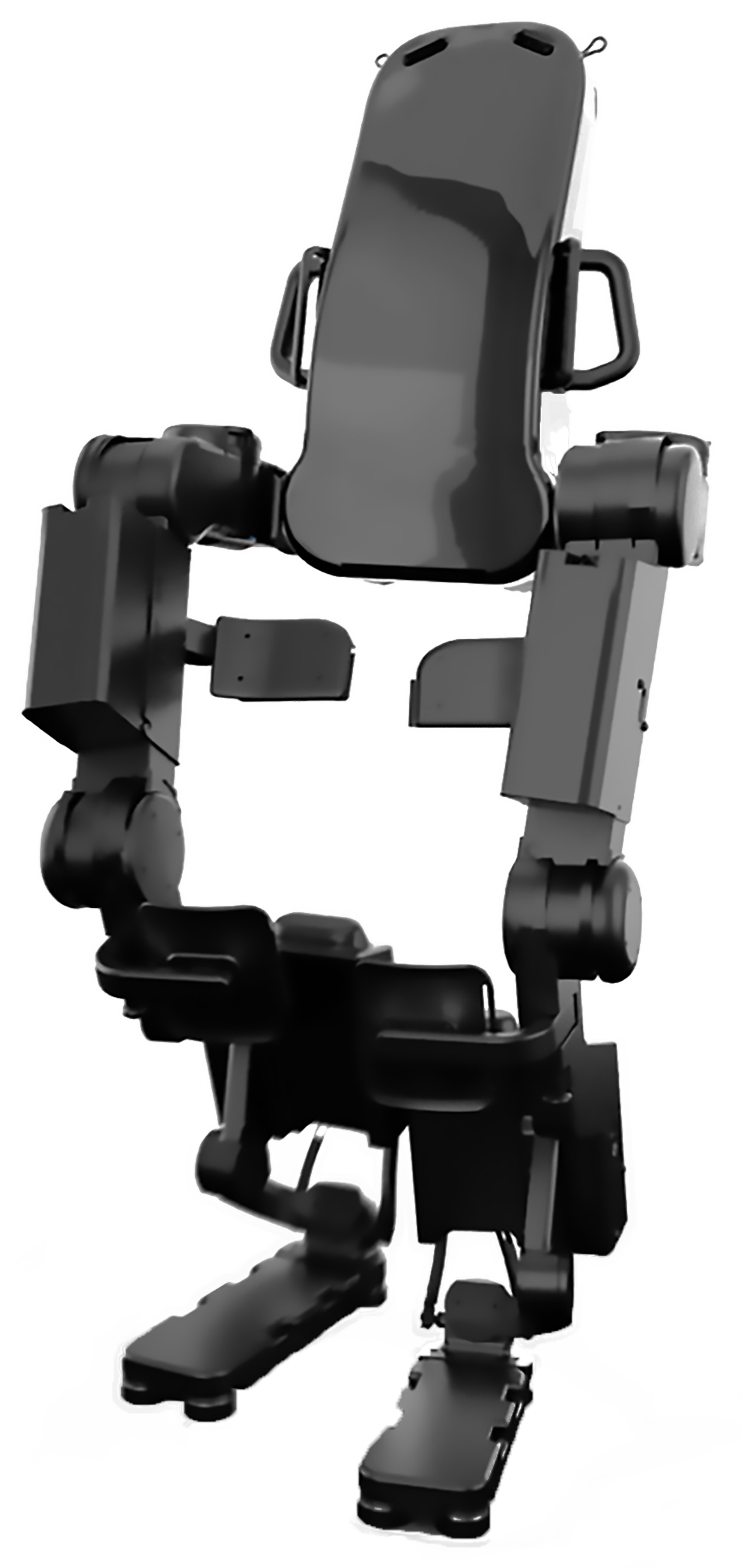
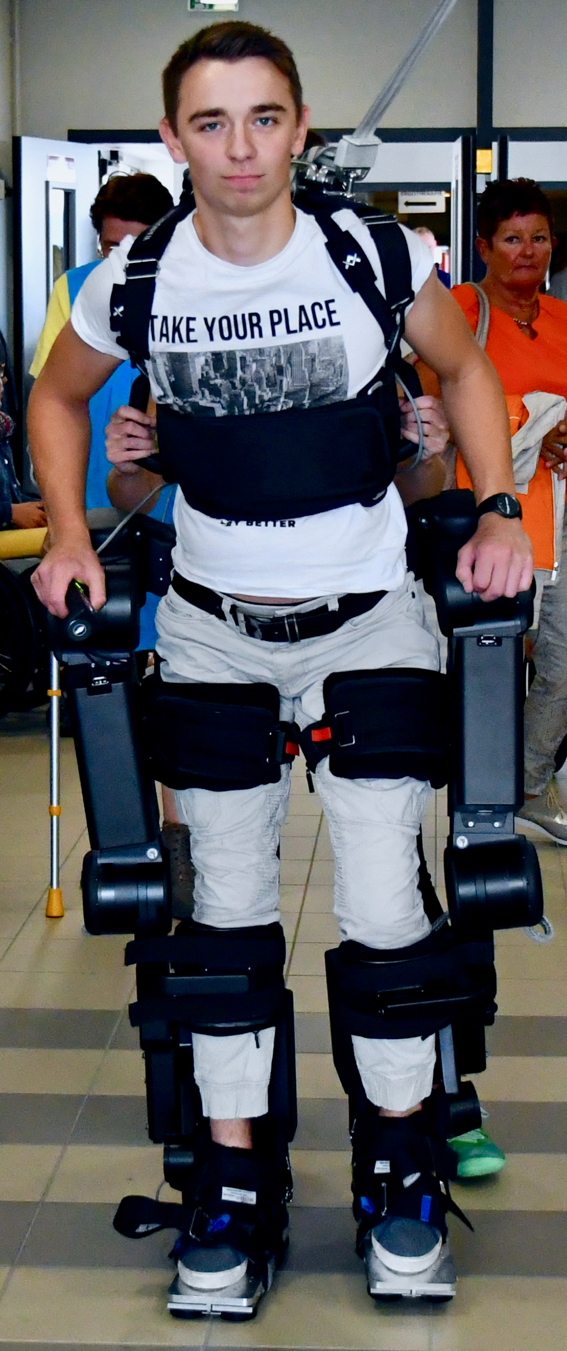
Our method is readily applicable to any complex robotics systems with high-dimensional state for which offline trajectory optimization methods and robust control strategies are already available and efficient. It makes online trajectory planning based on function approximations more accurate and reliable by guaranteeing the feasibility of the predictions, and thereby it is practical for systems where failure is not an option. We demonstrate it on flat-foot walking with the medical exoskeleton Atalante designed by Wandercraft [7].

II RELATED WORK

Even though policy learning may exhibit richer and nicer behaviors than trajectory learning since it performs feedback control, it comes with additional challenges. Indeed, the performance of the few policy learning approaches assessed on real robots were unsatisfactory because of the reality gap [8]. Although major advances were made recently [9], it is not near to be readily available for systems already challenging to control using classic methods. Daumé III suggests to get around this problem by using policy learning to predict trajectories [10]. This can be done by simply passing on earlier predictions as inputs for future predictions. Although trajectories computed in this way can achieve results competitive with trajectory learning [11], it makes policy learning an indirect approach to do trajectory learning, therefore losing its main advantages wrt. trajectory learning.

Both policy and trajectory learning are prone to the so-called distributional shift issue, namely the predictions themselves affect the future states during the execution on the system. Ignoring this leads to very poor performance in the case of policy learning [11, 12, 13]. This is because as soon as the policy makes a mistake, it may encounter completely different observations than those under expert demonstrations, leading to the compounding of errors. The Guided Policy Search (GPS) [4, 14] overcomes this limitation by adapting the states for which expert demonstrations are provided, but also the policy optimization problem itself. Formally, the optimization problem is modified to maximize the actual return of the learned policy, making it less vulnerable to suboptimal experts. The resulting policy is guaranteed to perform well under its induced distribution of states.

The effect of the distributional shift is less dramatic in trajectory learning, since the observations do not take part in the prediction process. Its effect follows directly from the reconstruction error of the function approximation, and thereby requires the latter to fit accurately. Even though trajectory learning using a standard regression may be appropriate in some cases, this does ensure accurate predictions. This approach has proven effective on the bipedal robot Cassie for controlling in real-time the velocity of the center of mass [15, 16], but was unsuccessful in simulation for more complex systems like a human-sized 3D humanoid [4].

Unlike GPS, the policy learning method proposed by Mordatch and Todorov [5] is closely related to trajectory learning since it relies on trajectory optimization to generate expert demonstrations. They seek after a compromise between the optimality of the trajectories and the accuracy of the learned policy, and solves this problem via the Alternating Direction Method of Multipliers. Robustness of the feedback control loop is improved by training the policy to behave as a Linear Quadratic Regular [17]. However, their formulation of the problem does not allow to cancel the reconstruction error out and therefore to get rid of the distributional shift completely. Although this approach is cost-efficient and leads to satisfactory results in simulation for simple systems, it is likely to diverge in practice.

Another aspect to consider is that trajectory optimization based on the direct collocation framework is numerically robust and scalable [18, 19]. It has proven its ability to efficiently solve most trajectory optimization problems, even for complex robotic systems, such as humanoid robots walking trajectory generation [20, 21, 22]. Therefore, adapting the policy learning approaches to trajectory learning appears natural to overcome their respective limitations.

III PRELIMINARIES

III-A Trajectory Optimization Problem

Consider a time-invariant time-continuous dynamical system of the form $\dot{x}(t)=f(x(t),u(t))$, where $x(t)\in\mathbb{R}^{p},\,u(t)\in\mathbb{R}^{q}$ are the state and the controls of the system applied at time $t$, respectively. $f$ denotes the dynamics of the system. Optimization variables minimizing a cost function are highlighted with a superscript asterisk $\cdot^{*}$.

Given a task to perform $\tau\in\mathcal{D}_{\tau}$, where $\mathcal{D}_{\tau}$ is a compact set of $\mathbb{R}^{m}$ denoting the task space, a trajectory optimization problem for such a system can be formulated as

$$(x^{*},u^{*},t^{*})=\underset{(x,u,T)\in\mathcal{C}_{\tau}}{\operatorname*{arg\,min}}\mkern 5.0mu\int_{0}^{T}l(x(t),u(t),T)\,dt,$$ (1)

where $x:t\mapsto x(t),u:t\mapsto u(t)$ are functions whose temporal dependence is implicit, $l$ is the running cost, and $T$ is the duration of the trajectory. $\mathcal{C}_{\tau}$ is the feasibility set

$$\mathcal{C}_{\tau}=\{ (x,u,T)\in\mathcal{D}_{x}\times\mathcal{D}_{u}\times\mathcal{D}_{T}\mid$$

$$c_{T}\left(\tau,x(0),u(0),x(T),u(T),T\right)=0,$$

$$c_{in}(\tau,x(t),u(t),t)\leq 0,$$

$$c_{eq}(\tau,x(t),u(t),t)=0\},$$

where $\mathcal{D}_{x},\mathcal{D}_{u},\mathcal{D}_{T}$ are compact sets embodying the physical limitations of the system. The terminal constraints $c_{T}$ and the inequality and equality constraints $c_{in},c_{eq}$ are continuously differentiable functions that depends on the task $\tau$.

The periodicity and duration of the trajectory are examples of terminal constraints, while the dynamics equation and the admissibility conditions are part of the inequality and equality constraints. A task can be composed of any combination of high-level objectives: for example, for a walking robot, the desired step length and speed.

The state and control functions $x,u$ are further discretized in time sequences of fixed length $L_{T}$. In this context, the optimal trajectory for task $\tau$ is uniquely defined by its sequence of states and duration $(\{x^{*}_{1},x^{*}_{2},\dots,x^{*}_{L_{T}}\},T^{*})$.

III-B Trajectory Learning Problem

The objective is to use the solutions generated through trajectory optimization to train a function approximation parametrized by $W\in\mathbb{R}^{n}$, such that, for any task $\tau$, it outputs a trajectory achieving the task. As the control strategies are not part of the learning process, this can be viewed as a standard regression over a database of $N$ optimal trajectories $\{\tau_{i},(X^{*}_{i}=\{x^{*}_{i,1},x^{*}_{i,2},\dots,x^{*}_{i,L_{T}}\},T^{*}_{i})\}_{i=1}^{N}$, where $N$ must be sufficiently large to span the whole task space.

Formally, training a function approximation consists in finding parameter $W$ giving the best performance in average,

$$W^{*}=\underset{W\in\mathbb{R}^{n}}{\operatorname*{arg\,min}}\mkern 5.0muR_{\gamma}(X^{*},T^{*},W),\\$$ (2)

where $R_{\gamma}(X,T,W)$ is the total reconstruction error, such that

$$R_{\gamma}(X,T,W)\triangleq\!\sum_{i=1}^{N}\left\|X_{i}-\hat{X}(\tau_{i},W))\right\|^{2}\!+\gamma\left\|T_{i}-\hat{T}(\tau_{i},W)\right\|^{2}\!\!,$$ (3)

where $\gamma$ is a weighting factor that determines the trade-off between the state and duration fitting accuracy. The predicted duration and state sequence for a task $\tau$ are denoted $\hat{T}(\tau,W),\hat{X}(\tau,W)$. The subscript $\cdot_{i}$ specifies the task.

It is irrelevant to take into account the constraints of the trajectory optimization problem explicitly in the regression since they are satisfied at the limit when the reconstruction error vanishes. Reducing this error is usually done by increasing number of fitting parameters $n$ to match the regularity of the data. However, it does not bring any guarantee regarding the feasibility of the predictions apart from the training samples, since overfitting may occur. Several techniques exist to alleviate this issue without increasing the computational cost too much, e.g. early stopping and regularization [23, 24, 25], but they do not allow adaptation of the training data. Regularisation of the training data through adaptation may be more computationally demanding, but it ensures reliable predictions by limiting the number of fitting parameters.

IV GUIDED TRAJECTORY LEARNING

We propose to achieve adaptation of the training data by solving simultaneously trajectory optimization and trajectory learning, such that the generated trajectories are perfectly fitted by the function approximation and satisfy the constraints of the original trajectory optimization problem concurrently.

IV-A Consensus Optimization Problem

This problem consists of jointly optimizing a collection of $N$ trajectories achieving a set of tasks $\{\tau_{i}\}_{i\leq N}$, and the parameters of the function approximation $W$ that is intended to fit them. This can be written as follows

$$(X^{*},U^{*},T^{*},W^{*})\,=\mkern-15.0mu\underset{\begin{subarray}{c}(X_{i},U_{i},T_{i})_{1\leq i\leq N}\,\in\,\prod_{i=1}^{N}\mathcal{C}_{\tau_{i}}\\[1.00006pt] W\in\mathbb{R}^{n}\end{subarray}}{\operatorname*{arg\,min}}\mkern 3.0mu\frac{1}{N}\sum_{i=1}^{N}L(X_{i},U_{i},T_{i})$$ (4)

$$\text{st. }X_{i}=\hat{X}(\tau_{i},W),T_{i}=\hat{T}(\tau_{i},W),\,\forall i\in\{0,1,\dots,N\},\vspace{-0.3em}$$

where the tasks $\{\tau_{i}\}_{i\leq N}$ are uniformly sampled, $L(X_{i},U_{i},T_{i})$ is the discretization of the total optimization cost (1)

$$L(X_{i},U_{i},T_{i})\triangleq\frac{T_{i}}{L_{T}}\sum_{t=1}^{L_{T}}l(x_{i,t},u_{i,t},T_{i}).$$

The reconstruction constraint guarantees that the trajectories are perfectly fitted by the function approximation, despite its potentially limited expressive power, and have properties compliant with it. However, solving this problem directly is intractable since it requires to compute the gradient of every trajectory optimization sub-problems at every step of the solver. Indeed, the number of sub-problems $N$ usually ranges from thousands to hundreds of thousands.

IV-B Alternating Direction Method of Multipliers

ADMM [6] is a method to efficiently solve optimization problems composed of a collection of subproblems linked by a single linear equality constraint but otherwise independent, each of them having a readily available solving method. Let’s consider the following separable nonconvex consensus problem [26, 27]

$$(Y^{*},Z^{*})=\mkern-15.0mu\underset{\begin{subarray}{c}(y_{i})_{1\leq i\leq N}\,\in\,\prod_{i=1}^{N}\mathcal{Y}_{i}\\[1.99997pt] Z\in\mathcal{Z}\end{subarray}}{\operatorname*{arg\,min}}\mkern 5.0mu\sum_{i=1}^{N}f_{i}(y_{i})+g(Z)$$ (5)

st.

$$\mathcal{Z}=\left\{Z\in\mathcal{D}_{z}\mid\theta(Z)=0,~{}\sigma(Z)\leq 0\right\}$$

$$Y-Z=0,$$

where $\mathcal{D}_{y}\subset\mathbb{R}^{p},\mathcal{D}_{z}\subset\mathbb{R}^{Np}$ are compact sets. The cost functions $f_{i}:\mathbb{R}^{p}\to\mathbb{R},g:\mathbb{R}^{Np}\to\mathbb{R}$ and the equality and inequality constraints $\psi_{i},\phi_{i},\theta,\sigma$ are twice continuously differentiable.

Such nonconvex problems can be handled efficiently by the Augmented Lagrangian Method [28, 29]. In this case, the augmented Lagrangian in scaled form can be stated as

$$L_{\rho}(Y,Z,\Lambda)\triangleq\sum_{i=1}^{N}f_{i}(y_{i})+g(Z)+\frac{\rho}{2}\left\|Y-Z+\Lambda\right\|^{2}.$$

This is an exact penalty method [30, 31]. In this regard, the original problem can be solved by minimizing it. This can be done in an alternating Gauss-Seidel manner, optimizing each variable while holding the others fixed [6, 32]. This yields Algorithm 1 taken from [26, 27]. $\alpha$ and $\rho^{k}$ are referred to as the dual step size and penalty factor, respectively.

IV-C Guided Trajectory Learning

Let us introduce an additional optimization variable $Z$ in Problem (4), such that $Z_{i}\triangleq(\hat{X}(\tau_{i},W),\gamma\hat{T}(\tau_{i},W))$, where $(\cdot,\cdot)$ stands for the vector concatenation operator.

1 initialization;

while stopping criterion not met do

       for $i\in\{1,...,N\}$ do

            

$$=\underset{y_{i}\in\mathcal{Y}_{i}}{\operatorname*{arg\,min}}\mkern 5.0muf_{i}(y_{i})+\frac{\rho^{k}}{2}\left\|y_{i}-z_{i}^{k}+\lambda^{k}_{i}\right\|^{2}$$ 2

       end for

      

$$=\underset{Z\in\mathcal{Z}}{\operatorname*{arg\,min}}\mkern 5.0mug(Z)+\frac{\rho^{k}}{2}\left\|Y^{k+1}-Z+\Lambda^{k}\right\|^{2}$$ 3

$$=\Lambda^{k}+\alpha(Y^{k+1}-Z^{k+1})$$ 4

end while

Algorithm 1 ADMM for Nonconvex Consensus Problem

The reconstruction constraints becomes

$$(X_{i},\gamma T_{i})-Z_{i}=0$$

$$\text{st. }Z_{i}\in\mathcal{Z}_{\gamma}=\{z\mid\underset{W}{\inf}\mkern 5.0mu\left\|z-(\hat{X}(\tau_{i},W),\gamma\hat{T}(\tau_{i},W))\right\|^{2}=0\}.$$

Then, ADMM can be applied to solve Problem (4). The

Augmented Lagrangian is given by

$$L_{\rho}(X,U,T,Z,\Lambda)=\frac{1}{N}\!\sum_{i=1}^{N}L(X_{i},U_{i},T_{i})+\frac{\rho}{2}\left\|(X,\gamma T)-Z+\Lambda\right\|^{2}\vspace{-0.2em}\!\!\!,$$

where $\Lambda=(\Lambda_{X},\gamma\Lambda_{T})$.

The update rule for step 2 of Algorithm (1) corresponds to

$$(X_{i}^{k+1},\,U_{i}^{k+1},\,T_{i}^{k+1})=\\ \underset{(X_{i},U_{i},T_{i})\in\mathcal{C}_{\tau_{i}}}{\operatorname*{arg\,min}}L(X_{i},U_{i},T_{i})+\frac{\rho^{k}}{2}\left\|(X_{i},\gamma T_{i})-Z_{i}^{k}+\lambda_{i}^{k}\right\|^{2}\!\!,$$ (6)

while the update rule for step 3 is

$$\begin{gathered}Z_{i}^{k+1}=(\hat{X}(\tau_{i},W^{k+1}),\gamma\hat{T}(\tau_{i},W^{k+1}))\\[1.99997pt] \text{st. }W^{k+1}=\underset{W\in\mathbb{R}^{n}}{\operatorname*{arg\,min}}\mkern 5.0muR_{\gamma}(X^{k}+\Lambda_{X},T^{k}+\Lambda_{T},W).\end{gathered}$$ (7)

One can think of the multipliers $\Lambda$ being the cumulative residual prediction error for each task $\tau_{i}$. They reveal where the function approximation makes repeating prediction errors for each trajectory. They modify the regression and trajectory optimization objective functions to give more weight to regions where errors are consistently made. Over iterations, the trajectories become easier to mimic for the function approximation and less optimal wrt. the original objective function, until a consensus is found. This algorithm reduces Problem (4) to a sequence of trajectory optimization and regression problems, each of which is well-studied with efficient solving method. The complete algorithm is summarized in Algorithm 2. A suitable stopping criterion is $\left\|\Lambda^{k+1}-\Lambda^{k}\right\|\leq\epsilon$, where $\epsilon$ depends on the need of accuracy.

IV-D Convergence Analysis

Originally, ADMM was intended to solve convex unconstrained optimization problems, but it has been proven to converge for nonconvex consensus problems [33, 26, 34, 35].

1 generate N tasks uniformly sampled, $\{\tau_{i}\}_{i=1}^{N}\sim U(\mathcal{D}_{\tau})$

2 initialize $(X^{0},U^{0},T^{0})$ by solving the original trajectory optimization problem for each task in parallel using (1)

initialize $\Lambda^{0}$ to zero

update $W^{0}$ using the standard regression (2), deduce $Z^{0}$

3 while not converged do

       update $(X^{k+1},U^{k+1},T^{k+1})$ by solving the modified trajectory optimization problem in parallel using (6)

       update $W^{k+1}$ and deduce $Z^{k+1}$ using (7)

      [0.23em] update $\Lambda^{k+1}$: $\Lambda^{k+1}=\Lambda^{k}+\alpha\left((X^{k+1},\gamma T^{k+1})-Z^{k+1}\right)$

      [0.2em]

end while

Algorithm 2 Guided Trajectory Learning

Proposition 1

Algorithm 1 converges to the closest stationary point to $Z^{0}$, corresponding to a local or global minimum of Problem (5), under these assumptions [26]:

• The consensus optimization problem (5) is feasible.

• $\forall k\in\mathbb{N}$, $y^{k}_{i}$ (resp. $Z^{k}$) computed at step 2 (resp. step 3) of the algorithm is locally or globally optimal.

• Let $\mathcal{L}$ denote the set of limit points of the sequence $\{(Y^{k},Z^{k})\}_{k\in\mathbb{N}}$ and let $(Y^{*},Z^{*})\in\mathcal{L}$. $(Y^{*},Z^{*})$ is a regular point, i.e the gradient vectors at $y_{i}^{*}$ (resp. $Z^{*}$) of the set of active constraints of $\mathcal{Y}_{i}$ (resp. $\mathcal{Z}$) are linearly independent.

• Let define $L$ such that $\forall y_{i}\in\mathcal{D}_{y},\forall Z\in\mathcal{D}_{z}$, $f_{i}$ and $g_{i}$ have a $L$-Lipschitz continuous gradient. The sequence $\{\rho^{k}\}_{k\in\mathbb{N}}$ is increasing and either:

  • $0<\alpha\leq 1$ and $\exists k_{0}\in\mathbb{N}$ st. $\forall k\geq k_{0},\;\rho^{k}>L$.

  • $\alpha=0$ and $\{\rho^{k}\}_{k\in\mathbb{N}}\longrightarrow+\infty$.

It is worth noting that updating the penalty factor $\rho^{k}$ at each iteration is unnecessary for $0<\alpha\leq 1$, as one can keep it equal any value satisfying the converge assumptions. Andreani has proven that, under the additional assumptions, it converges R-linearly for $\alpha$ small enough and $\rho$ constant [27]. Strictly increasing $\rho^{k}$ makes the converge faster (superlinearly in some cases), but it is impracticable at some point. Indeed, high penalty factor leads to ill-conditioning, making the optimization impossible to solve numerically.

Proposition 1 shows that the GTL algorithm can be simplified by setting the dual step size $\alpha$ to 0, which is denoted GTL-0 in the following. It is only guarantee to converge for sequences of penalty factor going to infinity. Otherwise, the price to pay is a non-vanishing reconstruction error. GTL-0 reduces GTL to an instance of the Alternating Direction Penality Method [26] since the multipliers are kept equal to zero. This problem can also be viewed as replacing the reconstruction constraints $X_{i}=\hat{X}(\tau_{i},W),T_{i}=\hat{T}(\tau_{i},W),\,\forall i\in\{0,1,\dots,N\}$ in Problem (4) by the penalized reconstruction cost $\rho^{k}R(X,T,W)$ and solving it in an alternating Gauss-Seidel manner.

IV-E Deconvolution Neural Network as Function Approximation

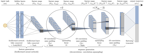
We propose to use a deconvolution neural network [36, 37] as function approximation since it is especially well-suited to generating multi-dimensional temporal sequences [38]. The architecture is described in Fig 2. It combines 1D convolution and upsampling to perform the deconvolution operations, as opposed to the usual transpose convolution that is sensitive to artefacts [39].

Figure 2: Architecture of the neural network used for learning state sequences. A feedforward network generates low dimensional features and a deconvolution network produces sequences from them. The hyperparameters of the feedforward network are the number of hidden layers $N_{h}$ and their size $L_{h}$. The ones of the deconvolution network are the number of upsampling steps $N_{up}$ and the length of the 1D convolution kernel $N_{k}$. The number of channels $N_{ch}$ and the initial length of the features $L_{seq}$ directly derive from them, $N_{ch}\triangleq p\;2^{N_{up}-2},~{}L_{seq}\triangleq\text{ceil}(L_{T}/2^{N_{up}})$. $i$ denotes the index of the upsampling layer.

V EXPERIMENTAL EVALUATION

V-A Experimental Setup

The Medical Exoskeleton Atalante

It is a crutch-less exoskeleton for people with lower limb disabilities. It is an autonomous device, self-balancing and self-supporting. It has 6 actuated revolute joints on each leg,

• 3 joints for the spherical rotation of the hip,

• 1 joint for the flexion of the knee,

• 2 joints for the hinge motion of the ankle.

It features dimensional adjustments for the thigh and tibia lengths to fit the morphology of the patient.

Modeling of the Coupled System Patient-Exoskeleton

The patient is assumed to be rigidly fastened, thus his mass distribution can be aggregated to the one of the exoskeleton. With this in mind, the system exoskeleton-patient is just a specific type of bipedal robot whose kinematics and dynamics properties are patient-specific.

How Trajectories are Generated

The state sequences must guarantee the periodicity of the gait, accurate impact handling, and stability of the exoskeleton. The optimization problem and how to solve it via the Direct Collocation framework is explained thoroughly in [20, 22, 40].

Figure 3: Original trajectories of the ankle joints for uniformly sample tasks.

V-B Training

Learning task

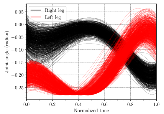
The objective is to learn flat foot walking trajectories for the exoskeleton Atalante. Fig 3 reveals their temporal smoothness, supporting the use of the aforementioned deconvolutional network as the natural way to do it. The system is fully-actuated, thereby the state only comprises the positions and velocities of the 12 actuated joints.

Standard regression is compared to GTL-0 (cf. last part of Section IV-D) instead of GTL for practical reasons. It halves the required storage space wrt. GTL, but most importantly, it enables to update the sample tasks at each iteration of the algorithm instead of keeping the same set all along. It makes parallelization trivial to implement on clusters, and it reduces overfitting that may occur when the number of sample tasks $N$ is relatively limited. Moreover, its performance can only be worse than GTL, giving a lower bound on the expected performance of GTL. The values of the parameters are summarized in Table Ic. The task space $\mathcal{D}_{\tau}$ encompasses,

• the morphology of the patient: height and weight,

• the settings of the exoskeleton: thigh and shank lengths,

• some high-level features of the gait: step length and total duration, among many others (12 in total).

TABLE I: Parameters summary

$m$	$p$	$q$	$L_{T}$
16	24	12	200

(a) learning problem

$N_{h}$	$L_{h}$	$N_{up}$
1	200	5

(b) neural network

$N$	$\gamma$	$\rho^{k}$	$\alpha$
70000	1.0	5.0	0.0

(c) GTL

Validation criteria

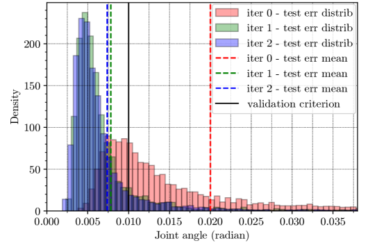
The controllers of the exoskeletons are tuned in such a way that the maximum tracking error of the joint positions can reach up to 0.01 rad in the nominal case, which is accurate enough to achieve stable walking. Thus, we assume that a predicted trajectory is stable on the real robot if the maximum absolute difference between a predicted trajectory and the optimal one is not significantly larger than 0.01rad, referred to as norm-inf error in the following.

Guided Trajectory Learning

We refer to the initialisation of GTL-0 ‘iter 0’ as Regression since it corresponds to the standard regression method, and we compare it to GTL-0 after convergence at ‘iter 2’. Their respective accuracy is summarized in Table II. Unlike Regression, the GTL-0 algorithm shows promising results despite the lack of multipliers. Fig 5 shows that, contrary to GTL-0, the error distribution of Regression is very spread and has a long right tail that never really goes to zero. Therefore, a large part of its predictions has a reconstruction error much larger than the maximum acceptable error of 0.01 rad. Nonetheless, the reconstruction error of GTL-0 does not vanish. This is expected since the residual error is typically handled by the multipliers. It is possible to reduce it further if necessary by increasing the penalty factor $\rho$, at a cost of lowering the conditioning of the optimization problem.

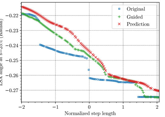
The efficiency of GTL-0 can be understood in the light of Fig 4. It reveals several discontinuities for the solutions to the original problem, which are impossible to fit accurately using a continuous function approximation. By contrast, the trajectories generated via GTL-0 are perfectly continuous wrt. the task. Only one iteration of GTL is sufficient the continuity of the solutions, thereby explaining the very fast convergence of the algorithm in only 2 iterations.

TABLE II: Testing accuracy in norm-inf

Algorithm	Mean (rad)	Mode (rad)	$>0.01$ rad	$>0.015$ rad
Regression	$2.01\times 10^{-2}$	$8.16\times 10^{-3}$	$50.3\%$	$16.1\%$
GTL-0	$7.43\times 10^{-3}$	$4.25\times 10^{-3}$	$10.5\%$	$4.46\%$

Figure 4: Continuity of the trajectories wrt. the task. It shows the effect of the variation of the step length of the walking gait on the angle of the left ankle joint at 20% of the step (see Fig 3). ‘Original’ denotes the solutions of the original trajectory optimization problem for energy minimization cost. ‘Guided’ and ‘Prediction’ correspond to solutions and predictions of GTL-0.

Figure 5: Norm-inf test error distribution over iterations of GTL-0.

V-C Validation in reality on able-bodied people

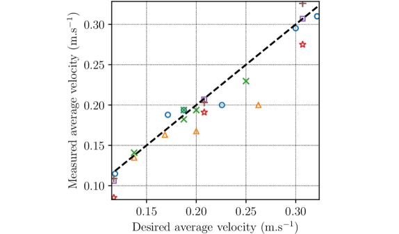
We have evaluated our ability to control the average velocity of the exoskeleton. The desired average velocity is determined by the combination of desired step length and duration. Note that data are only available for GTL-0, since most predictions were unstable on the real robot using the standard regression. In the case of GTL-0, the vast majority of them were stable, and restricting the ranges of the desired step length and duration to 90% during inference lead to stable gaits only. Fig 6 shows that the measured velocities are close to the desired ones for every patient.

Figure 6: From simulation to reality. Comparison between the desired and achieved average velocity on 6 valid people with a different morphology. Each pair marker-color corresponds to one patient.

VI CONCLUSION AND FUTURE WORK

In this work, we present a novel algorithm called GTL that learns a function approximation of the solutions to a trajectory optimization problem over a task space. Accurate and reliable predictions are ensured by simultaneously training the function approximation and adapting the trajectory optimization problem such that its solutions can be perfectly fitted by the function approximation and satisfy the constraints concurrently. It results in a consensus optimization problem that we solve iteratively via ADMM. We demonstrate its efficiency on flat-foot walking with the exoskeleton Atalante.

We believe that our method offers a new scope of applications, such as reinforcement learning, perturbation recovery, or path replanning. Enabling adaption of the architecture of the neural network itself to further improve its efficiency and usability is an exciting direction for future work.

References

- [1] A. Hereid, S. Kolathaya, and A. D. Ames, “Online optimal gait generation for bipedal walking robots using legendre pseudospectral optimization,” in 2016 55th IEEE International Conference on Decision and Control (CDC). IEEE, 2016, pp. 6173–6179.
- [2] T. De Boer, “Foot placement in robotic bipedal locomotion,” Ph.D. dissertation, Delft University of Technology, Netherlands, 2012.
- [3] S. Kajita et al., “Biped walking pattern generation by using preview control of zero-moment point,” in 2003 IEEE International Conference on Robotics and Automation (ICRA), vol. 2. IEEE, 2003, pp. 1620–1626.
- [4] S. Levine and V. Koltun, “Guided policy search,” in 2013 30th International Conference on Machine Learning (ICML), 2013.
- [5] I. Mordatch and E. Todorov, “Combining the benefits of function approximation and trajectory optimization,” in Robotics: Science and Systems, vol. 4, 2014.
- [6] S. Boyd, N. Parikh, E. Chu, B. Peleato, J. Eckstein et al., “Distributed optimization and statistical learning via the alternating direction method of multipliers,” Foundations and Trends in Machine Learning, vol. 3, no. 1, pp. 1–122, 2011.
- [7] “Official Wandercraft’s webplatform,” https://www.wandercraft.eu/en/, Wandercraft, 2012.
- [8] R. T. Hays and M. J. Singer, Simulation fidelity in training system design: Bridging the gap between reality and training. Springer Science & Business Media, 2012.
- [9] K. Bousmalis, A. Irpan, P. Wohlhart, Y. Bai, M. Kelcey, M. Kalakrishnan, L. Downs, J. Ibarz, P. Pastor, K. Konolige et al., “Using simulation and domain adaptation to improve efficiency of deep robotic grasping,” in 2018 IEEE International Conference on Robotics and Automation (ICRA). IEEE, 2018, pp. 4243–4250.
- [10] H. Daumé III, J. Langford, and D. Marcu, “Search-based structured prediction,” Machine Learning, 2009.
- [11] S. Ross, G. J. Gordon, and J. A. Bagnell, “A reduction of imitation learning and structured prediction to no-regret online learning,” The Journal of Thoracic and Cardiovascular Surgery, vol. 147, no. 5, pp. 1488–1492, 2010.
- [12] J. A. Bagnell and S. Ross, “Efficient reductions for imitation learning,” in 2010 30th International Conference on Artificial Intelligence and Statistics (AIStat), 2010.
- [13] J. T. Abbeel and Pieter, “On a connection between importance sampling and the likelihood ratio policy gradient,” 2016 29th Neural Information Processing Systems Conference (NeurIPS), 2016.
- [14] S. Levine and V. Koltun, “Variational policy search via trajectory optimization,” 2013 26th Neural Information Processing Systems Conference (NeurIPS), pp. 207–215, 2013.
- [15] X. Da and J. Grizzle, “Combining trajectory optimization, supervised machine learning, and model structure for mitigating the curse of dimensionality in the control of bipedal robots,” The International Journal of Robotics Research, vol. 38, no. 9, pp. 1063–1097, 2019.
- [16] Z. Xie, G. Berseth, P. Clary, J. Hurst, and M. van de Panne, “Feedback control for cassie with deep reinforcement learning,” 2018 IEEE International Conference on Intelligent Robots and Systems (ICRA), pp. 1241–1246, 2018.
- [17] H. Kwakernaak and R. Sivan, Linear optimal control systems. Wiley-interscience New York, 1972, vol. 1.
- [18] M. Kelly, “An introduction to trajectory optimization: How to do your own direct collocation,” SIAM Review, vol. 59, no. 4, pp. 849–904, 2017.
- [19] C. R. Hargraves and S. W. Paris, “Direct trajectory optimization using nonlinear programming and collocation,” Journal of Guidance, Control, and Dynamics, vol. 10, no. 4, pp. 338–342, 1987.
- [20] A. Hereid, E. A. Cousineau, C. M. Hubicki, and A. D. Ames, “3D dynamic walking with underactuated humanoid robots: A direct collocation framework for optimizing hybrid zero dynamics,” in 2016 IEEE International Conference on Robotics and Automation (ICRA). IEEE, 2016.
- [21] A. Hereid and A. D. Ames, “Frost: Fast robot optimization and simulation toolkit,” in 2017 30th IEEE/RSJ International Conference on Intelligent Robots and Systems (IROS). IEEE, 2017, pp. 719–726.
- [22] J. Grizzle, A. Duburcq, O. Harib, S. Finet, G. Boeris, T. Gurriet, A. D. Ames, M. Masselin, and A. Hereid, “Towards restoring locomotion for paraplegics: Realizing dynamically stable walking on exoskeletons,” in 2018 IEEE International Conference on Robotics and Automation (ICRA). IEEE, 2018, pp. 2804–2811.
- [23] F. Girosi, M. Jones, and T. Poggio, “Regularization theory and neural networks architectures,” Neural computation, vol. 7, no. 2, pp. 219–269, 1995.
- [24] N. Srivastava, G. Hinton, A. Krizhevsky, I. Sutskever, and R. Salakhutdinov, “Dropout: a simple way to prevent neural networks from overfitting,” The journal of machine learning research, vol. 15, no. 1, pp. 1929–1958, 2014.
- [25] H. Zou and T. Hastie, “Regularization and variable selection via the elastic net,” Journal of the royal statistical society: series B (statistical methodology), vol. 67, no. 2, pp. 301–320, 2005.
- [26] S. Magnusson, P. C. Weeraddana, M. G. Rabbat, and C. Fischione, “On the convergence of alternating direction lagrangian methods for nonconvex structured optimization problems,” IEEE Transactions on Control of Network Systems, 2016.
- [27] R. Andreani, E. G. Birgin, J. M. Martínez, and M. L. Schuverdt, “On augmented lagrangian methods with general lower-level constraints,” SIAM Journal on Optimization, vol. 18, no. 4, pp. 1286–1309, 2007.
- [28] D. P. Bertsekas, “Multiplier methods: a survey,” Automatica, vol. 12, no. 2, pp. 133–145, 1976.
- [29] ——, Constrained optimization and Lagrange multiplier methods. Academic press, 1982.
- [30] S.-P. Han and O. L. Mangasarian, “Exact penalty functions in nonlinear programming,” Mathematical Programming, vol. 17, no. 1, pp. 251–269, 1979.
- [31] G. Di Pillo and L. Grippo, “Exact penalty functions in constrained optimization,” SIAM Journal on control and optimization, vol. 27, no. 6, pp. 1333–1360, 1989.
- [32] J. C. Bezdek and R. J. Hathaway, “Convergence of alternating optimization,” Neural, Parallel & Scientific Computations, vol. 11, no. 4, pp. 351–368, 2003.
- [33] M. Hong, Z. Q. Luo, and M. Razaviyayn, “Convergence analysis of alternating direction method of multipliers for a family of nonconvex problems,” in 2015 40th IEEE International Conference on Acoustics, Speech and Signal Processing (ICASSP). IEEE, 2015.
- [34] M. Hong and Z.-Q. Luo, “On the linear convergence of the alternating direction method of multipliers,” Mathematical Programming, vol. 162, no. 1-2, pp. 165–199, 2017.
- [35] W. I. Zangwill, Nonlinear programming: a unified approach. Prentice-Hall Englewood Cliffs, NJ, 1969, vol. 196, no. 9.
- [36] Z. Wojna et al., “The devil is in the decoder: Classification, regression and gans,” International Journal of Computer Vision (IJCV), 2019.
- [37] C. Dong, C. C. Loy, K. He, and X. Tang, “Image super-resolution using deep convolutional networks,” IEEE transactions on pattern analysis and machine intelligence, vol. 38, no. 2, pp. 295–307, 2015.
- [38] H. Tachibana, K. Uenoyama, and S. Aihara, “Efficiently trainable text-to-speech system based on deep convolutional networks with guided attention,” in 2018 43th IEEE International Conference on Acoustics, Speech and Signal Processing (ICASSP). IEEE, 2018, pp. 4784–4788.
- [39] A. Odena, V. Dumoulin, and C. Olah, “Deconvolution and checkerboard artifacts,” Distill, 2016.
- [40] A. Hereid, C. M. Hubicki, E. A. Cousineau, and A. D. Ames, “Dynamic humanoid locomotion: A scalable formulation for hzd gait optimization,” IEEE Transactions on Robotics, 2018.