Discriminator-Actor-Critic:
Addressing Sample Inefficiency and Reward Bias in Adversarial Imitation Learning
Abstract
We identify two issues with the family of algorithms based on the Adversarial Imitation Learning framework. The first problem is implicit bias present in the reward functions used in these algorithms. While these biases might work well for some environments, they can also lead to sub-optimal behavior in others. Secondly, even though these algorithms can learn from few expert demonstrations, they require a prohibitively large number of interactions with the environment in order to imitate the expert for many real-world applications. In order to address these issues, we propose a new algorithm called Discriminator-Actor-Critic that uses off-policy Reinforcement Learning to reduce policy-environment interaction sample complexity by an average factor of 10. Furthermore, since our reward function is designed to be unbiased, we can apply our algorithm to many problems without making any task-specific adjustments.
1 Introduction
The Adversarial Imitation Learning (AIL) class of algorithms learns a policy that robustly imitates an expert’s actions via a collection of expert demonstrations, an adversarial discriminator and a reinforcement learning method. For example, the Generative Adversarial Imitation Learning (GAIL) algorithm (Ho & Ermon, 2016) uses a discriminator reward and a policy gradient algorithm to imitate an expert RL policy on standard benchmark tasks. Similarly, the Adversarial Inverse Reinforcement Learning (AIRL) algorithm (Fu et al., 2017) makes use of a modified GAIL discriminator to recover a reward function that can be used to perform Inverse Reinforcement Learning (IRL) (Abbeel & Ng, 2004) and who‘s subsequent dense reward is robust to changes in dynamics or environment properties. Importantly, AIL algorithms such as GAIL and AIRL, obtain higher performance than supervised Behavioral Cloning (BC) when using a small number of expert demonstrations; experimentally suggesting that AIL algorithms alleviate some of the distributional drift (Ross et al., 2011) issues associated with BC. However, both these AIL methods suffer from two important issues that will be addressed by this work: 1) a large number of policy interactions with the learning environment is required for policy convergence and 2) bias in the reward function formulation and improper handling of environment terminal states introduces implicit rewards priors that can either improve or degrade policy performance.
While GAIL requires as little as 200 expert frame transitions (from 4 expert trajectories) to learn a robust reward function on most MuJoCo (Todorov et al., 2012) tasks, the number of policy frame transitions sampled from the environment can be as high as 25 million in order to reach convergence. If PPO (Schulman et al., 2017) is used in place of TRPO (Schulman et al., 2015), the sample complexity can be reduced somewhat (for example, as in Figure 4, 25 million steps reduces to approximately 10 million steps), however it is still intractable for many robotics or real-world applications. In this work we address this issue by incorporating an off-policy RL algorithm (TD3 (Fujimoto et al., 2018)) and an off-policy discriminator to dramatically decrease the sample complexity by many orders of magnitude.
In this work we will also illustrate how the specific form of AIL reward function used has a large impact on agent performance for episodic environments. For instance, as we will show, a strictly positive reward function prevents the agent from solving tasks in a minimal number of steps and a strictly negative reward function is not able to emulate a survival bonus. Therefore, one must have some knowledge of the true environment reward and incorporate such priors to choose a suitable reward function for successful application of GAIL and AIRL. We will discuss these issues in formal detail, and present a simple - yet effective - solution that drastically improves policy performance for episodic environments; we explicitly handle absorbing state transitions by learning the reward associated with these states.
We propose a new algorithm, which we call Discriminator-Actor-Critic (DAC), that is compatible with both the popular GAIL and AIRL frameworks, incorporates explicit terminal state handling, an off-policy discriminator and an off-policy actor-critic reinforcement learning algorithm. DAC achieves state-of-the-art AIL performance for a number of difficult imitation learning tasks. More specifically, in this work we:
-
•
Identify, and propose solutions for the problem of bias in discriminator-based reward estimation in imitation learning.
-
•
Accelerate learning from demonstrations by providing an off-policy variant for AIL algorithms, which significantly reduces the number of agent-environment interactions.
-
•
Illustrate the robustness of DAC to noisy, multi-modal and constrained expert demonstrations, by performing experiments with human demonstrations on non-trivial robotic tasks.

2 Related Work
Imitation learning has been broadly studied under the twin umbrellas of Behavioral Cloning (BC) (Bain & Sommut, 1999; Ross et al., 2011) and Inverse Reinforcement Learning (IRL) (Ng & Russell, 2000). To recover the underlying policy, IRL performs an intermediate step of estimating the reward function followed by RL on this function (Abbeel & Ng, 2004; Ratliff et al., 2006). Operating in the Maximum Entropy IRL formulation (Ziebart et al., 2008), Finn et al. (2016b) introduce an iterative-sampling based estimator for the partition function, deriving an algorithm for recovering non-linear reward functions in high-dimensional state and action spaces. Finn et al. (2016a) and Fu et al. (2017) further extend this by exploring the theory and practical considerations of an adversarial IRL framework, and draw connections between IRL and cost learning in GANs (Goodfellow et al., 2014).
In practical scenarios, we are often interested in recovering the expert’s policy, rather than the reward function. Following Syed et al. (2008), and by treating imitation learning as an occupancy matching problem, Ho & Ermon (2016) proposed a Generative Adversarial Imitation Learning (GAIL) framework for learning a policy from demonstrations, which bypasses the need to recover the expert’s reward function. More recent work extends the framework by improving on stability and robustness (Wang et al., 2017; Kim & Park, 2018) and making connections to model-based imitation learning (Baram et al., 2017). These approaches generally use on-policy algorithms for policy optimization, trading off sample efficiency for training stability.
Learning complex behaviors from sparse reward signals poses a significant challenge in reinforcement learning. In this context, expert demonstrations or template trajectories have been successfully used (Peters & Schaal, 2008) for initalizing RL policies. There has been a growing interest in combining extrinsic sparse reward signals with imitation learning for guided exploration (Zhu et al., 2018; Kang et al., 2018; Le et al., 2018; Vecerík et al., 2017). Off policy learning from demonstration has been previously studied under the umbrella of accelerating reinforcement learning by structured exploration (Nair et al., 2017; Hester et al., 2017) An implicit assumption of these approaches is access to demonstrations and reward from the environment; our approach requires access only to expert demonstrations.
Our work is most related to AIL algorithms (Ho & Ermon, 2016; Fu et al., 2017; Torabi et al., 2018). In contrast to Ho & Ermon (2016) which assumes (state-action-state’) transition tuples, Torabi et al. (2018) has weaker assumptions, by relying only on observations and removing the dependency on actions. The contributions in this work are complementary (and compatible) to Torabi et al. (2018).
3 Background
3.1 Markov Decision Process
We consider problems that satisfy the definition of a Markov Decision Process (MDP), formalized by the tuple: . Here , represent the state and action spaces respectively, is the initial state distribution, defines environment dynamics represented as a conditional state distribution, is reward function and the return discount factor.
In continuing tasks, where environment interactions are unbounded in sequence length, the returns for a trajectory , are defined as . In order to use the same notation for episodic tasks, whose finite length episodes end when reaching a terminal state, we can define a set of absorbing states (Sutton et al., 1998) that an agent enters after the end of episode, has zero reward and transitions to itself for all agent actions: , and (see Figure 2). With this above absorbing state notation, returns can be defined simply as . In reinforcement learning, the goal is to learn a policy that maximizes expected returns.
In many imitation learning and IRL algorithms a common assumption is to assign zero reward value, often implicitly, to absorbing states. As we will discuss in detail in Section 4.2, our DAC algorithm will assign a learned, potentially non-zero reward for absorbing states and we will demonstrate empirically in Section 4.1.1, that it is extremely important to properly handle the absorbing states for algorithms where rewards are learned.
3.2 Adversarial Imitation Learning
In order to learn a robust reward function we use the GAIL framework (Ho & Ermon, 2016). Inspired by maximum entropy IRL (Ziebart et al., 2008) and Generative Adversarial Networks (GANs) (Goodfellow et al., 2014), GAIL trains a binary classifier, , referred to as the discriminator, to distinguish between transitions sampled from an expert and those generated by the trained policy. In standard GAN frameworks, a generator gradient is calculated by backprop through the learned discriminator. However, in GAIL the policy is instead provided a reward for confusing the discriminator, which is then maximized via some on-policy RL optimization scheme (e.g. TRPO (Schulman et al., 2015)):
| (1) |
where is an entropy regularization term.
The rewards learned by GAIL might not correspond to a true reward (Fu et al., 2017) but can be used to match the expert occupancy measure, which is defined as . Ho & Ermon (2016) draw analogies between distribution matching using GANs and occupancy matching with GAIL. They demonstrate that by maximizing the above reward, the algorithm matches occupancy measures of the expert and trained policies with some regulation term defined by the choice of GAN loss function.
In principle, GAIL can be incorporated with any on-policy RL algorithm. However, in this work we adapt it for off-policy training (discussed in Section 4.3). As can be seen from Equation 1, the algorithm requires state-action pairs to be sampled from the learned policy. In Section 4.3 we will discuss what modifications are necessary to adapt the algorithm to off-policy training.
4 Discriminator-Actor-Critic
In this section we will present the Discriminator-Actor-Critic (DAC) algorithm. This algorithm is comprised of two parts: a method for unbiasing adversarial reward functions, discussed in Section 4.2, and an off-policy discriminator formulation of AIL, discussed in Section 4.3. A high level pictorial representation of this algorithm is also shown in Figure 1. The algorithm is formally summarized in Appendix A.
4.1 Bias in Reward Functions
In the following section, we present examples of bias present in reward functions in different AIL algorithms:
-
•
In the GAIL framework, and follow-up methods, such as GMMIL (Kim & Park, 2018) and AIRL, zero reward is implicitly assigned for absorbing states, while some reward function, , assigns rewards for intermediate states depending on properties of a task.
-
•
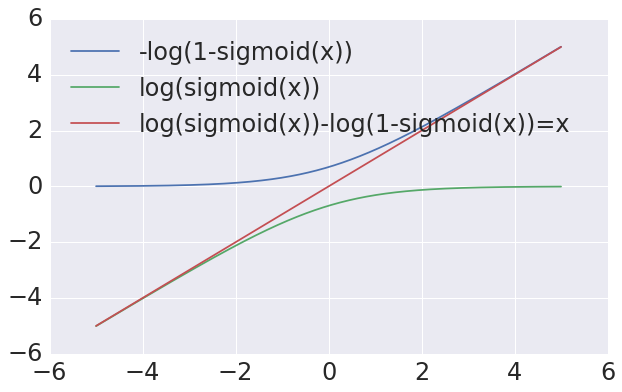
For certain environments, a survival bonus in the form of per-step positive reward is added to the rewards received by the agent. This encourages agents to survive longer in the environment to collect more rewards. We observe that a commonly used form of the reward function: has worked well for environments that require a survival bonus. However, since the recovered reward function can never be negative, it cannot recover the true reward function for environments where an agent is required to solve the task as quickly as possible. Using this form of the reward function will lead to sub-optimal solutions. The agent is now incentivized to move in loops or take small actions (in continuous action spaces) that keep it close to the states in the expert’s trajectories. The agent keeps collecting positive rewards without actually attempting to solve the task demonstrated by the expert (see Section 3).111Note that this behavior was described in the early reward shaping literature (Ng et al., 1999).
-
•
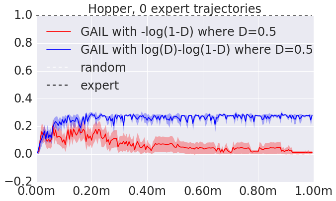
Another reward formulation is . This is often used for tasks with a per step penalty, when a part of a reward function consists of a negative constant assigned unconditionally of states and actions. However, this variant assigns only negative rewards and cannot learn a survival bonus. Such strong priors might lead to good results even with no expert trajectories (as shown in Figure 5).
From an end-user’s perspective, it is undesirable to have to craft a different reward function for every new task. In the next section, we describe an illustrative example of a typical failure of biased reward functions. We also propose a method to unbias the reward function in our imitation learning algorithm such that it is able to recover different reward functions without adjusting the form of reward function.
4.1.1 An Illustrative Example of Reward Bias
Firstly, we illustrate how cannot match the expert trajectories with environments with per-step penalties. Consider a simple MDP with 3 states: , , , where is a goal state and agents receive a reward by reaching the goal state, and 3 actions: ; where is such that , as shown in Figure 3 a). And for every state the expert demonstration is the following: , , (as shown in Figure 3 b), and which clearly reaches the goal state in the optimal number of steps. Now consider the trajectory of Figure 3 c): . This trajectory will have the return . While the expert return is .
Assuming that we have a discriminator trained to convergence, it will assign a value that is close to zero, since it never appears in expert demonstrations. Therefore, from one can derive . Thus, for the loopy trajectory to have a smaller return than our expert policy, we need , if (a standard value). However, the optimal values for GAN discriminator in this case are and . Hence, the inequality above does not hold. As such, the convergence of GAIL to the expert policy with this reward function is possible under only certain values of , and this value depends heavily on the task MDP. At the same time, since the reward function is strictly positive it implicitly provides a survival bonus. In other words, regardless of how the discriminator actually classifies state-action tuples, it always rewards the policy for avoiding absorbing states (see Section 5.2). Fundamentally, this characteristic makes it difficult to attribute policy performance to the robustness of the GAIL learned reward since the RL optimizer can often solve the task as long as the reward is strictly positive.
Another common reward variant, , which corresponds to the original saturating loss for GANs, penalizes every step and leads to collapsing in environments with a survival bonus. This phenomenon can be demonstrated using a reasoning similar to the one stated above.
Finally, AIRL uses the reward function: , which can assign both positive and negative rewards for each time step. In AIRL, as in the original GAIL, the agent receives zero reward at the end of the episode, leading to sub-optimal policies (and training instability) in environments with a survival bonus. In the beginning of training this reward function assigns rewards with a negative bias because it is easy for the discriminator to distinguish samples for an untrained policy and an expert, and so it is common for learned agents to finish an episode earlier (to avoid additional negative penalty) instead of trying to imitate the expert.
4.2 Unbiasing Reward Functions
In order to resolve the issues described in Section 4.1.1, we suggest explicitly learning rewards for absorbing states for expert demonstrations and trajectories produced by a policy. Thus, the returns for final states are defined now with a learned reward instead of just .
We implemented these absorbing states by adding an extra indicator dimension that indicates whether the state is absorbing or not, for absorbing states we set the indicator dimension to one and all other dimensions to zero. The GAIL discriminator can distinguish whether reaching an absorbing state is a desirable behavior from the expert’s perspective and assign the rewards accordingly.
Instead of recursively computing the Q values, this issue can be addressed by analytically deriving the following returns for the terminal states: . However, in practice this alternative was much less stable.
4.3 Addressing Sample Inefficiency
As previously mentioned, GAIL requires a significant number of interactions with a learning environment in order to imitate an expert policy. To address the sample inefficiency of GAIL, we use an off-policy RL algorithm and perform off-policy training of the GAIL discriminator performed in the following way: instead of sampling trajectories from a policy directly, we sample transitions from a replay buffer collected while performing off-policy training:
| (2) |
Equation 2 tries to match the occupancy measures between the expert and the distribution induced by the replay buffer , which can be seen as a mixture of all policy distributions that appeared during training, instead of the latest trained policy . In order to recover the original on-policy expectation, one needs to use importance sampling:
| (3) |
However, it can be challenging to properly estimate these densities and the discriminator updates might have large variance. We found that the algorithm works well in practice with the importance weight omitted.
We use the GAIL discriminator in order to define rewards for training a policy using TD3; we update per-step rewards every time when we pull transitions from the replay buffer using the latest discriminator. The TD3 algorithm provides a good balance between sample complexity and simplicity of implementation and so is a good candidate for practical applications. Additionally, depending on the distribution of expert demonstrations and properties of the task, off-policy RL algorithms can effectively handle multi-modal action distributions; for example, this can be achieved for the Soft Actor Critic algorithm (Haarnoja et al., 2018b) using the reparametrization trick (Kingma & Ba, 2014) with a normalizing flow (Rezende & Mohamed, 2015) as described in Haarnoja et al. (2018a).
5 Experiments
We implemented the DAC algorithm described in Section 4.3 using TensorFlow Eager (Abadi et al., 2015) and we evaluated it on popular benchmarks for continuous control simulated in MuJoCo (Todorov et al., 2012). We also define a new set of robotic continuous control tasks (described in detail below) simulated in PyBullet (Coumans & Bai, 2016), and a Virtual Reality (VR) system for capturing human examples in this environment; human examples constitute a particularly challenging demonstration source due to their noisy, multi-modal and potentially sub-optimal nature, and we define episodic multi-task environments as a challenging setup for adversarial imitation learning.
For the critic and policy networks we used the same architecture as in Fujimoto et al. (2018): a 2 layer MLP with ReLU activations and 400 and 300 hidden units correspondingly. We also add gradient clipping (Pascanu et al., 2013) to the actor network with clipping value of 40. For the discriminator we used the same architecture as in Ho & Ermon (2016): a 2 layer MLP with 100 hidden units and activations. We trained all networks with the Adam optimizer (Kingma & Ba, 2014) and decay learning rate by starting with initial learning rate of and decaying it by 0.5 every training steps for the actor network.
In order to make the algorithm more stable, especially in the off-policy regime when the discriminator can easily over-fit to training data, we use regularization in the form of gradient penalties (Gulrajani et al., 2017) for the discriminator. Originally, this was introduced as an alternative to weight clipping for Wasserstein GANs (Arjovsky et al., 2017), but later it was shown that it helps to make JS-based GANs more stable as well (Lucic et al., 2017).
We replicate the experimental setup of Ho & Ermon (2016): expert trajectories are sub-sampled by retaining every 20 time steps starting with a random offset (and fixed stride). It is worth mentioning that, as in Ho & Ermon (2016), this procedure is done in order to make the imitation learning task harder. With full trajectories, behavioral cloning provides competitive results to GAIL.
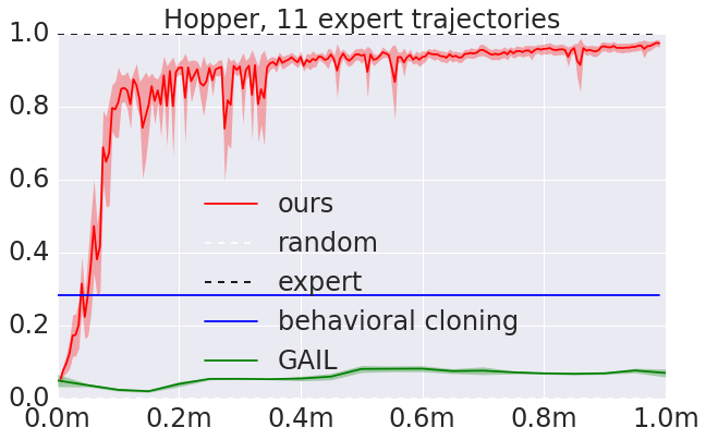
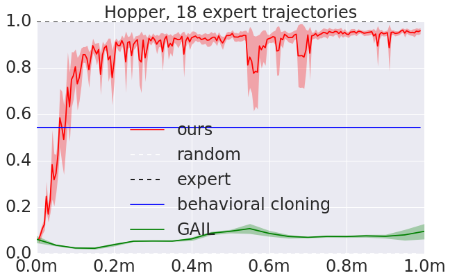
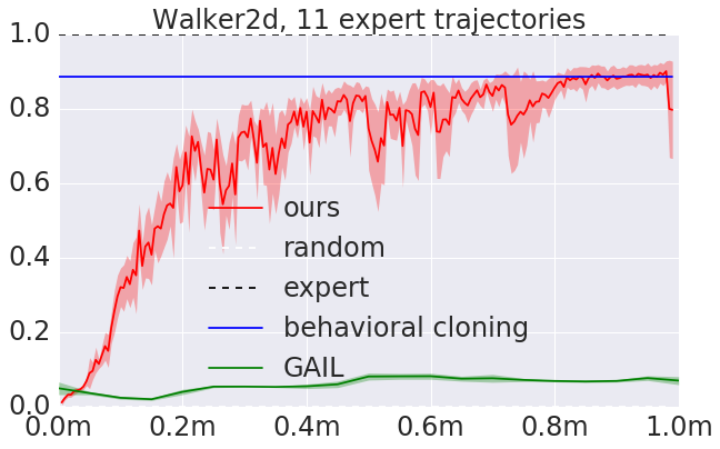
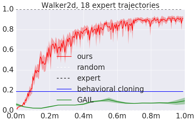
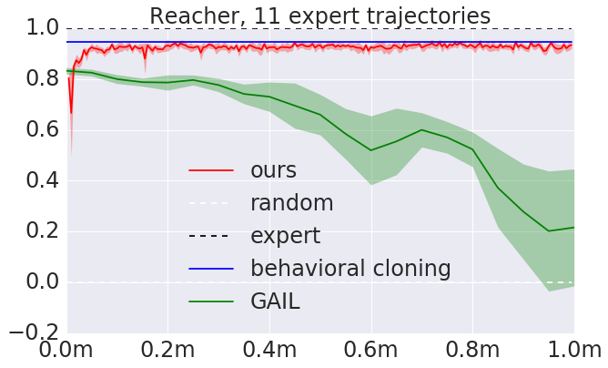
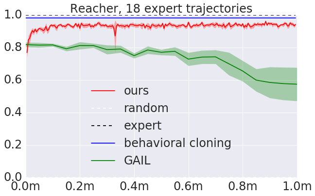
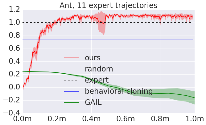
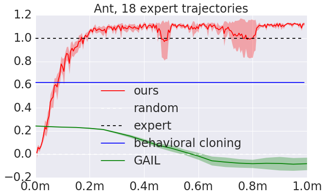
Following Henderson et al. (2017) and Fujimoto et al. (2018), we perform evaluation using 10 different random seeds. For each seed, we compute average episode reward using 10 episodes and running the policy without random noise. As in Ho & Ermon (2016) we plot reward normalized in such a way that zero corresponds to a random reward while one corresponds to expert rewards. We compute mean over all seeds and visualize half standard deviations. In order to produce the same evaluation for GAIL we used the original implementation222https://github.com/openai/imitation of the algorithm.
5.1 Off Policy DAC Algorithm
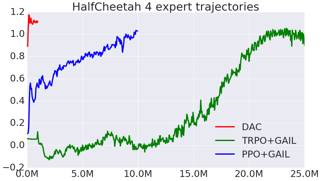
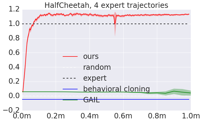
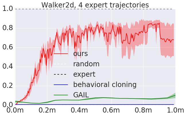
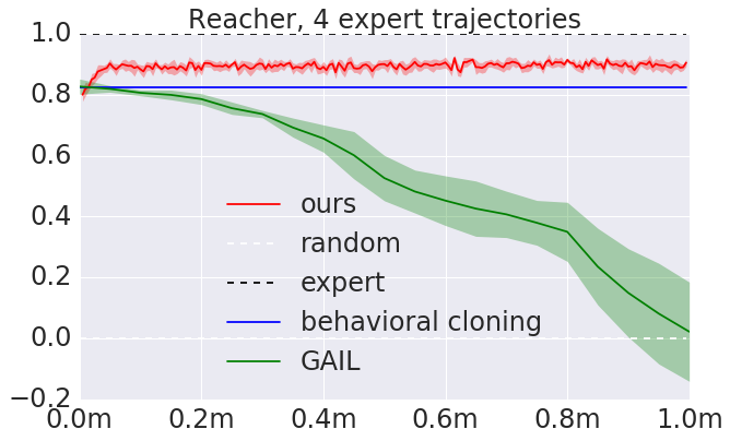
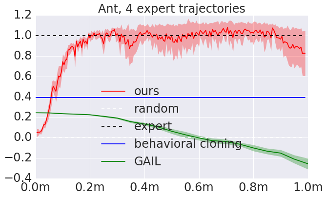
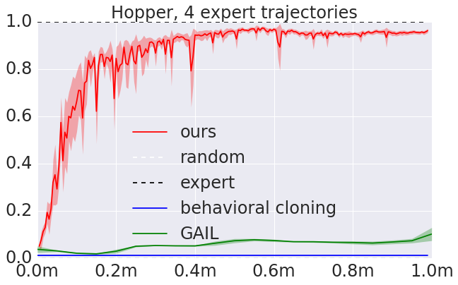
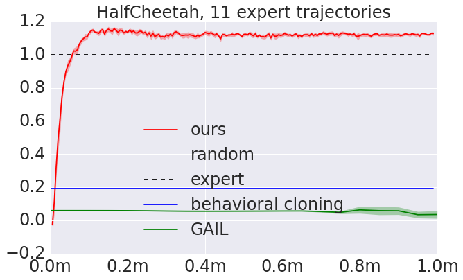
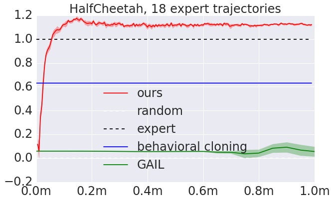
Evaluation results of the DAC algorithm on a suite of MuJoCo tasks are shown in Figure 4, as are the GAIL (TRPO) and BC basline results. In the top-left plot, we show DAC is an order of magnitude more sample efficent than then TRPO and PPO based GAIL baselines. In the other plots, we show that by using a significantly smaller number of environment steps (orders of magnitude fewer), our DAC algorithm reaches comparable expected reward as the GAIL baseline. Furthermore, DAC outperforms the GAIL baseline on all environments within a 1 million step threshold. A comprehensive suit of results can be found in Appendix B, Figure 8.
5.2 Reward Bias
As discussed in Section 4.1.1, the reward function variants used with GAIL can have implicit biases when used without handling absorbing states. Figure 5 demonstrates how bias affects results on an environment with survival bonus when using the reward function of Ho & Ermon (2016): . Surprisingly, when using a fixed and untrained GAIL discriminator that outputs 0.5 for every state-action pair, we were able to reach episode rewards of around 1000 on the Hopper environment, corresponding to approximately one third of the expert performance. Without any reward learning, and using no expert demonstrations, the agent can learn a policy that outperforms behavioral cloning (Figure 5). Therefore, the choice of a specific reward function might already provide strong prior knowledge that helps the RL algorithm to move towards recovering the expert policy, irrespective of the quality of the learned reward.
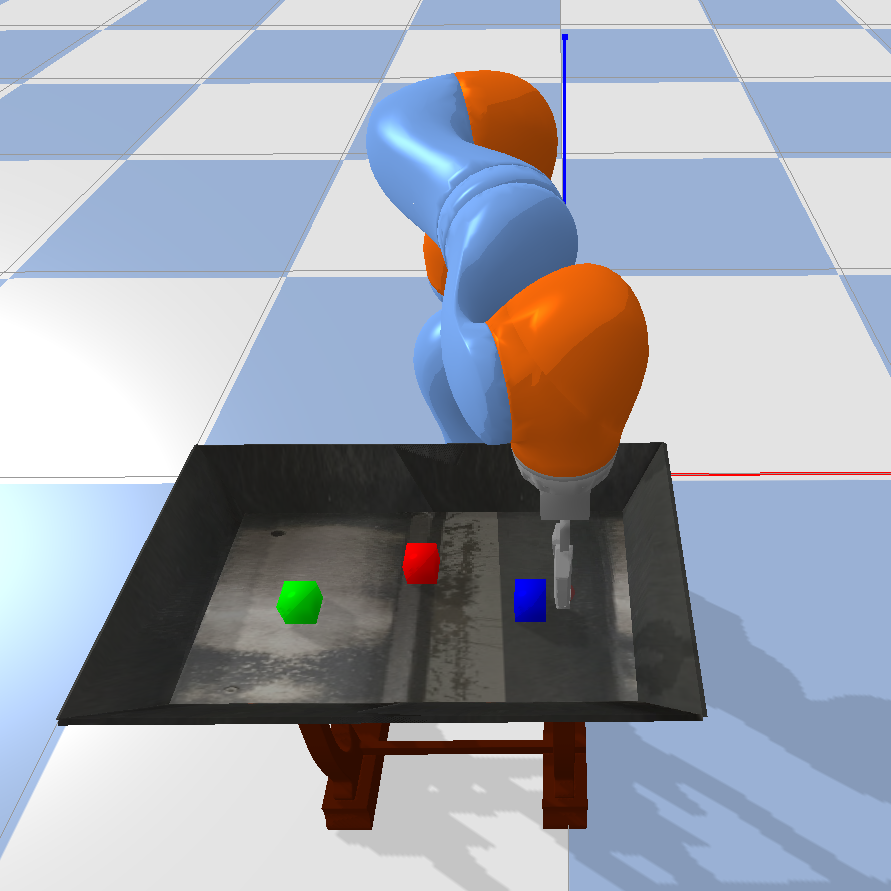
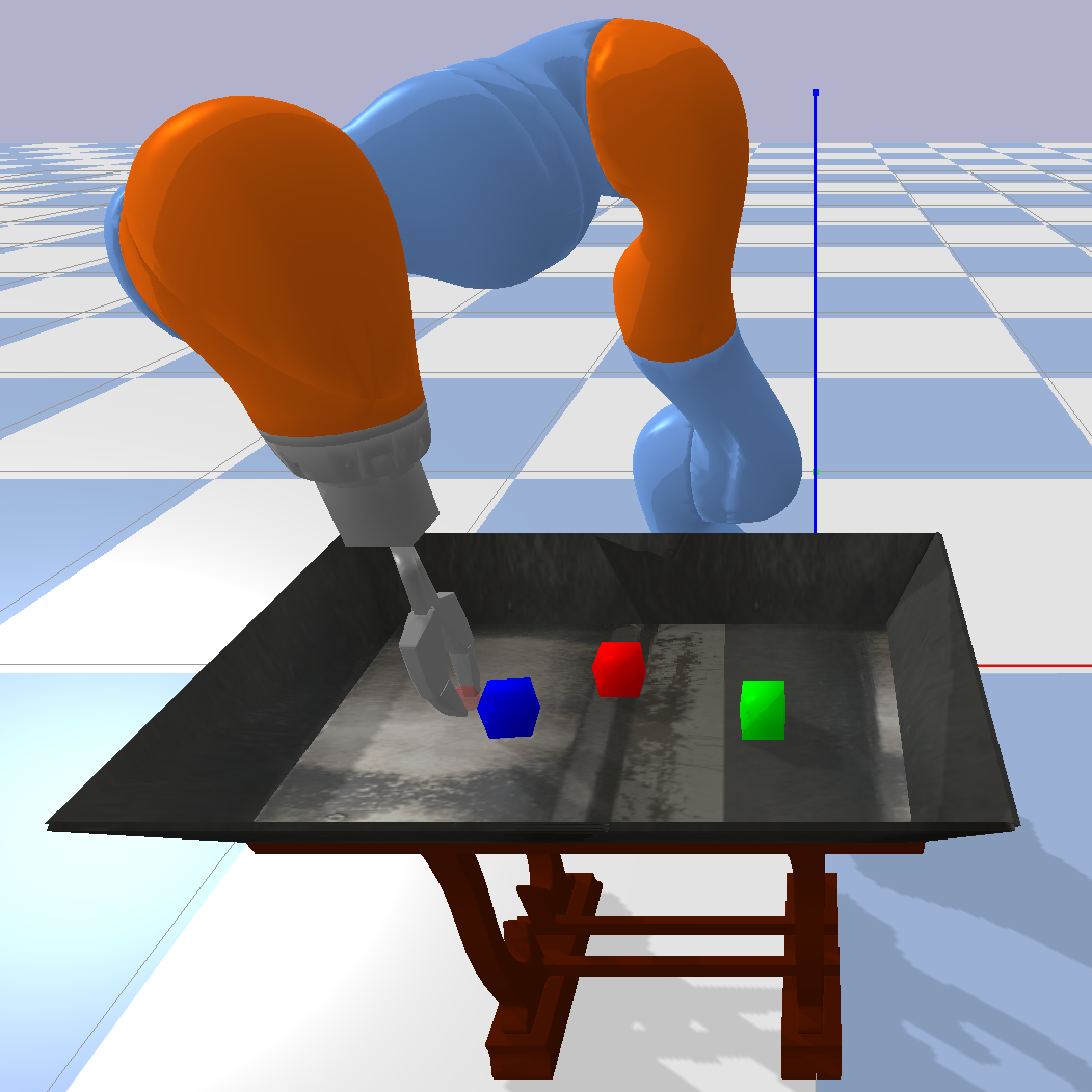
Additionally, we evaluated our method on two environments with per-step penalty (see Figure 6). These environment are simulated in PyBullet and consist of a Kuka IIWA arm and 3 blocks on a virtual table. A rendering of the environment can be found in Appendix C, Figure 9. Using a Cartesian displacement action for the gripper end-effector and a compact observation-space (consisting of each block’s 6DOF pose and the Kuka’s end-effector pose), the agent must either a) reach one of the 3 blocks in the shortest number of frames possible (the target block is provided to the policy as a one-hot vector), which we call Kuka-Reach, or b) push one block along the table so that it is adjacent to another block, which we call Kuka-PushNext. For evaluation, we define a sparse reward indicating successful task completion (within some threshold). For these imitation learning experiments, we use human demonstrations collected with a VR setup, where the participant wears a VR headset and controls in real-time the gripper end-effector using a 6DOF controller.
Using the reward defined as and without absorbing state handling, the agent completely fails to recover the expert policy given expert trajectories without sub-sampling (as shown in Figure 5). In contrast, our DAC algorithm quickly learns to imitate the expert, despite using noisy and potentially sub-optimal human demonstrations.
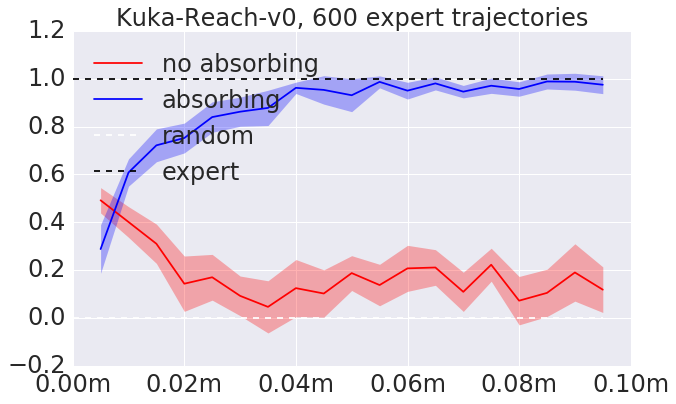
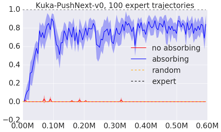
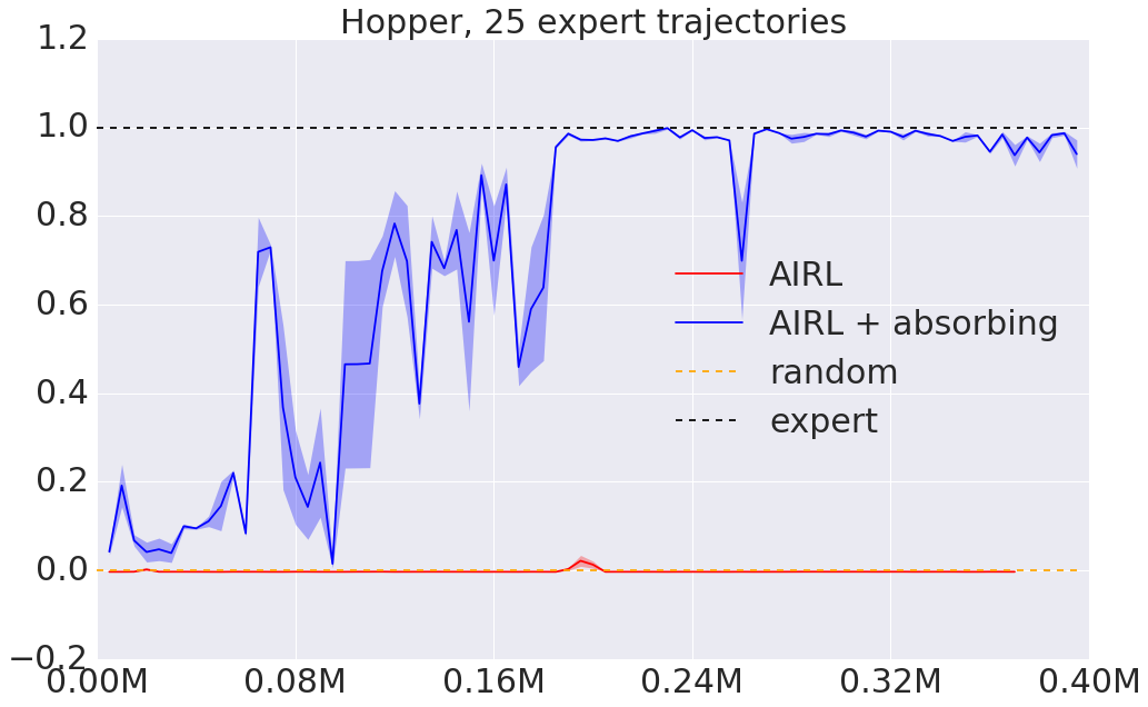
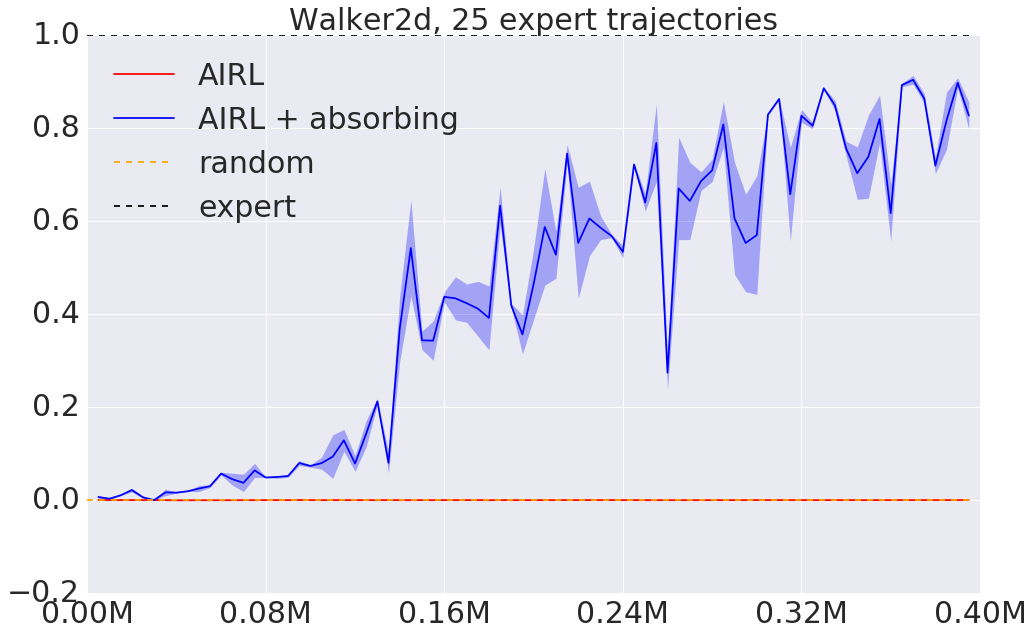
As discussed, alternative reward functions do not have this positive bias but still require proper handling of the absorbing states as well in order to avoid early termination due to incorrectly assigned per-frame penalty. Figure 7 illustrates results for AIRL with and without learning rewards for absorbing states. For these experiments we use the discriminator structure from Fu et al. (2017) in combination with the TD3 algorithm.
6 Conclusion
In this work we address several important issues associated with the popular GAIL framework. In particular, we address 1) sample inefficiency with respect to policy transitions in the environment and 2) we demonstrate a number of reward biases that can either implicitly impose prior knowledge about the true reward, or alternatively, prevent the policy from imitating the optimal expert. To address reward bias, we propose a simple mechanism whereby the rewards for absorbing states are also learned, which negates the need to hand-craft a discriminator reward function for the properties of the task at hand. In order to improve sample efficiency, we perform off-policy training of the discriminator and use an off-policy RL algorithm. We show that our algorithm reaches state-of-the-art performance for an imitation learning algorithm on several standard RL benchmarks, and is able to recover the expert policy given a significantly smaller number of samples than in recent GAIL work. We will make the code for this project public following review.
References
- Abadi et al. (2015) Martín Abadi, Ashish Agarwal, Paul Barham, Eugene Brevdo, Zhifeng Chen, Craig Citro, Greg S. Corrado, Andy Davis, Jeffrey Dean, Matthieu Devin, Sanjay Ghemawat, Ian Goodfellow, Andrew Harp, Geoffrey Irving, Michael Isard, Yangqing Jia, Rafal Jozefowicz, Lukasz Kaiser, Manjunath Kudlur, Josh Levenberg, Dandelion Mané, Rajat Monga, Sherry Moore, Derek Murray, Chris Olah, Mike Schuster, Jonathon Shlens, Benoit Steiner, Ilya Sutskever, Kunal Talwar, Paul Tucker, Vincent Vanhoucke, Vijay Vasudevan, Fernanda Viégas, Oriol Vinyals, Pete Warden, Martin Wattenberg, Martin Wicke, Yuan Yu, and Xiaoqiang Zheng. TensorFlow: Large-scale machine learning on heterogeneous systems, 2015. URL https://www.tensorflow.org/. Software available from tensorflow.org.
- Abbeel & Ng (2004) Pieter Abbeel and Andrew Y Ng. Apprenticeship learning via inverse reinforcement learning. In Proceedings of the twenty-first international conference on Machine learning, pp. 1. ACM, 2004.
- Arjovsky et al. (2017) Martin Arjovsky, Soumith Chintala, and Léon Bottou. Wasserstein gan. arXiv preprint arXiv:1701.07875, 2017.
- Bain & Sommut (1999) Michael Bain and Claude Sommut. A framework for behavioural cloning. Machine intelligence, 15(15):103, 1999.
- Baram et al. (2017) Nir Baram, Oron Anschel, Itai Caspi, and Shie Mannor. End-to-end differentiable adversarial imitation learning. In International Conference on Machine Learning, pp. 390–399, 2017.
- Coumans & Bai (2016) E Coumans and Y Bai. Pybullet, a python module for physics simulation for games, robotics and machine learning. GitHub repository, 2016.
- Finn et al. (2016a) Chelsea Finn, Paul Christiano, Pieter Abbeel, and Sergey Levine. A connection between generative adversarial networks, inverse reinforcement learning, and energy-based models. NIPS Workshop on Adversarial Training, 2016a.
- Finn et al. (2016b) Chelsea Finn, Sergey Levine, and Pieter Abbeel. Guided cost learning: Deep inverse optimal control via policy optimization. In International Conference on Machine Learning, pp. 49–58, 2016b.
- Fu et al. (2017) Justin Fu, Katie Luo, and Sergey Levine. Learning robust rewards with adversarial inverse reinforcement learning. arXiv preprint arXiv:1710.11248, 2017.
- Fujimoto et al. (2018) Scott Fujimoto, Herke van Hoof, and Dave Meger. Addressing function approximation error in actor-critic methods. arXiv preprint arXiv:1802.09477, 2018.
- Goodfellow et al. (2014) Ian Goodfellow, Jean Pouget-Abadie, Mehdi Mirza, Bing Xu, David Warde-Farley, Sherjil Ozair, Aaron Courville, and Yoshua Bengio. Generative adversarial nets. In Advances in neural information processing systems, pp. 2672–2680, 2014.
- Gulrajani et al. (2017) Ishaan Gulrajani, Faruk Ahmed, Martin Arjovsky, Vincent Dumoulin, and Aaron C Courville. Improved training of wasserstein gans. In Advances in Neural Information Processing Systems, pp. 5767–5777, 2017.
- Haarnoja et al. (2018a) Tuomas Haarnoja, Kristian Hartikainen, Pieter Abbeel, and Sergey Levine. Latent space policies for hierarchical reinforcement learning. arXiv preprint arXiv:1804.02808, 2018a.
- Haarnoja et al. (2018b) Tuomas Haarnoja, Aurick Zhou, Pieter Abbeel, and Sergey Levine. Soft actor-critic: Off-policy maximum entropy deep reinforcement learning with a stochastic actor. arXiv preprint arXiv:1801.01290, 2018b.
- Henderson et al. (2017) Peter Henderson, Riashat Islam, Philip Bachman, Joelle Pineau, Doina Precup, and David Meger. Deep reinforcement learning that matters. arXiv preprint arXiv:1709.06560, 2017.
- Hester et al. (2017) Todd Hester, Matej Vecerik, Olivier Pietquin, Marc Lanctot, Tom Schaul, Bilal Piot, Dan Horgan, John Quan, Andrew Sendonaris, Gabriel Dulac-Arnold, et al. Deep q-learning from demonstrations. arXiv preprint arXiv:1704.03732, 2017.
- Ho & Ermon (2016) Jonathan Ho and Stefano Ermon. Generative adversarial imitation learning. In Advances in Neural Information Processing Systems, pp. 4565–4573, 2016.
- Kang et al. (2018) Bingyi Kang, Zequn Jie, and Jiashi Feng. Policy optimization with demonstrations. In Proceedings of the 35th International Conference on Machine Learning, volume 80 of Proceedings of Machine Learning Research, pp. 2469–2478. PMLR, 2018.
- Kim & Park (2018) Kee-Eung Kim and Hyun Soo Park. Imitation learning via kernel mean embedding. AAAI, 2018.
- Kingma & Ba (2014) Diederik P Kingma and Jimmy Ba. Adam: A method for stochastic optimization. arXiv preprint arXiv:1412.6980, 2014.
- Le et al. (2018) Hoang M Le, Nan Jiang, Alekh Agarwal, Miroslav Dudík, Yisong Yue, and Hal Daumé III. Hierarchical imitation and reinforcement learning. arXiv preprint arXiv:1803.00590, 2018.
- Lucic et al. (2017) Mario Lucic, Karol Kurach, Marcin Michalski, Sylvain Gelly, and Olivier Bousquet. Are gans created equal? a large-scale study. arXiv preprint arXiv:1711.10337, 2017.
- Nair et al. (2017) Ashvin Nair, Bob McGrew, Marcin Andrychowicz, Wojciech Zaremba, and Pieter Abbeel. Overcoming exploration in reinforcement learning with demonstrations. arXiv preprint arXiv:1709.10089, 2017.
- Ng & Russell (2000) Andrew Y. Ng and Stuart Russell. Algorithms for inverse reinforcement learning. In in Proc. 17th International Conf. on Machine Learning, pp. 663–670. Morgan Kaufmann, 2000.
- Ng et al. (1999) Andrew Y Ng, Daishi Harada, and Stuart Russell. Policy invariance under reward transformations: Theory and application to reward shaping. In ICML, volume 99, pp. 278–287, 1999.
- Pascanu et al. (2013) Razvan Pascanu, Tomas Mikolov, and Yoshua Bengio. On the difficulty of training recurrent neural networks. In International Conference on Machine Learning, pp. 1310–1318, 2013.
- Peters & Schaal (2008) Jan Peters and Stefan Schaal. Reinforcement learning of motor skills with policy gradients. Neural networks, 21(4):682–697, 2008.
- Ratliff et al. (2006) Nathan D Ratliff, J Andrew Bagnell, and Martin A Zinkevich. Maximum margin planning. In Proceedings of the 23rd international conference on Machine learning, pp. 729–736. ACM, 2006.
- Rezende & Mohamed (2015) Danilo Jimenez Rezende and Shakir Mohamed. Variational inference with normalizing flows. arXiv preprint arXiv:1505.05770, 2015.
- Ross et al. (2011) Stéphane Ross, Geoffrey Gordon, and Drew Bagnell. A reduction of imitation learning and structured prediction to no-regret online learning. In Proceedings of the fourteenth international conference on artificial intelligence and statistics, pp. 627–635, 2011.
- Schulman et al. (2015) John Schulman, Sergey Levine, Pieter Abbeel, Michael Jordan, and Philipp Moritz. Trust region policy optimization. In International Conference on Machine Learning, pp. 1889–1897, 2015.
- Schulman et al. (2017) John Schulman, Filip Wolski, Prafulla Dhariwal, Alec Radford, and Oleg Klimov. Proximal policy optimization algorithms. arXiv preprint arXiv:1707.06347, 2017.
- Sutton et al. (1998) Richard S Sutton, Andrew G Barto, et al. Reinforcement learning: An introduction. MIT press, 1998.
- Syed et al. (2008) Umar Syed, Michael Bowling, and Robert E Schapire. Apprenticeship learning using linear programming. In Proceedings of the 25th international conference on Machine learning, pp. 1032–1039. ACM, 2008.
- Todorov et al. (2012) Emanuel Todorov, Tom Erez, and Yuval Tassa. Mujoco: A physics engine for model-based control. In Intelligent Robots and Systems (IROS), 2012 IEEE/RSJ International Conference on, pp. 5026–5033. IEEE, 2012.
- Torabi et al. (2018) Faraz Torabi, Garrett Warnell, and Peter Stone. Generative adversarial imitation from observation. arXiv preprint arXiv:1807.06158, 2018.
- Vecerík et al. (2017) Matej Vecerík, Todd Hester, Jonathan Scholz, Fumin Wang, Olivier Pietquin, Bilal Piot, Nicolas Heess, Thomas Rothörl, Thomas Lampe, and Martin A Riedmiller. Leveraging demonstrations for deep reinforcement learning on robotics problems with sparse rewards. CoRR, abs/1707.08817, 2017.
- Wang et al. (2017) Ziyu Wang, Josh S Merel, Scott E Reed, Nando de Freitas, Gregory Wayne, and Nicolas Heess. Robust imitation of diverse behaviors. In Advances in Neural Information Processing Systems, pp. 5320–5329, 2017.
- Zhu et al. (2018) Yuke Zhu, Ziyu Wang, Josh Merel, Andrei Rusu, Tom Erez, Serkan Cabi, Saran Tunyasuvunakool, János Kramár, Raia Hadsell, Nando de Freitas, et al. Reinforcement and imitation learning for diverse visuomotor skills. arXiv preprint arXiv:1802.09564, 2018.
- Ziebart et al. (2008) Brian D Ziebart, Andrew L Maas, J Andrew Bagnell, and Anind K Dey. Maximum entropy inverse reinforcement learning. In AAAI, volume 8, pp. 1433–1438. Chicago, IL, USA, 2008.
Appendix A DAC Algorithm
Input: expert replay buffer
Appendix B Supplementary Results on Mujoco Environments





Appendix C Kuka-IIWA Simulated Environment
