Importance mixing: Improving sample reuse in evolutionary policy search methods

Abstract

Deep neuroevolution, that is evolutionary policy search methods based on deep neural networks, have recently emerged as a competitor to deep reinforcement learning algorithms due to their better parallelization capabilities. However, these methods still suffer from a far worse sample efficiency. In this paper we investigate whether a mechanism known as ”importance mixing” can significantly improve their sample efficiency. We provide a didactic presentation of importance mixing and we explain how it can be extended to reuse more samples. Then, from an empirical comparison based on a simple benchmark, we show that, though it actually provides better sample efficiency, it is still far from the sample efficiency of deep reinforcement learning, though it is more stable.

1 Introduction

Policy search is a specific instance of black-box optimization where one tries to optimize a policy $\pi_{\mathbf{\bm{\theta}}}$ parametrized by a vector $\mathbf{\bm{\theta}}$ with respect to some unknown utility function. The utility function being unknown, the system must be run several times to get the utility resulting from using various policies $\pi_{\mathbf{\bm{\theta}}}$ and find a high performing one. Besides, when running the system is costly, it is better to perform as few evaluations as possible, raising a sample efficiency concern (Sigaud and Stulp, 2018).

Recently, research on policy search methods has witnessed a surge of interest due to the emergence of efficient deep reinforcement learning (RL) techniques which proved stable and sample efficient enough to deal with continuous action domains (Lillicrap et al., 2015; Schulman et al., 2015; 2017). In parallel, evolutionary methods, and particularly deep neuroevolution methods applying Evolutionary Strategies (ES) to the parameters of a deep network emerged as a competitive alternative to deep RL due to their higher parallelization capability (Salimans and Kingma, 2016; Conti et al., 2017; Petroski Such et al., 2017). However, most often these methods are significantly less sample efficient than deep RL methods. One reason for this limitation is that evolutionary methods work with samples consisting of complete episodes, whereas deep RL methods use elementary steps of the system as samples, thus they exploit more information (Sigaud and Stulp, 2018).

Another reason is that, in general, ES algorithms do not use any memory: the policy $\pi_{\mathbf{\bm{\theta}}}$ sampled at time step $t$ and its evaluation are discarded when moving to another policy. An exception to this second limitation is the ”importance mixing” mechanism, which reuses samples from the previous ES generation when building the current generation. This mechanism was already shown to improve sample efficiency in Sun et al. (2009) but, to our knowledge, it was never used nor extended in any recent deep neuroevolution method.

Thus one may wonder whether using importance mixing can make evolutionary methods sample efficient enough to compete with deep RL in that respect. In this paper, we address the above question and provide the following contributions.

First, in Section 2, we give a didactic presentation of the importance mixing mechanism, explaining in particular why not all samples from the previous generation can be reused. Doing so, we also propose an improvement to the importance mixing mechanism initially published in Sun et al. (2009), which consists in successively reusing samples from previous generations until the new generation is full. We describe this improvement in Section 3.

Third, in Section 4, we investigate experimentally the respective impacts on sample efficiency of the importance mixing mechanism and of the proposed extension, using various ES algorithms. We show that in general, standard importance mixing significantly improves sample efficiency, but that the proposed extension does not do much better. We provide a principled explanation for the limited effect of the extension and conclude that sample reuse cannot be much improved with respect to what importance mixing already provides.

Finally, we compare the resulting algorithms to ddpg, a state-of-the-art deep RL algorithm, on standard benchmarks. The comparison is performed in terms of sample efficiency and shows that importance mixing alone cannot bring enough sample efficiency improvement, though ddpg is generally less stable. As a final conclusion, we advocate for different approaches which combine deep RL and evolutionary methods rather than just comparing them.

2 Understanding Importance Mixing

In this section, we provide the necessary background to understand the importance mixing algorithm initially published in Sun et al. (2009), first presenting a quick overview of evolutionary strategy algorithms and then giving a detailed presentation of importance mixing itself.

2.1 Evolutionary Strategies

Evolutionary algorithms manage a limited population of individuals, and generate new individuals randomly in the vicinity of the previous elite individuals (Back, 1996). Evolutionary strategies (ES) can be seen as specific evolutionary algorithms where only one individual is retained from one generation to the next. More specifically, an optimum individual is computed from the previous samples and the next samples are obtained by adding Gaussian noise to the current optimum individual.

Among evolutionary strategies, Estimation of Distribution Algorithms (EDAs) are a specific family using a covariance matrix $\mathbf{\bm{\Sigma}}$ (Larrañaga and Lozano, 2001). This covariance matrix defines a multivariate Gaussian function and samples at the next iteration are drawn with a probability proportional to this Gaussian function. Along iterations, the ellipsoid defined by $\mathbf{\bm{\Sigma}}$ is progressively adjusted to the top part of the hill corresponding to the local optimum ${\mathbf{\bm{\theta}}}^{*}$. The role of $\mathbf{\bm{\Sigma}}$ is to control exploration. The exploration policy can be characterized as uncorrelated when it only updates the diagonal of $\mathbf{\bm{\Sigma}}$ and correlated when it updates the full $\mathbf{\bm{\Sigma}}$ (Deisenroth et al., 2013). The latter is more efficient in small parameter spaces but computationally more demanding and potentially inaccurate in larger spaces as more samples are required. In particular, it cannot be applied in the deep neuroevolution context where the size of $\mathbf{\bm{\theta}}$ can be up to millions.

Various instances of EDAs, such as cem, cma-es, pi²-cma, are covered in Stulp and Sigaud (2012a; b; 2013). In this study, we focus on four particular instances of evolutionary methods, listed below.

2.1.1 open-es

First, we consider the ES as implemented in Salimans et al. (2017), which we refer to as open-es. In open-es, the covariance matrix of the Gaussian noise is fixed to $\sigma^{2}\mathcal{I}_{d}$, and is not adapted during learning. Only the mean of the distribution is updated through vanilla gradient descent, resulting in a very simple algorithm.

2.1.2 snes

Most ES methods like open-es approximate the vanilla gradient of the utility with respect to the parameters of their sampling distributions. Instead of doing so, nes (Wierstra et al., 2008) and xnes (Glasmachers et al., 2010) approximate the natural gradient (Akimoto et al., 2010) and use natural gradient descent to update their parameters. Separable Natural Evolution Strategies (snes), introduced in Schaul et al. (2011) is a special case of the nes algorithm where the parameters are uncorrelated, meaning that $\Sigma$ is diagonal. The initial covariance matrix is usually set to $\sigma^{2}\mathcal{I}_{d}$, but unlike in open-es, all diagonal coefficients are adapted during learning. snes was introduced as a tractable nes for high dimension optimization problems.

2.1.3 cem

The Cross-Entropy Method (cem) is a simple EDA where the number of elite individuals is fixed to a certain value $K_{e}$ (usually set to half the population). After all individuals of a population are evaluated, the $K_{e}$ most fit individuals are used to compute the new mean and variance of the population, from which the next generation is sampled after adding some limited extra variance to prevent premature convergence.

2.1.4 cma-es

Like cem, cma-es is an EDA algorithm where the number of elite individuals is fixed to a certain value $K_{e}$. The mean and covariance of the new generation are constructed from those individuals. However this construction is more elaborate than in cem. The top $K_{e}$ individuals are ranked according to their performance, and are assigned weights conforming to this ranking. Those weights measure the impact that individuals will have on the construction of the new mean and covariance. Quantities called ”Evolutionary paths” are also introduced, and are used to accumulate the search directions of successive generations. In fact, the updates in cma-es are shown to approximate the natural gradient, without explicitly modeling the Fisher information matrix (Arnold et al., 2011).

2.2 Rejection sampling

Consider a random variable $X\in\mathbb{R}^{d}$ whose probability density function (pdf) $f$ is known. Rejection sampling is a computational mechanism to indirectly sample from $f$. It is based on the observation that sampling a random variable from its pdf is equivalent to sampling uniformly from the part of the Cartesian space that is below its pdf.

Let us first consider $\mathcal{C}_{1}$ and $\mathcal{C}_{2}$, two subsets of $\mathbb{R}^{d}$ with finite Lebesgue measure. Suppose that $\mathcal{C}_{2}\subset\mathcal{C}_{1}$, and that we know how to sample uniformly from $\mathcal{C}_{1}$, but not from $\mathcal{C}_{2}$. In fact, we can sample uniformly from $\mathcal{C}_{2}$ by trying samples from $\mathcal{C}_{1}$ until we get samples in $\mathcal{C}_{2}$, as described in Algorithm 1. Intuitively, if $X$ is a random variable following a uniform law over $\mathcal{C}_{1}$ (denoted as $X\sim\mathcal{U}(\mathcal{C}_{1})$) then samples drawn from $X$ should uniformly recover $\mathcal{C}_{1}$, hence $\mathcal{C}_{2}$. Selecting only the samples that landed in $\mathcal{C}_{2}$ gives the required law, as stated in Theorem 2.2.

Algorithm 1 Rejection Sampling

0:  $\mathcal{C}_{2}\subset\mathcal{C}_{1}$ two subsets of $\mathbb{R}^{d}$ with finite Lebesgue measure, $n$ number of desired samples.

1:  $Z\leftarrow\emptyset$

2:  for $i\leftarrow 1$ to $n$: 

3:     Sample $X$ uniformly from $\mathcal{C}_{1}$

4:     while $X\not\in\mathcal{C}_{2}$: 

5:        Sample $X$ uniformly from $\mathcal{C}_{1}$

6:     $Z\leftarrow Z+X$

7:  return  $Z$

A one dimensional (1D) case is illustrated in Figure 1. Consider a given rectangle, and a pdf whose support is given by the length of the rectangle. By sampling uniformly from the rectangle and selecting the samples that land below the known pdf $f$, we get a uniform sampling of the area under the curve (in green).

Figure 1: Rejection sampling

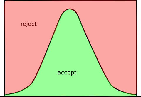
Going back to the $d$-dimensional case, let us call $\mathcal{C}_{f}$ the set of points that are under the curve of $f$. Namely, $\mathcal{C}_{f}=\{(x,y)\in\mathbb{R}^{d}\times\mathbb{R}\textnormal{ s.t. }0\leq y\leq f(x)\}$. The $\mathcal{C}_{f}$ set is the $d$-dimensional equivalent of the area under the curve. Given a pdf $f$, assume we can sample uniformly in $\mathcal{C}_{f}$. From those samples, could we obtain new samples in $\mathbb{R}^{d}$ distributed according to $f$? Looking back at the 1D example in Figure 1, it would be tempting to select the abscissa of the accepted samples. Indeed, although the accepted points are uniformly distributed in $\mathcal{C}_{f}$, the abscissa of those points are more likely to fall in regions where the value of the density is high (since there is more vertical space to sample from). Theorem 2.2 establishes that this process is indeed probabilistically correct.

Rejection sampling thus solves the problem of sampling directly from $f$ by sampling uniformly from the space under its curve. Finally, if a set $\mathcal{C}$ is known from which we can sample uniformly, then applying Theorem 2.2 and 2.2 produces samples distributed according to $f$.

Finally, we need a way to sample uniformly from the $\mathcal{C}_{f}$ set, given that we know how to sample from $f$. The 1D example in Figure 1 can once again help us visualize the process. Sampling from $f$ is sampling an abscissa. Hence, what is left to sample is the corresponding ordinate. A natural idea would be to sample uniformly above the given abscissa $z$, i.e. to get $u$ uniformly sampled on $[0,1]$ and choose $u.f(z)$ as the ordinate. Theorem 2.2 tells us that this is a correct procedure.

2.3 Application to importance mixing

Figure 2: Importance mixing using the previous generation

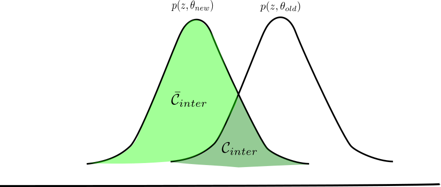
We now consider two generations $g_{old}$ and $g_{new}$ of any ES described in Section 2.1. Generation $g_{old}$ has been generated by the pdf $p(.,\mathbf{\bm{\theta}}_{old})$ and is of size $N$. We want to generate Generation $g_{new}$ according to the pdf $p(.,\mathbf{\bm{\theta}}_{new})$ and we also want it to be of size $N$. Moreover, we would like to reuse samples from generation $g_{old}$ into $g_{new}$ without biasing the samples of $g_{new}$ with respect to its pdf.

Taking a look at Figure 2, we can get the intuition of the importance mixing mechanism as follows: to sample from the pdf $p(.,\mathbf{\bm{\theta}}_{new})$, it is enough to uniformly sample from the area below its graph. This area can be split in two parts: the one that intersects with the area below the curve of the old pdf $p(.,\mathbf{\bm{\theta}}_{old})$, $\mathcal{C}_{inter}$, and its complement, $\bar{\mathcal{C}}_{inter}$. Since we already have access to samples from the pdf $p(.,\mathbf{\bm{\theta}}_{old})$, we can sample uniformly below the curve of $p(.,\mathbf{\bm{\theta}}_{old})$ and then uniformly sample from $\mathcal{C}_{inter}$.

We now need to further detail two sampling rules: one to sample uniformly from the common area $\mathcal{C}_{inter}$, and one to sample uniformly from the leftover area $\bar{\mathcal{C}}_{inter}$. Once this is done, we explain how to combine them.

2.3.1 Getting samples from the previous generation

As we stated above, to sample from the common area, we reuse samples coming from generation $g_{old}$. According to Theorem 2.2, to sample uniformly from the area below the curve of the pdf $p(.,\mathbf{\bm{\theta}}_{old})$, we only need to consider an abscissa $z$, sampled according to $p(.,\mathbf{\bm{\theta}}_{old})$, and an ordinate, obtained as $u.p(z,\mathbf{\bm{\theta}}_{old})$ where $u$ is uniformly sampled between 0 and 1. The intersection area can be formally described as

$$\mathcal{C}_{inter}=\{(z,y)\in\mathbb{R}^{d}\times\mathbb{R}\text{ s.t. }0\leq y\leq\min(p(z,\mathbf{\bm{\theta}}_{old}),p(z,\mathbf{\bm{\theta}}_{new}))\}.$$ (1)

Since $\mathcal{C}_{inter}\subset\mathcal{C}_{p(.,\mathbf{\bm{\theta}}_{old})}$, according to Theorem 2.2, to sample uniformly on $\mathcal{C}_{inter}$ one only needs to take the samples generated uniformly from $\mathcal{C}_{p(.,\mathbf{\bm{\theta}}_{old})}$ that landed in the intersection. In practice, this means that, assuming $p(z,\mathbf{\bm{\theta}}_{old})>0$, we accept $z$ in the new generation if

$$u.p(z,\mathbf{\bm{\theta}}_{old}) <min(p(z,\mathbf{\bm{\theta}}_{old}),p(z,\mathbf{\bm{\theta}}_{new})),$$ (2)

$$\text{i.e.\ }u <min(1,\frac{p(z,\mathbf{\bm{\theta}}_{new})}{p(z,\mathbf{\bm{\theta}}_{old})}).$$ (3)

This makes the first acceptance rule:

2.3.2 Sampling from the new generation

To sample uniformly from the leftover area, we follow a similar process. Since $\bar{\mathcal{C}}_{inter}\subset\mathcal{C}_{p(.,\mathbf{\bm{\theta}}_{new})}$ and $\bar{\mathcal{C}}_{inter}\cap\mathcal{C}_{p(.,\mathbf{\bm{\theta}}_{old})}=\emptyset$, we cannot reuse any more samples. Thus we must sample directly from $p(.,\mathbf{\bm{\theta}}_{new})$. We can describe the leftover region formally as

$$\bar{\mathcal{C}}_{inter}=\{(z,y)\in\mathbb{R}^{d}\times\mathbb{R}\text{ s.t. }\min(p(z,\mathbf{\bm{\theta}}_{old}),p(z,\mathbf{\bm{\theta}}_{new}))\leq y\leq p(z,\mathbf{\bm{\theta}}_{new}))\}.$$ (4)

After sampling $z$ from $p(.,\mathbf{\bm{\theta}}_{new})$, given $u$ uniformly sampled between 0 and 1 and assuming $p(z,\mathbf{\bm{\theta}}_{new})>0$, we accept $z$ in the new generation if

$$u.p(z,\mathbf{\bm{\theta}}_{new}) \geq\min(p(z,\mathbf{\bm{\theta}}_{old}),p(z,\mathbf{\bm{\theta}}_{new})),$$ (5)

$$\text{i.e.\ \quad}1-u \leq\max(0,1-\frac{p(z,\mathbf{\bm{\theta}}_{old})}{p(z,\mathbf{\bm{\theta}}_{new})}).$$ (6)

This results in the second acceptance rule:

2.3.3 Combining both sources of samples

Now assume that the $d$-dimensional volume of the intersection is equal to $\lambda$. Since $p(.,\mathbf{\bm{\theta}}_{new})$ is a pdf, the volume of the leftover area must be $1-\lambda$. If we want to sample uniformly from $\mathcal{C}_{p(.,\mathbf{\bm{\theta}}_{new})}=\mathcal{C}_{inter}\cup\bar{\mathcal{C}}_{inter}$, we need to sample uniformly from $\mathcal{C}_{inter}$ and $\bar{\mathcal{C}}_{inter}$ according to the ratio of their volume. Fortunately, when sampling uniformly from the volume below the curve of $p(.,\mathbf{\bm{\theta}}_{old})$, samples land in the intersection with probability $\lambda$. Likewise, when sampling uniformly from the volume below the curve of $p(.,\mathbf{\bm{\theta}}_{new})$, samples land in the leftover volume with probability $1-\lambda$. This means that to sample uniformly on $\mathcal{C}_{p(.,\mathbf{\bm{\theta}}_{new})}$, it is enough to simply use alternatively Rule 2.3.1 and Rule 2.3.2. The complete algorithm is described in Algorithm 2.

Algorithm 2 Importance mixing

0:  $p(z,\mathbf{\bm{\theta}}_{new})$: new pdf, $p(z,\mathbf{\bm{\theta}}_{old})$: old pdf, $g_{old}$: old generation

1:  $g_{new}\leftarrow\emptyset$

2:  for $i\leftarrow 1$ to $N$ 

2:     

3:     Draw rand1 and rand2 uniformly from $[0,1]$

4:     $z_{i}=g_{old}(i)$                                        $\triangleright$ taken uniformly from $g_{old}$

5:     if $min(1,\frac{p(z_{i},\mathbf{\bm{\theta}}_{new})}{p(z_{i},\mathbf{\bm{\theta}}_{old})})>$ rand1: 

6:        $g_{new}\leftarrow g_{new}.append(z_{i})$                            $\triangleright$ Rule 2.3.1

6:     

7:     draw $z^{\prime}_{i}\sim p(.,\mathbf{\bm{\theta}}_{new})$

8:     if $max(0,1-\frac{p(z^{\prime}_{i},\mathbf{\bm{\theta}}_{old})}{p(z^{\prime}_{i},\mathbf{\bm{\theta}}_{new})})>$ rand2: 

9:        $g_{new}\leftarrow g_{new}.append(z^{\prime}_{i})$                            $\triangleright$ Rule 2.3.2

9:     

10:     size = $|g_{new}|$

11:     if size $\geq N$:  go to 12

11:     

12:  if size $>N$:  remove a randomly chosen sample

13:  if size $<N$:  fill the generation sampling from $p(.,\mathbf{\bm{\theta}}_{new})$

14:  return  $g_{new}$

At each step of the algorithm, one alternatively tries an existing sample from $g_{old}$ and a sample drawn from $p(z,\mathbf{\bm{\theta}}_{new})$. Both samples can be either accepted or rejected according to Rules 2.3.1 and 2.3.2 respectively.

Given that we are sampling from two sources at each step, it may happen that, when Generation $g_{new}$ already contains $N-1$ samples, two samples are accepted at the last iteration and we get a generation with $N+1$ samples. In that case, it is necessary to remove one sample, which can be randomly chosen.

If one applies the above process $N$ times then, on average, $(1-\lambda)N$ samples will be accepted from $g_{old}$ and $\lambda N$ samples will be accepted from $p(z,\mathbf{\bm{\theta}}_{new})$, thus on average the size of the obtained generation $g_{new}$ will be $N$. In practice however, samples may be accepted faster or more slowly than on average. If they are accepted faster, this means that Generation $g_{new}$ will contain $N$ samples before the above process has been run $N$ times. If they are accepted more slowly, this means that Generation $g_{new}$ will contain less than $N$ samples after the above process has been run $N$ times (which means that all samples from $g_{old}$ have been tried).

In that context, Sun et al. (2009) propose instead to first exhaust the old generation using Rule 2.3.1, resulting in $N_{\beta}\leq N$ samples. Then, they use Rule 2.3.2 repeatedly until they get $N-N_{\beta}$ new samples. On average, $N$ trials are needed, but it is often the case that more than $N$ or less than $N$ trials are performed, and in these common cases a bias is introduced, as the samples in $\mathcal{C}_{inter}$ and $\bar{\mathcal{C}}_{inter}$ are not well balanced.

A more satisfactory option consists in completing Generation $g_{new}$ with samples drawn directly from $p(z,\mathbf{\bm{\theta}}_{new})$ (accepting them all) until it is full. Another option consists in applying the correct importance mixing process that we have outlined above, but using other existing generations, as proposed in Section 3.

Note that Sun et al. (2009) also use a ”minimal refresh rate” parameter $\alpha$ which is set to 0 in our description here, as a different value may only deteriorate sample reuse.

2.3.4 Complexity of importance mixing

The complexity of the algorithm can be deduced as follows: in the case where the pdfs are multivariate Gaussian functions, accepting a sample $z$ with probability $\frac{p(z,\mathbf{\bm{\theta}}_{new})}{p(z,\mathbf{\bm{\theta}}_{old})}$ can be written

$$random<\sqrt{\frac{det(\Sigma_{old})}{det(\Sigma_{new})}}e^{\frac{1}{2}(\mu_{new}-z)^{T}\Sigma_{new}^{-1}(\mu_{new}-z)-\frac{1}{2}(\mu_{old}-z)^{T}\Sigma_{old}^{-1}(\mu_{old}-z)}.$$

Computing the ratio thus involves twice the evaluation of the same determinant, and twice the same matrix inversion, as well as four matrix-vector products, so the global complexity is in $O(4d^{2.373})+Nd^{2})$.

One can see that the importance mixing mechanism scales poorly with the dimension of the optimization problem. However, in the case where only diagonal covariance matrices are considered, the complexity can be scaled down to $\mathcal{O}(Nd)$, which is much more affordable in practice.

2.4 Impact on sampling efficiency

In terms of sample efficiency, the main point about using importance mixing is that only the new samples drawn from $p(.,\mathbf{\bm{\theta}}_{new})$ need to be evaluated by running the system, as the value of samples from $g_{old}$ is already known. Thus, approximately, only $\lambda N$ samples are evaluated instead of $N$ at each generation. However, depending on the ES algorithm, some of the samples from $g_{old}$ might not effectively be reused. In open-es and snes, all samples are reused to compute the approximation of the gradients. By contrast, in CEM and CMAES, only the $K_{e}$ elite individuals of the population are used in practice. One may think that this phenomenon somehow hampers sample reuse. However, whatever the fate of samples from $g_{old}$, all samples from $g_{new}$ need to be evaluated, thus ignoring samples from $g_{old}$ has no impact on sample efficiency.

3 Extending Importance Mixing to multiple generations

Figure 3: Extended Importance mixing, using several generations

As outlined above, it may happen (roughly half of the time) that after using samples from the previous generation, the new generation is still not full. In that case, samples from former generations could be used to continue filling it while using as few samples from $p(z,\mathbf{\bm{\theta}}_{new})$ as possible, as illustrated in Figure 3.

This alternative option is described in Algorithm 3.

Algorithm 3 Extended Importance mixing

0:  $p(z,\mathbf{\bm{\theta}}_{new})$: new pdf, K: number of generations considered in the archive

0:  for $k\in\{1,\dots,K\}$ $p(z,\mathbf{\bm{\theta}}^{k}_{old})$: $k^{th}$ old pdf, $g^{k}_{old}$: $k^{th}$ old generation

1:  $g_{new}\leftarrow\emptyset$

2:  for $k\leftarrow 1$ to $K$ 

3:     for $i\leftarrow 1$ to $N$ 

3:        

4:        Draw rand1 and rand2 uniformly from $[0,1]$

5:        $z_{i}=g^{k}_{old}(i)$                                        $\triangleright$ taken uniformly from $g^{k}_{old}$

6:        if $\min(1,\frac{p(z_{i},\mathbf{\bm{\theta}}_{new})}{p(z_{i},\mathbf{\bm{\theta}}^{k}_{old})})>$ rand1: 

7:           $g_{new}\leftarrow g_{new}.append(z_{i})$                            $\triangleright$ Rule 2.3.1

7:        

8:        draw $z^{\prime}_{i}$ from $p(.,\mathbf{\bm{\theta}}_{new})$

9:        if $\max(0,1-\frac{p(z^{\prime}_{i},\mathbf{\bm{\theta}}^{k}_{old})}{p(z^{\prime}_{i},\mathbf{\bm{\theta}}_{new})})>$ rand2: 

10:           $g_{new}\leftarrow g_{new}.append(z^{\prime}_{i})$                            $\triangleright$ Rule 2.3.2

10:        

11:        size = $|g_{new}|$

12:        if size $\geq N$:  go to 13

12:  

13:  if size $>N$:  remove a randomly chosen sample

14:  return  $g_{new}$

4 Experimental study

In this section we investigate the effect of the importance mixing mechanism and its extended version on sample efficiency. We use the open-es, snes, cem and cma-es evolutionary algorithms presented in Section 2.1.

4.1 Experimental setup

To evaluate sample efficiency, we use the CartPole and Acrobot environments from the OpenAI gym benchmark.

In CartPole, a pole is attached to a cart, which is allowed to move along the x-axis. The state information contains the position and velocity of the cart, the velocity of the tip of the pole, and the angle between the pole and the vertical line. At each time step, the agent chooses to push the cart to the left or to the right, with a force of respectively -1 and +1 unit. It receives of reward of +1 at each step, until the episode ends, when either the angle between the pole and the vertical line exceeds 15 degrees, the cart moves more than 2.4 units away from the center, or 200 time steps have elapsed. The maximum possible reward over an episode is thus 200.

In Acrobot, the agent must control a double pendulum (two joints and two links) allowed to move in the xy-plane. Initially, the links are hanging downwards. The state information contains the sine and cosine of the two rotational joint angles and the angular velocities of the two links. At each time step, the agent applies a torque of either -1, 0 or +1 to the joint between the two links. It receives a reward of -1 at each time step, until the episode ends, when either the tip of the second link gets higher than one link above the center joint, or 200 time steps have elapsed. The maximum possible reward in this environment is not known.

Policies $\pi_{\mathbf{\bm{\theta}}}$ are represented by a small neural network with 2 hidden layers of size 8, making for a total of respectively 130 and 155 parameters to be tuned by the evolutionary algorithms for the CartPole and Acrobot environments.

The size of the ES populations is set to 50 and, for all algorithms, the initial covariance is set to $\sigma^{2}\mathcal{I}_{d}$, where $\sigma=0.25$. For the algorithms relying on gradient descent (open-es and snes), we use Adam with an initial learning rate of 0.01, and set the hyper-parameters $\beta_{1}$ and $\beta_{2}$ (see Kingma and Ba (2014) for more details on the algorithm) to $0.99$ and $0.999$ respectively.

We also use a ranking mechanism: instead of raw fitness, we associate to the individuals their rank in the population (fitness-wise). This means that the ES algorithm aims at having individuals with good ranks (and thus good fitness), and it has the advantage to remove the influence of outliers in the population (Stulp and Sigaud, 2012a). Finally, we add weight decay for regularization in all algorithms, which translates into a negative penalty to prevent the weights of the neural networks from being too large. This penalty is computed as $-0.05||\theta||^{2}$, where $\theta$ is the corresponding set of parameters.

We let each algorithm run for a fixed number of generations: 1000 for open-es and snes, and 400 for cma-es and cem. We do this once with the EIM included, and once without it, and repeat the process for both environments. Results are averaged over 25 runs with different random seeds. The displayed variance corresponds to the $68\%$ confidence interval for the estimation of the mean.

4.2 Results

The evolution of the average performance of the population of each algorithm can be seen in Figure 4a, 4b for the CartPole environment, and Figure 5a, 5b for the Acrobot environment. One can see that in general, algorithms have no difficulties finding good policies, but on the CartPole task, cem seems to get stuck into local maxima.

(a)

(b)

Figure 4: Evolution of the average score of the population over iterations of the algorithms without (a) and with (b) the extended importance mixing mechanism on CartPole.

(a)

(b)

Figure 5: Evolution of the average score of the population over iterations of the algorithms without (a) and with (b) the extended importance mixing mechanism, on Acrobot.

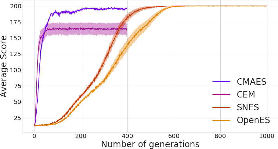
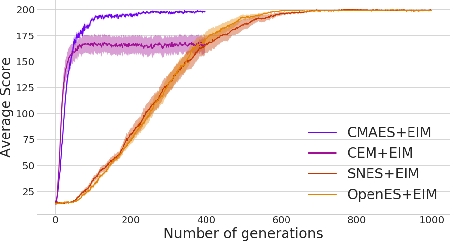
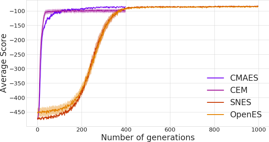
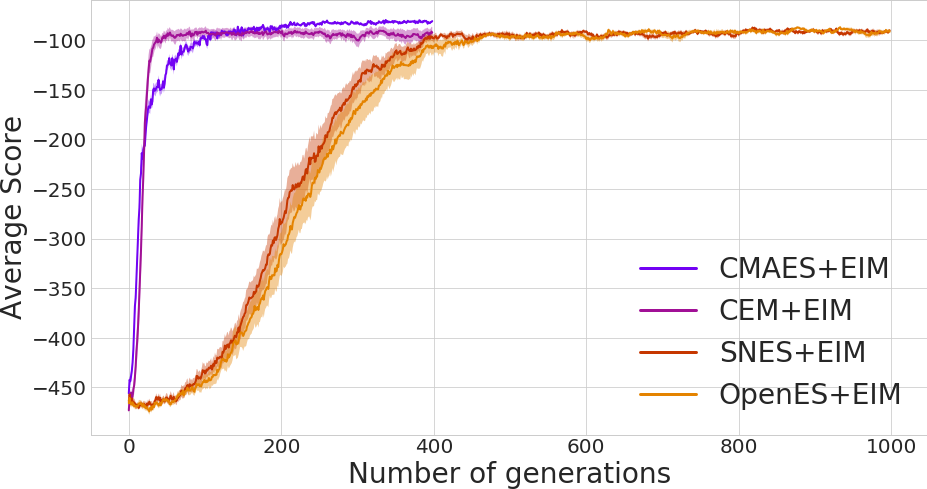
On CartPole, without the EIM mechanism, the maximum possible reward of $200$ is reached in around $500$ generations with snes and $600$ with open-es. Interestingly, cma-es only reaches an average performance around $195$ after $400$ generations whereas cem gets stuck around $160$ after $100$ generations. With the EIM mechanism, results are very similar, indicating that EIM does not hurt convergence. On the Acrobot environment, without the EIM mechanism, rewards of around $-90$ are reached in $400$ generations with snes and open-es, and $50$ generations with cem. cma-es slightly outperforms the other algorithms, reaching a fitness around $-75$ in $200$ generations. Again, the impact of the EIM mechanism on the convergence of the algorithms is limited.

However, the key quantity in this study is the number of sample evaluations required to achieve convergence. In 6a, 6b, and Figure 7a, 7b, we report the evolution of the average score of the population for all algorithms and both benchmarks, using as time scale the number of samples evaluated from the system, rather than the number of sampled populations.

(a)

(b)

Figure 6: Evolution of the average score of the population over the number of evaluated episodes without (a) and with (b) the extended importance mixing mechanism on CartPole.

(a)

(b)

Figure 7: Evolution of the average score of the population over the number of evaluated episodes without (a) and with (b) the extended importance mixing mechanism on Acrobot.

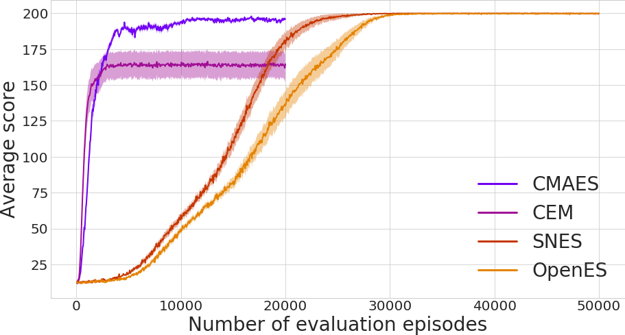
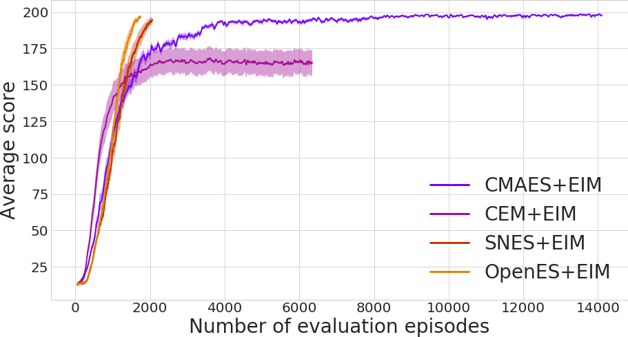
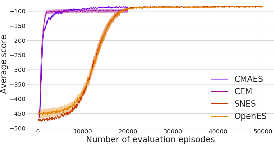
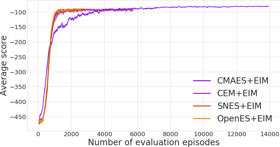
One can see that the EIM mechanism allows for a substantial speedup in convergence. On CartPole, the total number of evaluations goes down from 20000 to 14000 for cma-es, 20000 to 6000 for cem and from 50000 to $2000$ for snes and open-es. However, as detailed below, this speedup mostly comes from the IM rather than from its extension.

In Table 1, we report the percentage of evaluations that were reused from the previous generation using the importance mixing mechanism and the percentage of evaluations that were reused from the generation preceding the previous generation using the extended importance mixing mechanism. To compute those statistics, we monitored over runs the number of samples reused per generation, and the number of reused samples that came from the EIM.

	CartPole Environment			Acrobot Environment
	Total reuse	from IM	from EIM	Total reuse	from IM	from EIM
cma-es	$29.2\%$	$100\%$	$0.0\%$	$29.4\%$	$100\%$	$0.0\%$
cem	$50.6\%$	$90.0\%$	$10.0\%$	$48.0\%$	$89.6\%$	$10.4\%$
snes	$95.2\%$	$96.6\%$	$3.4\%$	$93.4\%$	$96.8\%$	$3.2\%$
open-es	$95.9\%$	$97.2\%$	$2.8\%$	$94.4\%$	$97.2\%$	$2.8\%$

Table 1: Sample reuse using importance mixing (IM) and extended importance mixing (EIM) on the CartPole and Acrobot environments. Reuse percentages from IM and from EIM are subparts of the total reuse.

From Table 1, one can see that in both tasks, open-es and snes reach excellent reuse rates over $95\%$, meaning that less than one out of ten samples has to be evaluated. On both benchmarks, cma-es and cem lag behind with around $30\%$ and $50\%$ sample reuse, which is still non-negligible. Notice that in any case, only around $5\%$ of the reused samples come from the EIM. This quantity is at its maximum and reaches $10.0\%$ and $10.4\%$ for the cem algorithm, and at its lowest with cma-es where it is stuck at $0\%$. The boost in sample reuse is thus almost imperceptible.

In this setting, the high reuse rates make open-es and snes particularly efficient in terms of the number of evaluations, giving them convergence speeds on par with cma-es and cem. Their linear complexity also makes them much more affordable in high-dimension.

The fact that the extended importance mixing mechanism does not bring significant improvement over standard importance mixing can be explained easily. On average, standard importance mixing completely fills the new generation half of the time. When the new generation is not full yet, generally very few samples are missing. Then the probability that it is still not full after filling from the second generation is very low and using a third generation is almost never necessary.

4.3 Comparison to deep reinforcement learning

Deep reinforcement learning (deep RL) approaches are considered more sample efficient than evolutionary approaches (Sigaud and Stulp, 2018). Being step-based, as opposed to episode-based evolutionary algorithms, deep RL methods make a better use of their sample information. In this study, we use ddpg, an off-policy and sample efficient deep RL algorithm which uses a replay buffer to reuse samples and improve stability (Lillicrap et al., 2015). Thus we train a ddpg agent and compare its sample efficiency with an evolutionary algorithm using the importance mixing mechanism. ddpg is designed to solve continuous action RL problems, so for this experiment we work on a continuous version of the CartPole environment. The original CartPole only accepts forces of -1 and +1. Here we relax this constraint by allowing a continuous-valued force in $[-1,1]$.

We choose to use the snes + EIM algorithm for this study, as Figures 6 and 7 show that it converged with a competitive number of samples with respect to cma-es + EIM. Besides, using a diagonal covariance matrix makes the training faster, whilst allowing for more expressiveness than the simple open-es algorithm. To limit the computational cost, we performed a limited grid-search over the population size, the initial covariance, and the learning rate of the Adam optimizer.

Figure 8: Average score of the population using snes + EIM as the number of sample evaluations increases for different population sizes. The learning rate is $0.01$ and the initial covariance is $0.1^{2}\mathcal{I}_{d}$.

Figure 9: Average score of the population using snes + EIM as the number of sample evaluations increases for different values of $\sigma$. The learning rate is $0.01$ and the population size is 25.

Figure 10: Average score of the population using snes + EIM as the number of sample evaluations increases for different values of learning rate (lr). The population size is 25 and the initial covariance is $0.1^{2}\mathcal{I}_{d}$.

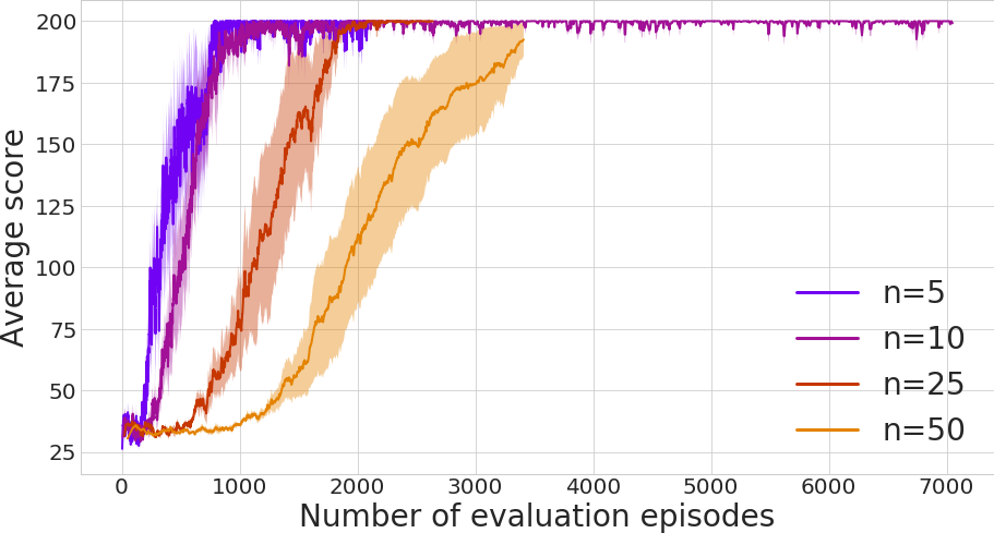
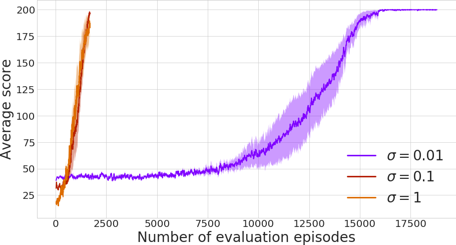
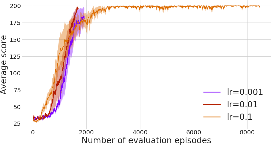
The influence of the population size can be seen in Figure 8, the influence of $\sigma$ in Figure 9, and the influence of the learning rate in Figure 10. Selecting $popsize=10,\sigma=0.1$ and $lr=0.1$ gives the best results (in terms of convergence speed and stability), with the algorithm converging after around 1500 evaluations.

Then we trained a ddpg agent on the Continuous CartPole environment, using standard ddpg parameters as provided in the baselines (Dhariwal et al., 2017). Besides, to allow for a fair comparison, the actor had the same architecture as the evolved policy (two hidden layers of size 8). However, we found that we had to increase the size of the hidden layers of the critic to 16 in order for the algorithm to converge. The learning rate of the actor and the critic were respectively set to $0.005$ and $0.01$. The soft-target update parameter was set to $\tau=0.001$, and the discount rate to $\gamma=0.99$. Exploration was ensured with an Ornstein-Uhlenbeck process (Uhlenbeck and Ornstein, 1930), as proposed in the original ddpg paper (Lillicrap et al., 2015).

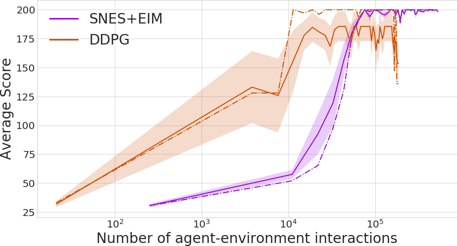
The snes + EIM algorithm was run for 1500 generations whereas ddpg was run for 1000 episodes, which is enough in both cases to reach convergence. The evolution of the performance of snes + EIM and ddpg over the number of steps sampled from the system can be seen in Figure 11a. One can see that ddpg converges around 10 times faster than snes + EIM on this benchmark. Even with a sample reuse rate of around $90\%$, the gap between evolutionary algorithms and deep RL is still important. However, ddpg is somehow more unstable than snes + EIM. It sometimes happens that the algorithm diverges late in the experiment, in contrast to the evolutionary method.

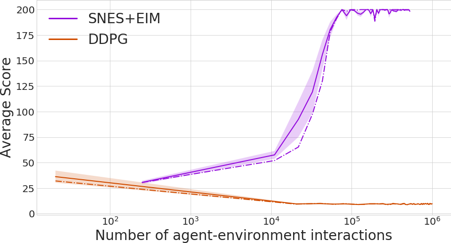
However, the Continuous Cartpole benchmark is favorable to deep RL methods, since the reward signal is very dense (one reward per step). By contrast, evolutionary algorithms really shine when rewards are sparse, since they only take into account rewards over episodes when enhancing their policies. We thus finally compared ddpg and snes + EIM on another environment that we call ”ContinuousCartPoleHard”. In this environment, the agent only receives the total reward after the episode ends. We used the same hyper-parameters for both algorithms, and let snes + EIM run for 1500 generations, and ddpg for 1 million time steps. The change had no influence over the evolutionary algorithms, while it turned out to be much more challenging for the ddpg agent, as can be seen in Figure 11b where ddpg does not make any progress.

(a)

(b)

Figure 11: Average score of the population as the number of sample evaluations increases on the ContinuousCartPole (a) and ContinuousCartPoleHard (b) environments. Dotted lines correspond to medians. For better visualization, we use a log scale over the x-axis.

5 Conclusion and future work

In this paper we have given a didactic presentation of an improved version of the importance mixing mechanism initially published in Sun et al. (2009), and we have explained how it could be extended to make profit of the samples coming from several generations.

The experimental study revealed that, on one side, the basic importance mixing mechanism provides significant sample efficiency improvement but, on the other side, the extended importance mixing mechanism does not bring this improvement much further. Besides, importance mixing alone is not enough for evolutionary strategies to compete with deep RL methods in terms of sample efficiency. However, as already noted several times in the literature, evolutionary methods are generally more stable than deep RL methods.

Based on these conclusions, in future work we intend to turn towards frameworks where evolutionary methods and deep RL methods are combined, such as Khadka and Tumer (2018) and Colas et al. (2018). In both cases, the evolutionary part is not based on an evolutionary strategy, thus the importance mixing mechanism cannot be applied straightforwardly to these combinations. This will be the focus of our next research effort.

References

- Akimoto et al. (2010) Akimoto, Y., Nagata, Y., Ono, I., Kobayashi, S., 2010. Bidirectional relation between cma evolution strategies and natural evolution strategies. In: International Conference on Parallel Problem Solving from Nature. Springer, pp. 154–163.
- Arnold et al. (2011) Arnold, L., Auger, A., Hansen, N., Ollivier, Y., 2011. Information-geometric optimization algorithms: A unifying picture via invariance principles. Tech. rep., INRIA Saclay.
- Back (1996) Back, T., 1996. Evolutionary algorithms in theory and practice: evolution strategies, evolutionary programming, genetic algorithms. Oxford university press.
- Colas et al. (2018) Colas, C., Sigaud, O., Oudeyer, P.-Y., 2018. GEP-PG: Decoupling exploration and exploitation in deep reinforcement learning algorithms. arXiv preprint arXiv:1802.05054.
- Conti et al. (2017) Conti, E., Madhavan, V., Such, F. P., Lehman, J., Stanley, K. O., Clune, J., 2017. Improving exploration in evolution strategies for deep reinforcement learning via a population of novelty-seeking agents. arXiv preprint arXiv:1712.06560.
- Deisenroth et al. (2013) Deisenroth, M. P., Neumann, G., Peters, J., et al., 2013. A survey on policy search for robotics. Foundations and Trends® in Robotics 2 (1–2), 1–142.
- Dhariwal et al. (2017) Dhariwal, P., Hesse, C., Klimov, O., Nichol, A., Plappert, M., Radford, A., Schulman, J., Sidor, S., Wu, Y., 2017. OpenAI baselines. \urlhttps://github.com/openai/baselines.
- Glasmachers et al. (2010) Glasmachers, T., Schaul, T., Yi, S., Wierstra, D., Schmidhuber, J., 2010. Exponential natural evolution strategies. In: Proceedings of the 12th annual conference on Genetic and evolutionary computation. ACM, pp. 393–400.
- Khadka and Tumer (2018) Khadka, S., Tumer, K., 2018. Evolutionary reinforcement learning. arXiv preprint arXiv:1805.07917.
- Kingma and Ba (2014) Kingma, D. P., Ba, J., 2014. Adam: A method for stochastic optimization. arXiv preprint arXiv:1412.6980.
- Larrañaga and Lozano (2001) Larrañaga, P., Lozano, J. A., 2001. Estimation of distribution algorithms: A new tool for evolutionary computation. Vol. 2. Springer Science & Business Media.
- Lillicrap et al. (2015) Lillicrap, T. P., Hunt, J. J., Pritzel, A., Heess, N., Erez, T., Tassa, Y., Silver, D., Wierstra, D., 2015. Continuous control with deep reinforcement learning. arXiv preprint arXiv:1509.02971.
- Petroski Such et al. (2017) Petroski Such, F., Madhavan, V., Conti, E., Lehman, J., Stanley, K. O., Clune, J., 2017. Deep neuroevolution: Genetic algorithms are a competitive alternative for training deep neural networks for reinforcement learning. arXiv preprint arXiv:1712.06567.
- Salimans et al. (2017) Salimans, T., Ho, J., Chen, X., Sutskever, I., 2017. Evolution strategies as a scalable alternative to reinforcement learning. arXiv preprint arXiv:1703.03864.
- Salimans and Kingma (2016) Salimans, T., Kingma, D. P., 2016. Weight normalization: A simple reparameterization to accelerate training of deep neural networks. arXiv preprint arXiv:1602.07868.
- Schaul et al. (2011) Schaul, T., Glasmachers, T., Schmidhuber, J., 2011. High dimensions and heavy tails for natural evolution strategies. In: GECCO.
- Schulman et al. (2015) Schulman, J., Levine, S., Moritz, P., Jordan, M. I., Abbeel, P., 2015. Trust region policy optimization. CoRR, abs/1502.05477.
- Schulman et al. (2017) Schulman, J., Wolski, F., Dhariwal, P., Radford, A., Klimov, O., 2017. Proximal policy optimization algorithms. arXiv preprint arXiv:1707.06347.
- Sigaud and Stulp (2018) Sigaud, O., Stulp, F., 2018. Policy search in continuous action domains: an overview. arXiv preprint arXiv:1803.04706.
- Stulp and Sigaud (2012a) Stulp, F., Sigaud, O., 2012a. Path integral policy improvement with covariance matrix adaptation. In: Proceedings of the 29th International Conference on Machine Learning. Edinburgh, Scotland, pp. 1–8.
- Stulp and Sigaud (2012b) Stulp, F., Sigaud, O., 2012b. Policy improvement methods: Between black-box optimization and episodic reinforcement learning. Tech. rep., hal-00738463.
- Stulp and Sigaud (2013) Stulp, F., Sigaud, O., august 2013. Robot skill learning: From reinforcement learning to evolution strategies. Paladyn Journal of Behavioral Robotics 4 (1), 49–61.
- Sun et al. (2009) Sun, Y., Wierstra, D., Schaul, T., Schmidhuber, J., 2009. Efficient natural evolution strategies. In: Proceedings of the 11th Annual conference on Genetic and evolutionary computation. ACM, pp. 539–546.
-
Uhlenbeck and Ornstein (1930)
Uhlenbeck, G. E., Ornstein, L. S., Sep 1930. On the theory of the brownian
motion. Phys. Rev. 36, 823–841.
URL \urlhttps://link.aps.org/doi/10.1103/PhysRev.36.823 - Wierstra et al. (2008) Wierstra, D., Schaul, T., Peters, J., Schmidhuber, J., 2008. Natural evolution strategies. In: IEEE Congress on Evolutionary Computation. IEEE, pp. 3381–3387.