Population Based Training of Neural Networks
Abstract
Neural networks dominate the modern machine learning landscape, but their training and success still suffer from sensitivity to empirical choices of hyperparameters such as model architecture, loss function, and optimisation algorithm. In this work we present Population Based Training (PBT), a simple asynchronous optimisation algorithm which effectively utilises a fixed computational budget to jointly optimise a population of models and their hyperparameters to maximise performance. Importantly, PBT discovers a schedule of hyperparameter settings rather than following the generally sub-optimal strategy of trying to find a single fixed set to use for the whole course of training. With just a small modification to a typical distributed hyperparameter training framework, our method allows robust and reliable training of models. We demonstrate the effectiveness of PBT on deep reinforcement learning problems, showing faster wall-clock convergence and higher final performance of agents by optimising over a suite of hyperparameters. In addition, we show the same method can be applied to supervised learning for machine translation, where PBT is used to maximise the BLEU score directly, and also to training of Generative Adversarial Networks to maximise the Inception score of generated images. In all cases PBT results in the automatic discovery of hyperparameter schedules and model selection which results in stable training and better final performance.
DeepMind, London, UK
1 Introduction
Neural networks have become the workhorse non-linear function approximator in a number of machine learning domains, most notably leading to significant advances in reinforcement learning (RL) and supervised learning. However, it is often overlooked that the success of a particular neural network model depends upon the joint tuning of the model structure, the data presented, and the details of how the model is optimised. Each of these components of a learning framework is controlled by a number of parameters, hyperparameters, which influence the learning process and must be properly tuned to fully unlock the network performance. This essential tuning process is computationally expensive, and as neural network systems become more complicated and endowed with even more hyperparameters, the burden of this search process becomes increasingly heavy. Furthermore, there is yet another level of complexity in scenarios such as deep reinforcement learning, where the learning problem itself can be highly non-stationary (e.g. dependent on which parts of an environment an agent is currently able to explore). As a consequence, it might be the case that the ideal hyperparameters for such learning problems are themselves highly non-stationary, and should vary in a way that precludes setting their schedule in advance.
Two common tracks for the tuning of hyperparameters exist: parallel search and sequential optimisation, which trade-off concurrently used computational resources with the time required to achieve optimal results. Parallel search performs many parallel optimisation processes (by optimisation process we refer to neural network training runs), each with different hyperparameters, with a view to finding a single best output from one of the optimisation processes – examples of this are grid search and random search. Sequential optimisation performs few optimisation processes in parallel, but does so many times sequentially, to gradually perform hyperparameter optimisation using information obtained from earlier training runs to inform later ones – examples of this are hand tuning and Bayesian optimisation. Sequential optimisation will in general provide the best solutions, but requires multiple sequential training runs, which is often unfeasible for lengthy optimisation processes.
In this work, we present a simple method, Population Based Training (PBT) which bridges and extends parallel search methods and sequential optimisation methods. Advantageously, our proposal has a wall-clock run time that is no greater than that of a single optimisation process, does not require sequential runs, and is also able to use fewer computational resources than naive search methods such as random or grid search. Our approach leverages information sharing across a population of concurrently running optimisation processes, and allows for online propagation/transfer of parameters and hyperparameters between members of the population based on their performance. Furthermore, unlike most other adaptation schemes, our method is capable of performing online adaptation of hyperparameters – which can be particularly important in problems with highly non-stationary learning dynamics, such as reinforcement learning settings. PBT is decentralised and asynchronous, requiring minimal overhead and infrastructure. While inherently greedy, we show that this meta-optimisation process results in effective and automatic tuning of hyperparameters, allowing them to be adaptive throughout training. In addition, the model selection and propagation process ensures that intermediate good models are given more computational resources, and are used as a basis of further optimisation and hyperparameter search.
We apply PBT to a diverse set of problems and domains to demonstrate its effectiveness and wide applicability. Firstly, we look at the problem of deep reinforcement learning, showing how PBT can be used to optimise UNREAL (Jaderberg et al., 2016) on DeepMind Lab levels (Beattie et al., 2016), Feudal Networks (Vezhnevets et al., 2017) on Atari games (Bellemare et al., 2013), and simple A3C agents for StarCraft II (Vinyals et al., 2017). In all three cases we show faster learning and higher performance across a suite of tasks, with PBT allowing discovery of new state-of-the-art performance and behaviour, as well as the potential to reduce the computational resources for training. Secondly, we look at its use in supervised learning for machine translation on WMT 2014 English-to-German with Transformer networks (Vaswani et al., 2017), showing that PBT can match and even outperform heavily tuned hyperparameter schedules by optimising for BLEU score directly. Finally, we apply PBT to the training of Generative Adversarial Networks (GANs) (Goodfellow et al., 2014) by optimising for the Inception score (Salimans et al., 2016) – the result is stable GAN training with large performance improvements over a strong, well-tuned baseline with the same architecture (Radford et al., 2016).
The improvements we show empirically are the result of (a) automatic selection of hyperparameters during training, (b) online model selection to maximise the use of computation spent on promising models, and (c) the ability for online adaptation of hyperparameters to enable non-stationary training regimes and the discovery of complex hyperparameter schedules.
In Sect. 2 we review related work on parallel and sequential hyperparameter optimisation techniques, as well as evolutionary optimisation methods which bear a resemblance to PBT. We introduce PBT in Sect. 3, outlining the algorithm in a general manner which is used as a basis for experiments. The specific incarnations of PBT and the results of experiments in different domains are given in Sect. 4, and finally we conclude in Sect. 5.
2 Related Work
First, we review the methods for sequential optimisation and parallel search for hyperparameter optimisation that go beyond grid search, random search, and hand tuning. Next, we note that PBT inherits many ideas from genetic algorithms, and so highlight the literature in this space.
The majority of automatic hyperparameter tuning mechanisms are sequential optimisation methods: the result of each training run with a particular set of hyperparameters is used as knowledge to inform the subsequent hyperparameters searched. A lot of previous work uses a Bayesian optimisation framework to incorporate this information by updating the posterior of a Bayesian model of successful hyperparameters for training – examples include GP-UCB (Srinivas et al., 2009), TPE (Bergstra et al., 2011), Spearmint (Snoek et al., 2012), and SMAC (Hutter et al., 2011). As noted in the previous section, their sequential nature makes these methods prohibitively slow for expensive optimisation processes. For this reason, a number of methods look to speed up the updating of the posterior with information from each optimisation process by performing early stopping, using intermediate losses to predict final performance, and even modelling the entire time and data dependent optimisation process in order to reduce the number of optimisation steps required for each optimisation process and to better explore the space of promising hyperparameters (György & Kocsis, 2011; Agarwal et al., 2011; Sabharwal et al., 2016; Swersky et al., 2013, 2014; Domhan et al., 2015; Klein et al., 2016; Snoek et al., 2015; Springenberg et al., 2016).
Many of these Bayesian optimisation approaches can be further sped up by attempting to parallelise them – training independent models in parallel to quicker update the Bayesian model (though potentially introducing bias) (Shah & Ghahramani, 2015; González et al., 2016; Wu & Frazier, 2016; Rasley et al., 2017; Golovin et al., 2017) – but these will still require multiple sequential model optimisations. The same problem is also encountered where genetic algorithms are used in place of Bayesian optimisation for hyperparameter evolution (Young et al., 2015).
Moving away from Bayesian optimisation, even approaches such as Hyperband (Li et al., 2016) which model the problem of hyperparameter selection as a many-armed bandit, and natively incorporate parallelisation, cannot practically be executed within a single training optimisation process due to the large amount of computational resources they would initially require.
The method we present in this paper only requires a single training optimisation process – it builds upon the unreasonable success of random hyperparameter search which has shown to be very effective (Bergstra & Bengio, 2012). Random search is effective at finding good regions for sensitive hyperparameters – PBT identifies these and ensures that these areas are explored more using partially trained models (e.g. by copying their weights). By bootstrapping the evaluation of new hyperparameters during training on partially trained models we eliminate the need for sequential optimisation processes that plagues the methods previously discussed. PBT also allows for adaptive hyperparameters during training, which has been shown, especially for learning rates, to improve optimisation (Loshchilov & Hutter, 2016; Smith, 2017; Massé & Ollivier, 2015).
PBT is perhaps most analogous to evolutionary strategies that employ self-adaptive hyperparameter tuning to modify how the genetic algorithm itself operates (Bäck, 1998; Spears, 1995; Gloger, 2004; Clune et al., 2008) – in these works, the evolutionary hyperparameters were mutated at a slower rate than the parameters themselves, similar to how hyperparameters in PBT are adjusted at a slower rate than the parameters. In our case however, rather than evolving the parameters of the model, we train them partially with standard optimisation techniques (e.g. gradient descent). Other similar works to ours are Lamarckian evolutionary algorithms in which parameters are inherited whilst hyperparameters are evolved (Castillo et al., 2006) or where the hyperparameters, initial weights, and architecture of networks are evolved, but the parameters are learned (Castillo et al., 1999; Husken et al., 2000), or where evolution and learning are both applied to the parameters (Ku & Mak, 1997; Houck et al., 1997; Igel et al., 2005). This mixture of learning and evolutionary-like algorithms has also been explored successfully in other domains (Zhang et al., 2011) such as neural architecture search (Real et al., 2017; Liu et al., 2017), feature selection (Xue et al., 2016), and parameter learning (Fernando et al., 2016). Finally, there are parallels to work such as salustowicz1997probabilistic which perform program search with genetic algorithms.
3 Population Based Training
The most common formulation in machine learning is to optimise the parameters of a model to maximise a given objective function , (e.g. classification, reconstruction, or prediction). Generally, the trainable parameters are updated using an optimisation procedure such as stochastic gradient descent. More importantly, the actual performance metric that we truly care to optimise is often different to , for example could be accuracy on a validation set, or BLEU score as used in machine translation. The main purpose of PBT is to provide a way to optimise both the parameters and the hyperparameters jointly on the actual metric that we care about.
To that end, firstly we define a function eval that evaluates the objective function, , using the current state of model . For simplicity we ignore all terms except , and define eval as function of trainable parameters only. The process of finding the optimal set of parameters that maximise is then:
| (1) |
Note that in the methods we are proposing, the eval function does not need to be differentiable, nor does it need to be the same as the function used to compute the iterative updates in the optimisation steps which we outline below (although they ought to be correlated).
When our model is a neural network, we generally optimise the weights in an iterative manner, e.g. by using stochastic gradient descent on the objective function . Each step of this iterative optimisation procedure, step, updates the parameters of the model, and is itself conditioned on some parameters (often referred to as hyperparameters).
In more detail, iterations of parameter update steps:
| (2) |
are chained to form a sequence of updates that ideally converges to the optimal solution
| (3) |
This iterative optimisation process can be computationally expensive, due to the number of steps required to find as well as the computational cost of each individual step, often resulting in the optimisation of taking days, weeks, or even months. In addition, the solution is typically very sensitive to the choice of the sequence of hyperparemeters . Incorrectly chosen hyperparameters can lead to bad solutions or even a failure of the optimisation of to converge. Correctly selecting hyperparameters requires strong prior knowledge on to exist or to be found (most often through multiple optimisation processes with different ). Furthermore, due to the dependence of on iteration step, the number of possible values grows exponentially with time. Consequently, it is common practise to either make all equal to each other (e.g. constant learning rate through entire training, or constant regularisation strength) or to predefine a simple schedule (e.g. learning rate annealing). In both cases one needs to search over multiple possible values of
| (4) |
As a way to perform (4) in a fast and computationally efficient manner, we consider training models forming a population which are optimised with different hyperparameters . The objective is to therefore find the optimal model across the entire population. However, rather than taking the approach of parallel search, we propose to use the collection of partial solutions in the population to additionally perform meta-optimisation, where the hyperparameters and weights are additionally adapted according to the performance of the entire population.
In order to achieve this, PBT uses two methods called independently on each member of the population (each worker): exploit, which, given performance of the whole population, can decide whether the worker should abandon the current solution and instead focus on a more promising one; and explore, which given the current solution and hyperparameters proposes new ones to better explore the solution space.
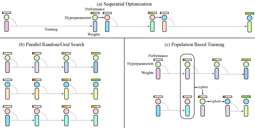
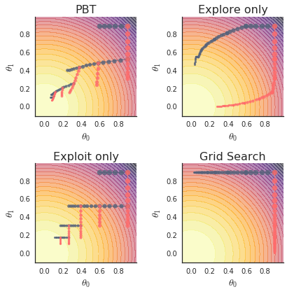
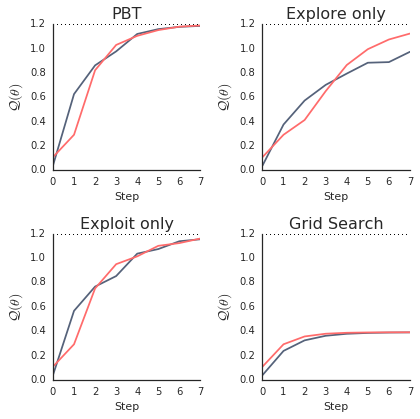
Each member of the population is trained in parallel, with iterative calls to step to update the member’s weights and eval to measure the member’s current performance. However, when a member of the population is deemed ready (for example, by having been optimised for a minimum number of steps or having reached a certain performance threshold), its weights and hyperparameters are updated by exploit and explore. For example, exploit could replace the current weights with the weights that have the highest recorded performance in the rest of the population, and explore could randomly perturb the hyperparameters with noise. After exploit and explore, iterative training continues using step as before. This cycle of local iterative training (with step) and exploitation and exploration using the rest of the population (with exploit and explore) is repeated until convergence of the model. Algorithm 1 describes this approach in more detail, Fig. 1 schematically illustrates this process (and contrasts it with sequential optimisation and parallel search), and Fig. 2 shows a toy example illustrating the efficacy of PBT.
The specific form of exploit and explore depends on the application. In this work we focus on optimising neural networks for reinforcement learning, supervised learning, and generative modelling with PBT (Sect. 4). In these cases, step is a step of gradient descent (with e.g. SGD or RMSProp (tieleman2012lecture)), eval is the mean episodic return or validation set performance of the metric we aim to optimise, exploit selects another member of the population to copy the weights and hyperparameters from, and explore creates new hyperparameters for the next steps of gradient-based learning by either perturbing the copied hyperparameters or resampling hyperparameters from the originally defined prior distribution. A member of the population is deemed ready to exploit and explore when it has been trained with gradient descent for a number of steps since the last change to the hyperparameters, such that the number of steps is large enough to allow significant gradient-based learning to have occurred.
By combining multiple steps of gradient descent followed by weight copying by exploit, and perturbation of hyperparameters by explore, we obtain learning algorithms which benefit from not only local optimisation by gradient descent, but also periodic model selection, and hyperparameter refinement from a process that is more similar to genetic algorithms, creating a two-timescale learning system. An important property of population based training is that it is asynchronous and does not require a centralised process to orchestrate the training of the members of the population. Only the current performance information, weights, and hyperparameters must be globally available for each population member to access – crucially there is no synchronisation of the population required.
4 Experiments
 |
In this section we will apply Population Based Training to different learning problems. We describe the specific form of PBT for deep reinforcement learning in Sect. 4.1 when applied to optimising UNREAL (jaderberg2016reinforcement) on DeepMind Lab 3D environment tasks (beattie2016deepmind), Feudal Networks (vezhnevets2017feudal) on the Atari Learning Environment games (bellemare2013arcade), and the StarCraft II environment baseline agents (vinyals2017starcraft). In Sect. 4.2 we apply PBT to optimising state-of-the-art language models, transformer networks (vaswani2017attention), for machine translation task. Next, in Sect. 4.3 we apply PBT to the optimisation of Generative Adversarial Networks (goodfellowgan), a notoriously unstable optimisation problem. In all these domains we aim to build upon the strongest baselines, and show improvements in training these state-of-the-art models by using PBT. Finally, we analyse the design space of Population Based Training with respect to this rich set of experimental results to draw practical guidelines for further use in Sect. 4.4.
4.1 Deep Reinforcement Learning
In this section we apply Population Based Training to the training of neural network agents with reinforcement learning (RL) where we aim to find a policy to maximise expected episodic return within an environment. We first focus on A3C-style methods mnih2016asynchronous to perform this maximisation, along with some state-of-the-art extensions: UNREAL (jaderberg2016reinforcement) and Feudal Networks (FuN) (vezhnevets2017feudal).
These algorithms are sensitive to hyperparameters, which include learning rate, entropy cost, and auxiliary loss weights, as well as being sensitive to the reinforcement learning optimisation process which can suffer from local minima or collapse due to the insufficient or unlucky policy exploration. PBT therefore aims to stabilise this process.
4.1.1 PBT for RL
We use population sizes between 10 and 80, where each member of the population is itself a distributed asynchronous actor critic (A3C) style agent (mnih2016asynchronous).
Hyperparameters
We allow PBT to optimise the learning rate, entropy cost, and unroll length for UNREAL on DeepMind Lab, learning rate, entropy cost, and intrinsic reward cost for FuN on Atari, and learning rate only for A3C on StarCraft II.
Step
Each iteration does a step of gradient descent with RMSProp (tieleman2012lecture) on the model weights, with the gradient update provided by vanilla A3C, UNREAL or FuN.
Eval
We evaluate the current model with the last 10 episodic rewards during training.
Ready
A member of the population is deemed ready to go through the exploit-and-explore process using the rest of the population when between to agent steps have elapsed since the last time that population member was ready.
Exploit
We consider two exploitation strategies. (a) T-test selection where we uniformly sample another agent in the population, and compare the last 10 episodic rewards using Welch’s t-test (welch1947generalization). If the sampled agent has a higher mean episodic reward and satisfies the t-test, the weights and hyperparameters are copied to replace the current agent. (b) Truncation selection where we rank all agents in the population by episodic reward. If the current agent is in the bottom 20% of the population, we sample another agent uniformly from the top 20% of the population, and copy its weights and hyperparameters.
Explore
We consider two exploration strategies in hyperparameter space. (a) Perturb, where each hyperparameter independently is randomly perturbed by a factor of 1.2 or 0.8. (b) Resample, where each hyperparameter is resampled from the original prior distribution defined with some probability.
4.1.2 Results
 |
 |
 |
 |
 |
 |
 |
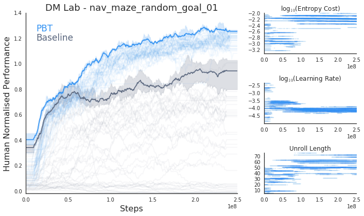
The high level results are summarised in Fig. 3. On all three domains – DeepMind Lab, Atari, and StarCraft II – PBT increases the final performance of the agents when trained for the same number of steps, compared to the very strong baseline of performing random search with the same number of workers.
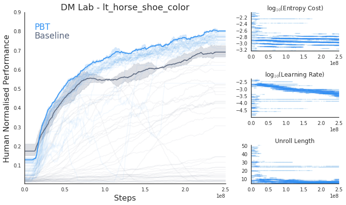
On DeepMind Lab, when UNREAL is trained using a population of 40 workers, using PBT increases the final performance of UNREAL from 93% to 106% human performance, when performance is averaged across all levels. This represents a significant improvement over an already extremely strong baseline, with some levels such as and showing large gains in performance due to PBT, as shown in Fig. 4. PBT seems to help in two main ways: first is that the hyperparameters are clearly being focused on the best part of the sampling range, and adapted over time. For example, on in Fig. 4 one can see the learning rate being annealed by PBT as training progresses, and on in Fig. 4 one can see the unroll length – the number of steps the agent (a recurrent neural network) is unrolled before performing N-step policy gradient and backpropagation through time – is gradually increased. This allows the agent to learn to utilise the recurrent neural network for memory, allowing it to obtain superhuman performance on which is a level which requires memorising the location of a goal in a maze, more details can be found in (jaderberg2016reinforcement). Secondly, since PBT is copying the weights of good performing agents during the exploitation phase, agents which are lucky in environment exploration are quickly propagated to more workers, meaning that all members of the population benefit from the exploration luck of the remainder of the population.
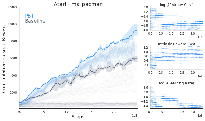
When we apply PBT to training FuN on 4 Atari levels, we similarly see a boost in final performance, with PBT increasing the average human normalised performance from 147% to 181%. On particular levels, such as PBT increases performance significantly from 6506 to 9001 (Fig. 4), which represents state-of-the-art for an agent receiving only pixels as input.
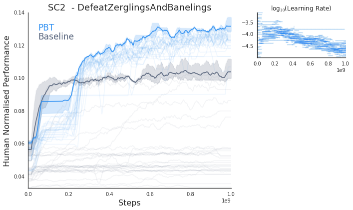
Finally on StarCraft II, we similarly see PBT improving A3C baselines from 36% huamn performance to 39% human performance when averaged over 6 levels, benefiting from automatic online learning rate adaptation and model selection such as shown in Fig. 4.
More detailed experimental results, and details about the specific experimental protocols can be found in Appendix A.2.
4.2 Machine Translation
As an example of applying PBT on a supervised learning problem, we look at training neural machine translation models. In this scenario, the task is to encode a source sequence of words in one language, and output a sequence in a different target language. We focus on English to German translation on the WMT 2014 English-to-German dataset, and use a state-of-the-art model, Transformer networks (vaswani2017attention), as the baseline model to apply PBT to. Crucially, we also use the highly optimised learning rate schedules and hyperparameter values for our baselines to compare to – these are the result of a huge amount of hand tuning and Bayesian optimisation.
4.2.1 PBT for Machine Translation
We use a population size of 32 workers, where each member of the population is a single GPU optimising a Transformer network for steps.
Hyperparameters
We allow PBT to optimise the learning rate, attention dropout, layer dropout, and ReLU dropout rates.
Step
Each step does a step of gradient descent with Adam (adam).
Eval
We evaluate the current model by computing the BLEU score on the WMT newstest2012 dataset. This allows us to optimise our population for BLEU score, which usually cannot be optimised for directly.
Ready
A member of the population is deemed ready to exploit and explore using the rest of the population every steps.
Exploit
We use the t-test selection exploitation method described in Sect. 4.1.1.
Explore
We explore hyperparameter space by the perturb strategy described in Sect. 4.1.1 with 1.2 and 0.8 perturbation factors.
4.2.2 Results
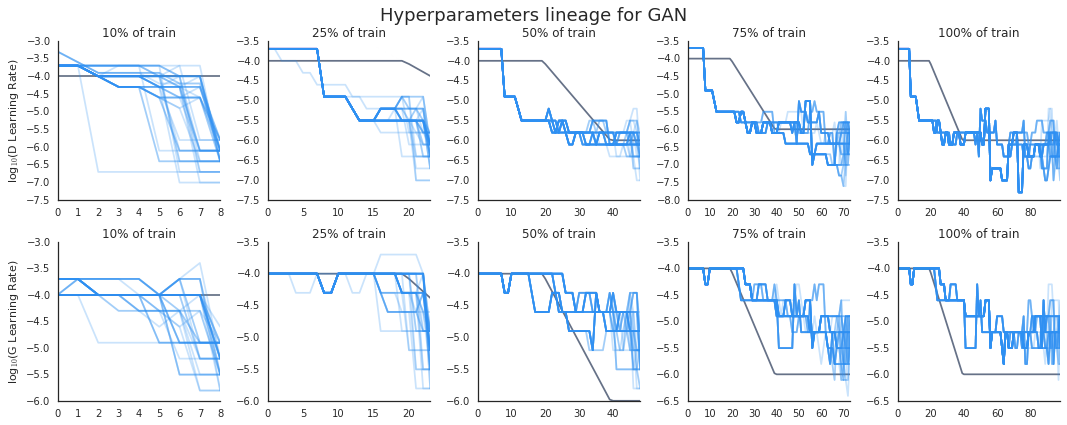
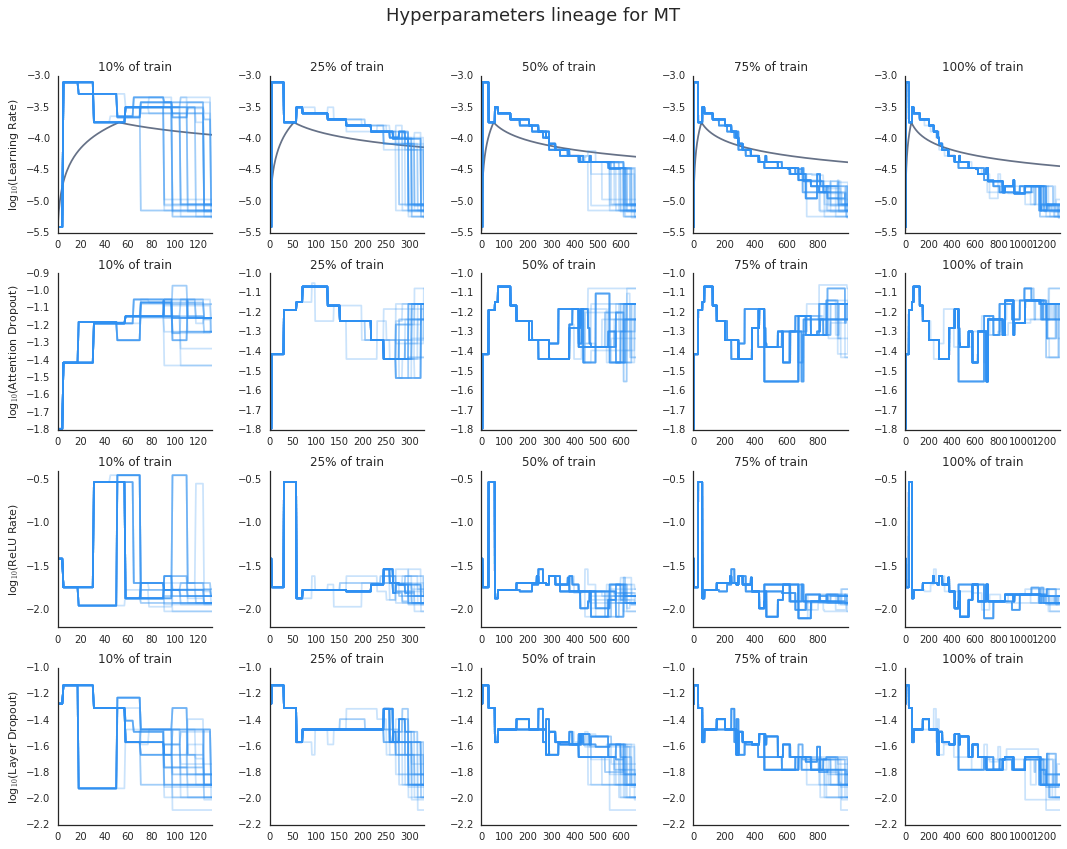
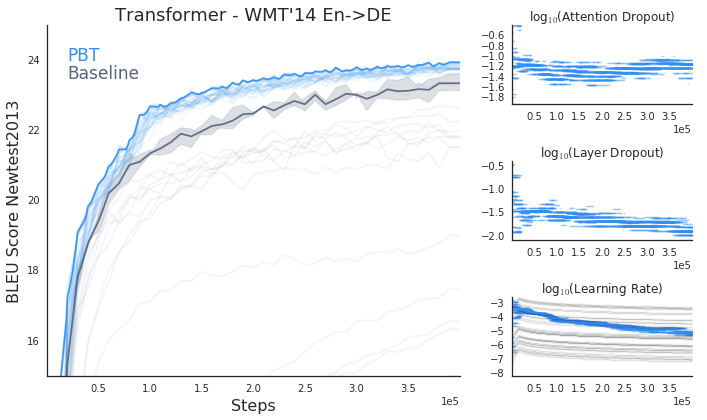
When we apply PBT to the training of Transformer networks, we find that PBT actually results in models which exceed the performance of this highly tuned baseline model: BLEU score on the validation set (newstest2012) is improved from 23.71 to 24.23, and on the test set of WMT 2014 English-to-German is improved from 22.30 to 22.65 using PBT (here we report results using the small Transformer network using a reduced batch size, so is not representative of state of the art). PBT is able to automatically discover adaptations of various dropout rates throughout training, and a learning rate schedule that remarkably resembles that of the hand tuned baseline: very initially the learning rate starts small before jumping by three orders of magnitude, followed by something resembling an exponential decay, as shown in the lineage plot of Fig. 7. We can also see from Fig. 4 that the PBT model trains much faster.
4.3 Generative Adversarial Networks
The Generative Adversarial Networks (GAN) (goodfellowgan) framework learns generative models via a training paradigm consisting of two competing modules – a generator and a discriminator (alternatively called a critic). The discriminator takes as input samples from the generator and the real data distribution, and is trained to predict whether inputs are real or generated. The generator typically maps samples from a simple noise distribution to a complex data distribution (e.g. images) with the objective of maximally fooling the discriminator into classifying or scoring its samples as real.
Like RL agent training, GAN training can be remarkably brittle and unstable in the face of suboptimal hyperparameter selection and even unlucky random initialisation, with generators often collapsing to a single mode or diverging entirely. Exacerbating these difficulties, the presence of two modules optimising competing objectives doubles the number of hyperparameters, often forcing researchers to choose the same hyperparameter values for both modules. Given the complex learning dynamics of GANs, this unnecessary coupling of hyperparameters between the two modules is unlikely to be the best choice.
Finally, the various metrics used by the community to evaluate the quality of samples produced by GAN generators are necessarily distinct from those used for the adversarial optimisation itself. We explore whether we can improve the performance of generators under these metrics by directly targeting them as the PBT meta-optimisation evaluation criteria.
4.3.1 PBT for GANs
We train a population of size 45 with each worker being trained for steps.
Hyperparameters
We allow PBT to optimise the discriminator’s learning rate and the generator’s learning rate separately.
Step
Each step consists of gradient descent updates of the discriminator followed by a single update of the generator using the Adam optimiser (adam). We train using the WGAN-GP (improvedwgan) objective where the discriminator estimates the Wasserstein distance between the real and generated data distributions, with the Lipschitz constraint enforced by regularising its input gradient to have a unit norm. See Appendix A.3 for additional details.
Eval
We evaluate the current model by a variant of the Inception score proposed by openaigan computed from the outputs of a pretrained CIFAR classifier (as used in mihaelaalphagan) rather than an ImageNet classifier, to avoid directly optimising the final performance metric. The CIFAR Inception scorer uses a much smaller network, making evaluation much faster.
Ready
A member of the population is deemed ready to exploit and explore using the rest of the population every steps.
Exploit
We consider two exploitation strategies. (a) Truncation selection as described in Sect. 4.1.1. (b) Binary tournament in which each member of the population randomly selects another member of the population, and copies its parameters if the other member’s score is better. Whenever one member of the population is copied to another, all parameters – the hyperparameters, weights of the generator, and weights of the discriminator – are copied.
Explore
We explore hyperparameter space by the perturb strategy described in Sect. 4.1.1, but with more aggressive perturbation factors of 2.0 or 0.5.
4.3.2 Results
We apply PBT to optimise the learning rates for a CIFAR-trained GAN discriminator and generator using architectures similar to those used DCGAN (dcgan). For both PBT and the baseline, the population size is , with learning rates initialised to for a total of initial hyperparameter settings, each replicated times with independent random weight initialisations. Additional architectural and hyperparameter details can be found in Appendix A.3. The baseline utilises an exponential learning rate decay schedule, which we found to work the best among a number of hand-designed annealing strategies, detailed in Appendix A.3.
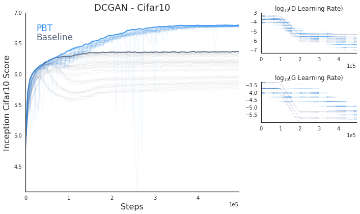
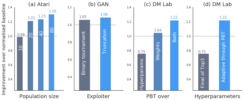
In Fig. 5 (b), we compare the truncation selection exploration strategy with a simpler variant, binary tournament. We find a slight advantage for truncation selection, and our remaining discussion focuses on results obtained by this strategy. Fig. 4 (bottom left) plots the CIFAR Inception scores and shows how the learning rates of the population change throughout the first half of training (both the learning curves and hyperparameters saturate and remain roughly constant in the latter half of training). We observe that PBT automatically learns to decay learning rates, though it does so dynamically, with irregular flattening and steepening, resulting in a learnt schedule that would not be matched by any typical exponential or linear decay protocol. Interestingly, the learned annealing schedule for the discriminator’s learning rate closely tracks that of the best performing baseline (shown in grey), while the generator’s schedule deviates from the baseline schedule substantially.
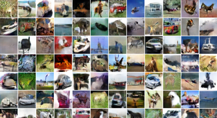
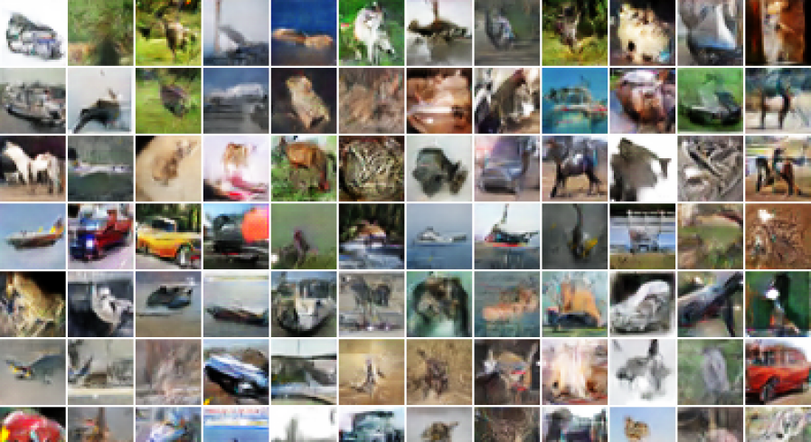
In Table 4 (Appendix A.3), we report standard ImageNet Inception scores as our main performance measure, but use CIFAR Inception score for model selection, as optimising ImageNet Inception score directly would potentially overfit our models to the test metric. CIFAR Inception score is used to select the best model after training is finished both for the baseline and for PBT. Our best-performing baseline achieves a CIFAR Inception score of , corresponding to an ImageNet Inception score of , similar to or better than Inception scores for DCGAN-like architectures reported in prior work (mihaelaalphagan; improvedwgan; lrgan). Using PBT, we strongly outperform this baseline, achieving a CIFAR Inception score of and corresponding ImageNet Inception score of . For reference, Table 4 (Appendix A.3) also reports the peak ImageNet Inception scores obtained by any population member at any point during training. Fig. 8 shows samples from the best generators with and without PBT.
4.4 Analysis
In this section we analyse and discuss the effects of some of the design choices in setting up PBT, as well as probing some aspects of why the method is so successful.
Population Size
In Fig. 5 (a) we demonstrate the effect of population size on the performance of PBT when training FuN on Atari. In general, we find that if the population size is too small (10 or below) we tend to encounter higher variance and can suffer from poorer results – this is to be expected as PBT is a greedy algorithm and so can get stuck in local optima if there is not sufficient population to maintain diversity and scope for exploration. However, these problems rapidly disappear as population size increases and we see improved results as the population size grows. In our experiments, we observe that a population size of between and is sufficient to see strong and consistent improvements; larger populations tend to fare even better, although we see diminishing returns for the cost of additional population members.
Exploitation Type
In Fig. 5 (b) we compare the effect of using different exploit functions – binary tournament and truncation selection. For GAN training, we find truncation selection to work better. Similar behaviour was seen in our preliminary experiments with FuN on Atari as well. Further work is required to fully understand the impact of different exploit mechanisms, however it appears that truncation selection is a robustly useful choice.
PBT Targets
In Fig. 5 (c) we show the effect of only applying PBT to subsets of parameters when training UNREAL on DM Lab. In particular, we contrast (i) only performing exploit-and-explore on hyperparameters (so model weights are not copied between workers during exploit); and (ii) only performing exploit-and-explore on model weights (so hyperparameters are not copied between workers or explored). Whilst there is some increase in performance simply from the selection and propagation of good model weights, our results clearly demonstrate that in this setting it is indeed the combination of optimising hyperparameters as well as model selection that lead to our best performance.
Hyperparameter Adaptivity
In Fig. 5 (d) we provide another demonstration that the benefits of PBT go beyond simply finding a single good fixed hyperparameter combination. Since PBT allows online adaptation of hyperparameters during training, we evaluate how important the adaptation is by comparing full PBT performance compared to using the set of hyperparameters that PBT found by the end of training. When training UNREAL on DeepMind Lab we find that the strength of PBT is in allowing the hyperparameters to be adaptive, not merely in finding a good prior on the space of hyperparameters
Lineages
Fig. 7 shows hyperparameter sequences for the final agents in the population for GAN and Machine Translation (MT) experiments. We have chosen these two examples as the community has developed very specific learning rate schedules for these models. In the GAN case, the typical schedule involves linearly annealed learning rates of both generator and discriminator in a synchronised way. As one can see, PBT discovered a similar scheme, however the discriminator annealing is much more severe, while the generator schedule is slightly less aggressive than the typical one.
As mentioned previously, the highly non-standard learning rate schedule used for machine translation has been to some extent replicated by PBT – but again it seems to be more aggressive than the hand crafted version. Quite interestingly, the dropout regime is also non-monotonic, and follows an even more complex path – it first increases by almost an order of magnitude, then drops back to the initial value, to slowly crawl back to an order of magnitude bigger value. These kind of schedules seem easy to discover by PBT, while at the same time are beyond the space of hyperparameter schedules considered by human experts.
Phylogenetic trees
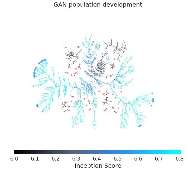
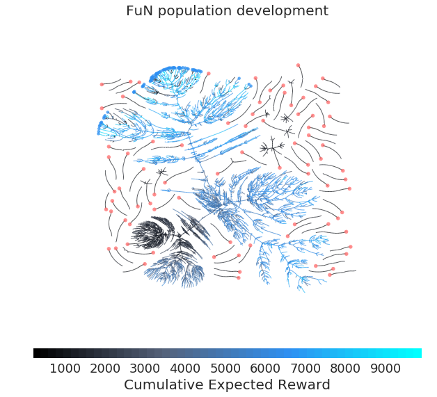
Figure 6 shows a phylogenetic forest for the population in the GAN and Atari experiments. A property made noticeable by such plots is that all final agents are descendants of the same, single initial agent. This is on one hand a consequence of the greedy nature of specific instance of PBT used, as exploit only uses a single other agent from the population. In such scenario, the number of original agents can only decrease over time, and so should finally converge to the situation observed. On the other hand one can notice that in both cases there are quite rich sub-populations which survived for a long time, showing that the PBT process considered multiple promising solutions before finally converging on a single winner – an exploratory capability most typical optimisers lack.
One can also note the following interesting qualitative differences between the two plots: in the GAN example, almost all members of the population enjoy an improvement in score relative to their parent; however, in the Atari experiment we note that even quite late in learning there can be exploration steps that result in a sharp drop in cumulative episode reward relative to the parent. This is perhaps indicative of some instability of neural network based RL on complex problems – an instability that PBT is well positioned to correct.
5 Conclusions
We have presented Population Based Training, which represents a practical way to augment the standard training of neural network models. We have shown consistent improvements in accuracy, training time and stability across a wide range of domains by being able to optimise over weights and hyperparameters jointly. It is important to note that contrary to conventional hyperparameter optimisation techniques, PBT discovers an adaptive schedule rather than a fixed set of hyperparameters. We already observed significant improvements on a wide range of challenging problems including state of the art models on deep reinforcement learning and hierarchical reinforcement learning, machine translation, and GANs. While there are many improvements and extensions to be explored going forward, we believe that the ability of PBT to enhance the optimisation process of new, unfamiliar models, to adapt to non-stationary learning problems, and to incorporate the optimisation of indirect performance metrics and auxiliary tasks, results in a powerful platform to propel future research.
Acknowledgments
We would like to thank Yaroslav Ganin, Mihaela Rosca, John Agapiou, Sasha Vehznevets, Vlad Firoiu, and the wider DeepMind team for many insightful discussions, ideas, and support.
References
- Agarwal et al. (2011) Alekh Agarwal, John C Duchi, Peter L Bartlett, and Clement Levrard. Oracle inequalities for computationally budgeted model selection. In Proceedings of the 24th Annual Conference on Learning Theory, pp. 69–86, 2011.
- Bäck (1998) Thomas Bäck. An overview of parameter control methods by self-adaptation in evolutionary algorithms. Fundamenta Informaticae, 35(1-4):51–66, 1998.
- Beattie et al. (2016) Charles Beattie, Joel Z Leibo, Denis Teplyashin, Tom Ward, Marcus Wainwright, Heinrich Küttler, Andrew Lefrancq, Simon Green, Víctor Valdés, Amir Sadik, et al. Deepmind lab. arXiv preprint arXiv:1612.03801, 2016.
- Bellemare et al. (2013) Marc G Bellemare, Yavar Naddaf, Joel Veness, and Michael Bowling. The arcade learning environment: An evaluation platform for general agents. J. Artif. Intell. Res.(JAIR), 47:253–279, 2013.
- Bergstra & Bengio (2012) James Bergstra and Yoshua Bengio. Random search for hyper-parameter optimization. Journal of Machine Learning Research, 13(Feb):281–305, 2012.
- Bergstra et al. (2011) James S Bergstra, Rémi Bardenet, Yoshua Bengio, and Balázs Kégl. Algorithms for hyper-parameter optimization. In Advances in Neural Information Processing Systems, pp. 2546–2554, 2011.
- Castillo et al. (1999) PA Castillo, V Rivas, JJ Merelo, Jesús González, Alberto Prieto, and Gustavo Romero. G-prop-iii: Global optimization of multilayer perceptrons using an evolutionary algorithm. In Proceedings of the 1st Annual Conference on Genetic and Evolutionary Computation-Volume 1, pp. 942–942. Morgan Kaufmann Publishers Inc., 1999.
- Castillo et al. (2006) PA Castillo, MG Arenas, JG Castellano, JJ Merelo, A Prieto, V Rivas, and G Romero. Lamarckian evolution and the Baldwin effect in evolutionary neural networks. arXiv preprint cs/0603004, 2006.
- Clune et al. (2008) Jeff Clune, Dusan Misevic, Charles Ofria, Richard E Lenski, Santiago F Elena, and Rafael Sanjuán. Natural selection fails to optimize mutation rates for long-term adaptation on rugged fitness landscapes. PLoS Computational Biology, 4(9):e1000187, 2008.
- Domhan et al. (2015) Tobias Domhan, Jost Tobias Springenberg, and Frank Hutter. Speeding up automatic hyperparameter optimization of deep neural networks by extrapolation of learning curves. In IJCAI, pp. 3460–3468, 2015.
- Fernando et al. (2016) Chrisantha Fernando, Dylan Banarse, Malcolm Reynolds, Frederic Besse, David Pfau, Max Jaderberg, Marc Lanctot, and Daan Wierstra. Convolution by evolution: Differentiable pattern producing networks. In Proceedings of the 2016 on Genetic and Evolutionary Computation Conference, pp. 109–116. ACM, 2016.
- Gloger (2004) Bartlomiej Gloger. Self adaptive evolutionary algorithms, 2004.
- Golovin et al. (2017) Daniel Golovin, Benjamin Solnik, Subhodeep Moitra, Greg Kochanski, John Karro, and D Sculley. Google vizier: A service for black-box optimization. In Proceedings of the 23rd ACM SIGKDD International Conference on Knowledge Discovery and Data Mining, pp. 1487–1495. ACM, 2017.
- González et al. (2016) Javier González, Zhenwen Dai, Philipp Hennig, and Neil Lawrence. Batch Bayesian optimization via local penalization. In Artificial Intelligence and Statistics, pp. 648–657, 2016.
- Goodfellow et al. (2014) Ian Goodfellow, Jean Pouget-Abadie, Mehdi Mirza, Bing Xu, David Warde-Farley, Sherjil Ozair, Aaron Courville, and Yoshua Bengio. Generative adversarial nets. In Advances in Neural Information Processing Systems, pp. 2672–2680, 2014.
- Gulrajani et al. (2017) Ishaan Gulrajani, Faruk Ahmed, Martin Arjovsky, Vincent Dumoulin, and Aaron Courville. Improved training of Wasserstein GANs. In Advances in Neural Information Processing Systems, pp. 5763–5773, 2017.
- György & Kocsis (2011) András György and Levente Kocsis. Efficient multi-start strategies for local search algorithms. Journal of Artificial Intelligence Research, 41:407–444, 2011.
- Houck et al. (1997) Christopher R Houck, Jeffery A Joines, Michael G Kay, and James R Wilson. Empirical investigation of the benefits of partial Lamarckianism. Evolutionary Computation, 5(1):31–60, 1997.
- Husken et al. (2000) Michael Husken, Jens E Gayko, and Bernhard Sendhoff. Optimization for problem classes-neural networks that learn to learn. In Combinations of Evolutionary Computation and Neural Networks, 2000 IEEE Symposium on, pp. 98–109. IEEE, 2000.
- Hutter et al. (2011) Frank Hutter, Holger H Hoos, and Kevin Leyton-Brown. Sequential model-based optimization for general algorithm configuration. LION, 5:507–523, 2011.
- Igel et al. (2005) Christian Igel, Stefan Wiegand, and Frauke Friedrichs. Evolutionary optimization of neural systems: The use of strategy adaptation. Trends and Applications in Constructive Approximation, pp. 103–123, 2005.
- Jaderberg et al. (2016) Max Jaderberg, Volodymyr Mnih, Wojciech Marian Czarnecki, Tom Schaul, Joel Z Leibo, David Silver, and Koray Kavukcuoglu. Reinforcement learning with unsupervised auxiliary tasks. arXiv preprint arXiv:1611.05397, 2016.
- Kingma & Ba (2015) Diederik Kingma and Jimmy Ba. Adam: A method for stochastic optimization. In ICLR, 2015.
- Klein et al. (2016) Aaron Klein, Stefan Falkner, Simon Bartels, Philipp Hennig, and Frank Hutter. Fast Bayesian optimization of machine learning hyperparameters on large datasets. arXiv preprint arXiv:1605.07079, 2016.
- Ku & Mak (1997) Kim WC Ku and Man-Wai Mak. Exploring the effects of Lamarckian and Baldwinian learning in evolving recurrent neural networks. In Evolutionary Computation, 1997., IEEE International Conference on, pp. 617–621. IEEE, 1997.
- Li et al. (2016) Lisha Li, Kevin Jamieson, Giulia DeSalvo, Afshin Rostamizadeh, and Ameet Talwalkar. Hyperband: A novel bandit-based approach to hyperparameter optimization. arXiv preprint arXiv:1603.06560, 2016.
- Liu et al. (2017) Hanxiao Liu, Karen Simonyan, Oriol Vinyals, Chrisantha Fernando, and Koray Kavukcuoglu. Hierarchical representations for efficient architecture search. arXiv preprint arXiv:1711.00436, 2017.
- Loshchilov & Hutter (2016) Ilya Loshchilov and Frank Hutter. SGDR: stochastic gradient descent with warm restarts. arXiv preprint arXiv:1608.03983, 2016.
- Massé & Ollivier (2015) Pierre-Yves Massé and Yann Ollivier. Speed learning on the fly. arXiv preprint arXiv:1511.02540, 2015.
- Mnih et al. (2016) Volodymyr Mnih, Adria Puigdomenech Badia, Mehdi Mirza, Alex Graves, Timothy Lillicrap, Tim Harley, David Silver, and Koray Kavukcuoglu. Asynchronous methods for deep reinforcement learning. In International Conference on Machine Learning, pp. 1928–1937, 2016.
- Radford et al. (2016) Alec Radford, Luke Metz, and Soumith Chintala. Unsupervised representation learning with deep convolutional generative adversarial networks. In ICLR, 2016.
- Rasley et al. (2017) Jeff Rasley, Yuxiong He, Feng Yan, Olatunji Ruwase, and Rodrigo Fonseca. Hyperdrive: Exploring hyperparameters with POP scheduling. In Proceedings of the 18th International Middleware Conference, Middleware, volume 17, 2017.
- Real et al. (2017) Esteban Real, Sherry Moore, Andrew Selle, Saurabh Saxena, Yutaka Leon Suematsu, Quoc Le, and Alex Kurakin. Large-scale evolution of image classifiers. arXiv preprint arXiv:1703.01041, 2017.
- Rosca et al. (2017) Mihaela Rosca, Balaji Lakshminarayanan, David Warde-Farley, and Shakir Mohamed. Variational approaches for auto-encoding generative adversarial networks. arXiv preprint arXiv:1706.04987, 2017.
- Sabharwal et al. (2016) Ashish Sabharwal, Horst Samulowitz, and Gerald Tesauro. Selecting near-optimal learners via incremental data allocation. In AAAI, pp. 2007–2015, 2016.
- Salimans et al. (2016) Tim Salimans, Ian Goodfellow, Wojciech Zaremba, Vicki Cheung, Alec Radford, and Xi Chen. Improved techniques for training GANs. In Advances in Neural Information Processing Systems, pp. 2234–2242, 2016.
- Salustowicz & Schmidhuber (1997) Rafal Salustowicz and Jürgen Schmidhuber. Probabilistic incremental program evolution: Stochastic search through program space. In ECML, pp. 213–220, 1997.
- Shah & Ghahramani (2015) Amar Shah and Zoubin Ghahramani. Parallel predictive entropy search for batch global optimization of expensive objective functions. In Advances in Neural Information Processing Systems, pp. 3330–3338, 2015.
- Smith (2017) Leslie N Smith. Cyclical learning rates for training neural networks. In Applications of Computer Vision (WACV), 2017 IEEE Winter Conference on, pp. 464–472. IEEE, 2017.
- Snoek et al. (2012) Jasper Snoek, Hugo Larochelle, and Ryan P Adams. Practical Bayesian optimization of machine learning algorithms. In Advances in neural information processing systems, pp. 2951–2959, 2012.
- Snoek et al. (2015) Jasper Snoek, Oren Rippel, Kevin Swersky, Ryan Kiros, Nadathur Satish, Narayanan Sundaram, Mostofa Patwary, Mr Prabhat, and Ryan Adams. Scalable Bayesian optimization using deep neural networks. In International Conference on Machine Learning, pp. 2171–2180, 2015.
- Spears (1995) William M. Spears. Adapting crossover in evolutionary algorithms. In Proceedings of the Fourth Annual Conference on Evolutionary Programming, pp. 367–384. MIT Press, 1995.
- Springenberg et al. (2016) Jost Tobias Springenberg, Aaron Klein, Stefan Falkner, and Frank Hutter. Bayesian optimization with robust Bayesian neural networks. In Advances in Neural Information Processing Systems, pp. 4134–4142, 2016.
- Srinivas et al. (2009) Niranjan Srinivas, Andreas Krause, Sham M Kakade, and Matthias Seeger. Gaussian process optimization in the bandit setting: No regret and experimental design. arXiv preprint arXiv:0912.3995, 2009.
- Swersky et al. (2013) Kevin Swersky, Jasper Snoek, and Ryan P Adams. Multi-task Bayesian optimization. In Advances in neural information processing systems, pp. 2004–2012, 2013.
- Swersky et al. (2014) Kevin Swersky, Jasper Snoek, and Ryan Prescott Adams. Freeze-thaw Bayesian optimization. arXiv preprint arXiv:1406.3896, 2014.
- Tieleman & Hinton (2012) Tijmen Tieleman and Geoffrey Hinton. Lecture 6.5-rmsprop: Divide the gradient by a running average of its recent magnitude. COURSERA: Neural networks for machine learning, 4(2):26–31, 2012.
- Vaswani et al. (2017) Ashish Vaswani, Noam Shazeer, Niki Parmar, Jakob Uszkoreit, Llion Jones, Aidan N Gomez, Lukasz Kaiser, and Illia Polosukhin. Attention is all you need. arXiv preprint arXiv:1706.03762, 2017.
- Vezhnevets et al. (2017) Alexander Sasha Vezhnevets, Simon Osindero, Tom Schaul, Nicolas Heess, Max Jaderberg, David Silver, and Koray Kavukcuoglu. Feudal networks for hierarchical reinforcement learning. arXiv preprint arXiv:1703.01161, 2017.
- Vinyals et al. (2017) Oriol Vinyals, Timo Ewalds, Sergey Bartunov, Petko Georgiev, Alexander Sasha Vezhnevets, Michelle Yeo, Alireza Makhzani, Heinrich Küttler, John Agapiou, Julian Schrittwieser, et al. Starcraft II: A new challenge for reinforcement learning. arXiv preprint arXiv:1708.04782, 2017.
- Welch (1947) Bernard L Welch. The generalization of student’s’ problem when several different population variances are involved. Biometrika, 34(1/2):28–35, 1947.
- Wu & Frazier (2016) Jian Wu and Peter Frazier. The parallel knowledge gradient method for batch Bayesian optimization. In Advances in Neural Information Processing Systems, pp. 3126–3134, 2016.
- Xue et al. (2016) Bing Xue, Mengjie Zhang, Will N Browne, and Xin Yao. A survey on evolutionary computation approaches to feature selection. IEEE Transactions on Evolutionary Computation, 20(4):606–626, 2016.
- Yang et al. (2017) Jianwei Yang, Anitha Kanna, Dhruv Batra, and Devi Parikh. LR-GAN: Layered recursive generative adversarial networks for image generation. In ICLR, 2017.
- Young et al. (2015) Steven R Young, Derek C Rose, Thomas P Karnowski, Seung-Hwan Lim, and Robert M Patton. Optimizing deep learning hyper-parameters through an evolutionary algorithm. In Proceedings of the Workshop on Machine Learning in High-Performance Computing Environments, pp. 4. ACM, 2015.
- Zhang et al. (2011) Jun Zhang, Zhi-hui Zhan, Ying Lin, Ni Chen, Yue-jiao Gong, Jing-hui Zhong, Henry SH Chung, Yun Li, and Yu-hui Shi. Evolutionary computation meets machine learning: A survey. IEEE Computational Intelligence Magazine, 6(4):68–75, 2011.
Appendix A Population Based Training of Neural Networks Appendix
A.1 Practical implementations
In this section, we describe at a high level how one might concretely implement PBT on a commodity training platform. Relative to a standard setup in which multiple hyperparameter configurations are searched in parallel (e.g. grid/random search), a practitioner need only add the ability for population members to read and write to a shared data-store (e.g. a key-value store, or a simple file-system). Augmented with such a setup, there are two main types of interaction required:
(1) Members of the population interact with this data-store to update their current performance and can also use it to query the recent performance of other population members.
(2) Population members periodically checkpoint themselves, and when they do so they write their performance to the shared data-store. In the exploit-and-explore process, another member of the population may elect to restore its weights from the checkpoint of another population member (i.e. exploiting), and would then modify the restored hyperparameters (i.e. exploring) before continuing to train.
As a final comment, although we present and recommend PBT as an asynchronous parallel algorithm, it could also be executed semi-serially or with partial synchrony. Although it would obviously result in longer training times than running fully asynchronously in parallel, one would still gain the performance-per-total-compute benefits of PBT relative to random-search. This execution mode may be attractive to researchers who wish to take advantage of commodity compute platforms at cheaper, but less reliable, preemptible/spot tiers. As an example of an approach with partial synchrony, one could imagine the following procedure: each member of the population is advanced in parallel (but without synchrony) for a fixed number of steps; once all (or some large fraction) of the population has advanced, one would call the exploit-and-explore procedure; and then repeat. This partial locking would be forgiving of different population members running at widely varying speeds due to preemption events, etc.
A.2 Detailed Results: RL
FuN - Atari
Table 1 shows the breakdown of results per game for FuN on the Atari domain, with and without PBT for different population sizes. The initial hyperparameter ranges for the population in both the FuN and PBT-FuN settings were the same as those used for the corresponding games in the original Feudal Networks paper (vezhnevets2017feudal), with the exception of intrinsic-reward cost (which was sampled in the range , rather than – since we have found that very low intrinsic reward cost weights are rarely effective). We used fixed discounts of in the worker and in the manager since, for the games selected, these were shown in the original FuN paper to give good performance. The subset of games were themselves chosen as ones for which the hierarchical abstractions provided by FuN give particularly strong performance improvements over a flat A3C agent baseline. In these experiments, we used Truncation as the exploitation mechanism, and Perturb as the exploration mechanism. Training was performed for agent-environmnent interactions, corresponding to total environment steps (due to use of action-repeat of ). Each experiment condition was repeated times, and the numbers in the table reflect the mean-across-replicas of the single best performing population member at the end of the training run.
| Game | Pop 10 | Pop 20 | Pop 40 | Pop 80 | ||||
|---|---|---|---|---|---|---|---|---|
| FuN | PBT-FuN | FuN | PBT-FuN | FuN | PBT-FuN | FuN | PBT-FuN | |
| amidar | 1742 174 | 1511 400 | 1645 158 | 2454 160 | 1947 80 | 2752 81 | 2055 113 | 3018 269 |
| gravitar | 3970 145 | 4110 225 | 3884 362 | 4202 113 | 4018 180 | 4481 540 | 4279 161 | 5386 306 |
| ms-pacman | 5635 656 | 5509 589 | 5280 349 | 5714 347 | 6177 402 | 8124 392 | 6506 354 | 9001 711 |
| enduro | 1838 37 | 1958 81 | 1881 63 | 2213 6 | 2079 9 | 2228 77 | 2166 34 | 2292 16 |
UNREAL - DM Lab
Table 2 shows the breakdown on results per level for UNREAL and PBT-UNREAL on the DM Lab domain. The following three hyperparameters were randomly sampled for both methods and subsequently perturbed in the case of PBT-UNREAL: the learning rate was sampled in the log-uniform range [0.00001, 0.005], the entropy cost was sampled in the log-uniform range [0.0005, 0.01], and the unroll length was sampled uniformly between 5 and 50 steps. Other experimental details were replicated from jaderberg2016reinforcement, except for pixel control weight which was set to 0.1.
| Game | Pop 40 | Pop 20 | ||||
|---|---|---|---|---|---|---|
| UNREAL | PBT-UNREAL | UNREAL | PBT-Hypers-UNREAL | PBT-Weights-UNREAL | PBT-UNREAL | |
| emstm_non_match | 66.0 | 66.0 | 42.6 | 14.5 | 56.0 | 53.2 |
| emstm_watermaze | 39.0 | 36.7 | 27.9 | 33.2 | 34.6 | 36.8 |
| lt_horse_shoe_color | 75.4 | 90.2 | 77.4 | 44.2 | 56.3 | 87.5 |
| nav_maze_random_goal_01 | 114.2 | 149.4 | 82.2 | 81.5 | 74.2 | 96.1 |
| lt_hallway_slope | 90.5 | 109.7 | ||||
| nav_maze_all_random_01 | 59.6 | 78.1 | ||||
| nav_maze_all_random_02 | 62.0 | 92.4 | ||||
| nav_maze_all_random_03 | 92.7 | 115.3 | ||||
| nav_maze_random_goal_02 | 145.4 | 173.3 | ||||
| nav_maze_random_goal_03 | 127.3 | 153.5 | ||||
| nav_maze_static_01 | 131.5 | 133.5 | ||||
| nav_maze_static_02 | 194.5 | 220.2 | ||||
| nav_maze_static_03 | 588.9 | 594.8 | ||||
| seekavoid_arena_01 | 42.5 | 42.3 | ||||
| stairway_to_melon_01 | 189.7 | 192.4 | ||||
A3C - StarCraft II
Table 2 shows the breakdown on results per level for UNREAL on the DM Lab domain, with and without PBT for different population sizes. We take the baseline setup of vinyals2017starcraft with feed-forward network agents, and sample the learning rate from the log-uniform range [0, 0.001].
| Game | Pop 30 | |
|---|---|---|
| A3C | PBT-A3C | |
| CollectMineralShards | 93.7 | 100.5 |
| FindAndDefeatZerglings | 46.0 | 49.9 |
| DefeatRoaches | 121.8 | 131.5 |
| DefeatZerglingsAndBanelings | 94.6 | 124.7 |
| CollectMineralsAndGas | 3345.8 | 3345.3 |
| BuildMarines | 0.17 | 0.37 |
A.3 Detailed Results: GAN
This section provides additional details of and results from our GAN experiments introduced in Sect. 4.3. Fig. 8 shows samples generated by the best performing generators with and without PBT. In Table 4, we report GAN Inception scores with and without PBT.
Baseline GAN
PBT-GAN
Architecture and hyperparameters
The architecture of the discriminator and the generator are similar to those proposed in DCGAN (dcgan), but with convolutions (rather than ), and a smaller generator with half the number of feature maps in each layer. Batch normalisation is used in the generator, but not in the discriminator, as in improvedwgan. Optimisation is performed using the Adam optimiser (adam), with , , and . The batch size is 128.
| GAN | PBT-GAN (TS) | PBT-GAN (BT) | |
|---|---|---|---|
| CIFAR Inception | 6.380.03 | 6.800.01 | 6.770.02 |
| ImageNet Inception (by CIFAR) | 6.450.05 | 6.890.04 | 6.740.05 |
| ImageNet Inception (peak) | 6.480.05 | 7.020.07 | 6.810.04 |
Baseline selection
To establish a strong and directly comparable baseline for GAN PBT, we extensively searched over and chose the best by CIFAR Inception score among many learning rate annealing strategies used in the literature. For each strategy, we trained for a total of steps, where learning rates were fixed to their initial settings for the first steps, then for the latter steps either (a) exponentially decayed to times the initial setting, or (b) linearly decayed to , searching over . (Searching over the number of steps is essential due to the instability of GAN training: performance often degrades with additional training.) In each training run to evaluate a given combination of annealing strategy and choice of training steps , we used the same number of independent workers () and initialised the learning rates to the same values used in PBT. The best annealing strategy we found using this procedure was exponential decay with steps. For the final baseline, we then extended this strategy to train for the same number of steps as used in PBT () by continuing training for the remaining steps with constant learning rates fixed to their final values after exponential decay.
A.4 Detailed Results: Machine Translation
We used the open-sourced implementation of the Transformer framework111https://github.com/tensorflow/tensor2tensor with the provided transformer_base_single_gpu architecture settings. This model has the same number of parameters as the base configuration that runs on 8 GPUs (), but sees, in each training step, of the number of tokens ( vs. ) as it uses a smaller batch size. For both evolution and the random-search baseline, we searched over learning rate, and dropout values applied to the attention softmax activations, the outputs of the ReLU units in the feed-forward modules, and the output of each layer. We left other hyperparameters unchanged and made no other changes to the implementation. For evaluation, we computed BLEU score based on auto-regressive decoding with beam-search of width 4. We used newstest2012 and newstest2013 respectively as the evaluation set used by PBT, and as the test set for monitoring. At the end of training, we report tokenized BLEU score on newstest2014 as computed by multi-bleu.pl script222https://github.com/moses-smt/mosesdecoder/blob/master/scripts/generic/multi-bleu.perl. We also evaluated the original hyperparameter configuration trained for the same number of steps and obtained the BLEU score of , which is lower than both our baselines and PBT results.